Double-Regulated Active Cruise Control for a Car Model with Nonlinear Powertrain Design

Abstract

The need for autonomous vehicles has started rising rapidly. Many autonomous technologies, such as Cruise Control, the self-parking system, and the emergency braking system, are implemented in contemporary cars. These systems do not make the car fully autonomous; however, they allow people to get used to the idea of self-driving cars. Due to a surge of interest in autonomous systems, the development of these technologies has begun. This paper presents a model of Adaptive Cruise Control with a control system, which consists of two PID regulators. Using two PID regulators provides the possibility of more advanced regulation characteristics than using the classical one-PID regulation system. One of them regulates the powertrain model, the other the braking system model. The simulations are carried out using a vehicle dynamic system, whose thrust is determined by a real engine maximum torque curve that is approximated by combinations of polynomial functions. Due to the non-linearity, caused by the motor’s curve and the use of two regulators, the PID tuning algorithm has been created. The algorithm provides satisfying results, followed by a marginal difference between the requested safe distance and actual distance value. The Active Cruise Control system has been tested using normalized driving cycles, which simulate the real behaviour of a car. The simulation results prove double-PID-regulated ACC’s accuracy and speed of response in different states of motion.

1. Introduction

The automotive industry [1,2,3,4] is currently striving for the introduction and production of autonomous vehicles for general use. The interest in vehicle automation is increasing, which is indicated by the large number of publications in that field [5,6,7,8,9]. Such vehicles must be equipped with intelligent systems that perform proper operations without the involvement of the driver, while ensuring comfort and safety while driving. The currently available vehicles use a wide variety of advanced systems that will be used as fundamental systems of future autonomous vehicles. Example of such systems are as follows: Lane Departure Warning, Blind Spot Detection, Road Sign Recognition, Adaptive Cruise Control, and Automatic Emergency Braking with an object recognition [10,11,12,13]. Nowadays, mathematical and simulation models of autonomous systems are commonly used at design stage. This approach allows one to verify the correctness of operation. Moreover, it provides a proper and accurate diagnosis of the facility without the need to build expensive prototype systems. Active Cruise Control is a system that can be described as an autonomous unit [13]. Its purpose is to adjust the following vehicle’s speed in order to maintain a safe distance [12] from the vehicle ahead [10,13,14,15]. The information about the distance between vehicles is obtained by sensors such a radars, lidars, or ultrasonic sensors [16,17,18]. Information that contains a measured distance is sent to the control system, whose function is to regulate the work of actuators responsible for accelerating or braking the vehicle. This kind of system allows one to relieve the driver, especially when driving in traffic jams and on a highway [13,14,19]. Therefore, the correct and reliable operation of the entire system determines driving safety and reduces the risk of road collision [13,14]. Simulation models of Adaptive Cruise Control used in vehicles are very popular in the scientific literature. This is due to the fact that the ACC system requires a control system, which necessitates research about many possibilities in the field of automation. According to the literature, the most popular approach is an ACC system that contains a single PI [20,21], PID [22], or LQR [20] regulator. These solutions allow one to build a simple model in terms of computation, which can be the basis for further development. More advanced Active Cruise Control systems include the Predictive Control Model [21,23,24,25,26,27] and Neural Network [27,28,29]. Vehicles models are built mainly as dynamic objects [21,22,25,27,30,31]. Furthermore, ACC modeling allows one to study the impact of this system on other systems in which the vehicle is equipped. In the literature, there are examples of analyses of electricity management [32] in electric and hybrid vehicles running with Active Cruise Control, as well as analyses of fuel consumption in vehicles with internal combustion engines [20,25,26]. ACC is also modelled in cooperation with other systems whose task is to relieve the driver, such as the stop and go system [22]. Other interesting examples are, firstly, the column of the vehicles equipped with the ACC system following one leading vehicle [33], and secondly, the ACC system with the possibility of switching to the Cruise Control system [14].

The utilization of the double PID system is a topic of current investigation. There are applications of double loop control systems in active suspension systems [34]. This shows that the double PID system can increase the effectiveness of the control system. It seems to be an interesting solution to the problem of the application of the double PID system in the case of ACC and allows one to investigate the dynamics of such a solution.

The purpose of this research is to present a simulation model of Adaptive Cruise Control, whose control system is equipped with two regulators. One regulator will be responsible for the operation of the powertrain model and the other for the operation of the braking system model. This solution makes it possible to simulate these two systems in such a way that they do not work at the same time and allow one to take into account different operating characteristics. Regulators of this type are widely used in the automotive field, for example, in the semi-active suspension control system [35]. The usage of PID-type regulators results from the fact that they use output and input signals to regulate the systems without interfering with the internal parameters of the object [7,36]. In order to select regulators correctly, it has been decided to create a computing environment in Python 3.7. It was decided to use the DynPy library and the Jupyter tool. The DynPy library is an object-oriented tool that provides a modular approach to physical phenomena. DynPy is developed or maintained by the Authors of the article [37,38]. The Jupyter notebook is a popular runtime environment for various scripts or macros written in scripting programming languages such as Python or R. It can support designers in the process of preliminary parameter selection and makes a valuable contribution to similar solutions.

This paper focuses on the analysis of the ACC mathematical model controllers based on two PID separate regulators. For this purpose, the following steps are taken:

-

The usage of a mathematical dynamic model of vehicle for the initial investigation of control parameters (enabling the control of such systems in a more efficient way),

-

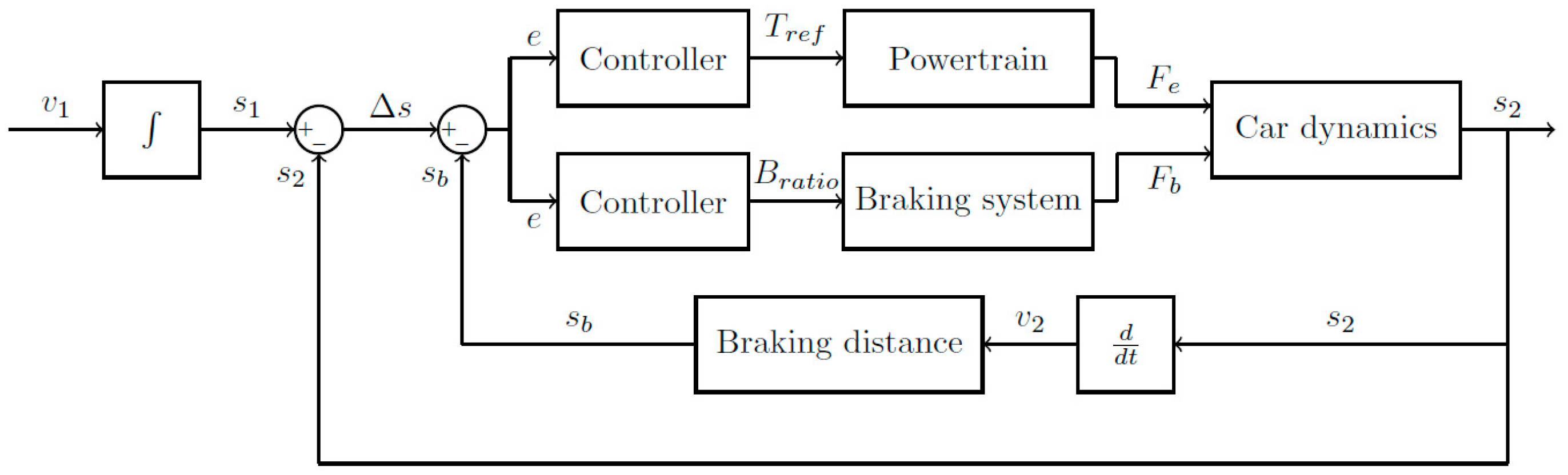
The application of the system of the double PID controller for drive and braking systems,

-

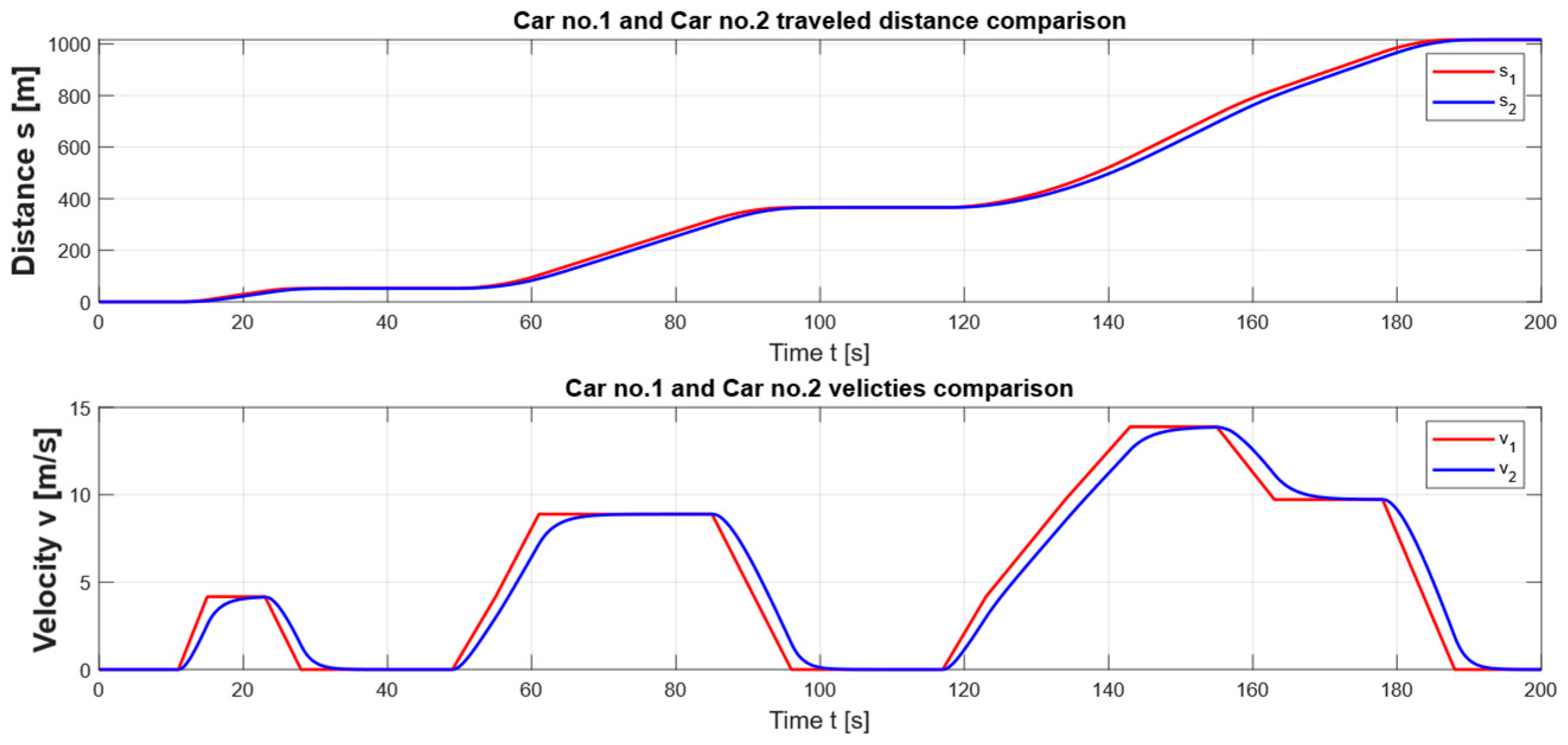
Numerical simulations are used for the theoretical validation of the proposed solution.

This paper discusses the novelty of using two of them separately. Other cases are not investigated because of preliminary character of this study. It aims to show the efficiency of proposed solution.

2. Simulation Models as a Way of Active Cruise Control Development

Simulation models are fundamental to autonomous system research thanks to simulation environment advancement. Designing such systems does not require one to build a prototype model at the beginning of the process, which means this approach is economically beneficial. Moreover, simulation environments are commonly used in various companies and at universities, so future employees will no longer need a sped-up design process.

Active Cruise Control systems utilize various controllers such as PID or PD controllers, LQR controllers, or regulation systems based on the fuzzy logic. The most common approach is to use the model with the PID control system due to its simplicity. This is because the controller does not need a lot of computing resources. The lack of difficult computing provides such control system diversity. This means the controller can be used in kinematic and dynamic systems with multiple degrees of freedom.

There are two main strategies of ACC design. The first of them is a single-degree-of-freedom (SDOF) dynamic model, which utilizes a signal from sensors to compute the proper engine force. This force is used to accelerate a vehicle and control the velocity to keep a safe distance between the leading car and the following car. The ACC system also requires a braking system control to decrease emergency velocity. The second approach is a multiple-degrees-of-freedom (MDOF) dynamic system, which works similar to the SDOF model but also controls the steering system to keep a vehicle in a proper position between the lane lines. It also adjusts the velocity in the corners.

The proposed ACC simulation model (Figure 1) is a SDOF dynamic system that adjusts a velocity by controlling a distance between the leading car and the following car.

The velocity is controlled by the force that the model of the engine produces. The correct thrust value is calculated with the usage of engine maximum torque curve.

A block diagram of the control system is shown in the Figure 2.

The ACC model has been designed in MATLAB Simulink 2024. That environment allows one to prepare mathematical models of dynamic objects, and it is equipped with the Control System Toolbox, which includes a PID controller. The authors decided to use this software according to the extent of the results’ correctness. The obtained results will be a base for the further development of specialized software in a Python 3.7 environment.

3. Modeling Methodology

The ACC system has been developed for the analytical vehicle model. The physics of car model movement has been determined by formulas that represents particular resistance forces. The force needed to initiate vehicle movement is generated by a model of a powertrain that consists of a gearbox, gearshift, engine, and torque converter. The parameters of mentioned parts have been based on the model of a 2017 Honda Civic 5d 1.5 VTEC Turbo Sport. To reduce velocity, the braking system has been implemented. The braking system determines a braking force accordingly to a current state of a motion. It adjusts to decelerate a vehicle in situations where the inertia of the engine rotational elements is insufficient to reduce the speed and keep a safe distance. The power train and braking system are provided with an individual control system. The sequence of an activation for each element is determined by the prepared logic layout. The correct activation sequence is based on a difference between the cars relative distance and the calculated safe distance. To perform a simulation, the authors assumed that the movement of a leading car will be represented by the NEDC driving cycle. The selection of a driving cycle has been determined by its simple shape and the appearance of an urban cycle and extra-urban cycle. These two sections allow one to simulate the ability of controlling the full range of a car duty cycle. According to the single-degree-of-freedom vehicle model, the authors assumed that the vehicle is moving in a straight line on a flat asphalt road. The choice of a simulated environment is due to the necessity of obtaining a benchmark result for the software development in Python 3.7 and the fact that the variable surface friction coefficient and road slope can be simulated as additional forces with harmonic disturbance and tested in further research. During simulations, the vehicle has been exposed to resistance forces such as friction, drag, and inertia resistance. Utilizing the assumption that the force generated by the engine is equal to or greater than the sum of resistance forces in the system, it is possible to create the equation of motion presented in Equation (1).

$$m_{red}\ddot{x}=F_e-m·g·f_0·\kappa ·{\dot{x}}^2-{\displaystyle \frac{1}{2}}·A·c_x·\rho ·{\dot{x}}^2-F_b$$

(1)

where $\ddot{x}$—the acceleration of the vehicle ${\displaystyle \frac{\mathrm{m}}{{\mathrm{s}}^2}}$, $\dot{x}$—the velocity of the vehicle ${\displaystyle \frac{\mathrm{m}}{\mathrm{s}}}$, $m_{red}$—the vehicle’s reduced mass $m_{red}=1831.6 \mathrm{kg}$, $F_e$—the thrust $\mathrm{N}$, $m$—the total mass of the vehicle $m=1760.0 \mathrm{kg}$, $g$—the acceleration of the gravity $g=9.81 {\displaystyle \frac{\mathrm{m}}{{\mathrm{s}}^2}}$, $f_0$—the friction coefficient $f_0=0.01$, $\kappa$—the proportional factor $\kappa ={10}^{-5} {\displaystyle \frac{\mathrm{s}}{\mathrm{m}}}$, $A$—the frontal area of the vehicle ${A=2.14 \mathrm{m}}^2$, $c_x$—the drag coefficient $c_x=0.28$, $\rho$—the air density $\rho =1.2 {\displaystyle \frac{\mathrm{k}\mathrm{g}}{{\mathrm{m}}^3}}$, and $F_b$—the braking force $\mathrm{N}$.

The block scheme of a simulation model is shown in Figure 3. It represents a functional principle of the system. Each part of the system has been represented by a block that contains the functions required to perform its function.

At the entry to the system, the velocity of the leading car is given (the NEDC cycle). The velocity is used to obtain the currently travelled distance and calculate the relative distance between the leading car and the following car. The relative distance is used in error calculation. To calculate the error, the following formulas have been used [39]:

$$s_b=v_2·\left(t_r+t_o+{\displaystyle \frac{t_n}{2}}\right)+{\displaystyle \frac{v_2^2}{2a_b}}$$

(2)

$$e=\left(s_1-s_2\right)-s_b$$

(3)

where $s_b$—the safe distance $\mathrm{m}$, $v_2$—the velocity of the following car ${\displaystyle \frac{\mathrm{m}}{\mathrm{s}}}$, $t_r$—the driver’s psychomotor reaction time $t_r=1.12 \mathrm{s}$, $t_o$—the brake system delay time $t_o=0.05 \mathrm{s}$, $t_n$—the braking force increase time $t_n=0.17 \mathrm{s}$, and $a_b$—the braking deceleration $a_b=10.0 {\displaystyle \frac{\mathrm{m}}{{\mathrm{s}}^2}}$.

In the next stage, the system checks a sign for the error. The error sign determined which controller should be activated in current situation. The value of an error is a base for the reference torque and braking ratio. The calculated reference values apply to proper blocks that represent powertrain or braking systems, where the thrust and braking force are obtained. At the end of the cycle, the generated forces apply to the part of the simulation that represents the car dynamics. The car dynamics simulation block applies to the distance travelled by the following car and closes the loop.

The powertrain model has been presented in Figure 4. This scheme represents an ideological model of the powertrain system, which has been used in simulations.

The powertrain block consists of the following parts:

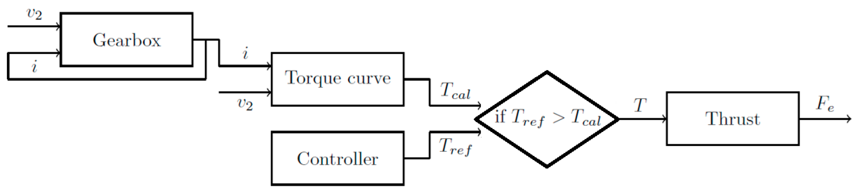
• The gearbox block, with which the gear and transmission are chosen. The gear choice is intent on simple logic functions. The main goal of this block is to increase the range of a torque curve;
• The torque curve block, which represents the implemented functions responsible for calculating the maximum available torque for the current rotational speed. Calculations are carried out with an use of approximated polynomial function that represents the real maximum torque curve of a simulated car;
• The controller, with which the reference value is obtained;
• The function block, which represents the functions liable for adjusting a proper throttle open angle. It is obtained with the use of a prepared logic layout;
• The thrust block, which represents a torque converter. This block consists of a function that calculates an engine force based on the current gear and the system’s dynamic variables.

Presented models (Figure 3 and Figure 4) are a mathematical background for further analyses due to control system development and numerical investigation.

4. Control System Development

The Designed Active Cruise Control system has been built with the use of two regulators. The regulator that is responsible for torque adjusting is a PD controller. The authors decided to abandon the Integral element due to the nature of it. The Integral element causes further incorrect regulation, which is unacceptable for that kind of system. The braking system is regulated by a P controller. This choice has been determined by the fact that braking depends on a temporary state of a motion, which does not require the anticipation of a further relative distance decrease.

A model of a controller is represented by the block scheme in Figure 5. It shows an idea of a control system implemented in the Active Cruise Control model.

The control system checks the sign with a conditional function. The output of a conditional function dictates the activation of a proper controller branch. The positive value of an error means that the PD controller has to calculate the initial reference torque value, and subsequently it is adjusted to the engine capabilities.

The braking regulation branch works similarly to the previously described one. The proportional regulator determines a braking ratio, which is a value from 0 to 100% of a maximum deceleration value. The saturation block keeps the deceleration at a realistic level to keep the simulation more valuable.

The controller settings have been obtained due to the stability test carried out on the system. In order to perform the preliminary selection of the controller parameters, the analytical environment (written in Python) was established. The settlement of the environment is determined by two elements: the notebook is to create and the dynamic system is to initiate. Dynamic systems are implemented in the modules or can be added to the calculation environment by the inheritance [38]. For the test equation, (1) has been linearized in neighbourhood of an operating point within a created script. The operating point is for a vehicle movement at a stable velocity equal to 50.0 km/h. The linearized equation of motion with substituted engine force is presented as Equation (4):

$$m_{\mathit{red}}\ddot{x}+f_{0}g{m}_{\mathit{red}}(\kappa \dot{x})+13Acₓ\rho \dot{x}-{\displaystyle \frac{169Acₓ\rho }{2}}-D(v_{\mathit{ref}}+\ddot{x})-P(t{v}_{\mathit{ref}}+\dot{x})+{\displaystyle \frac{0.021\eta i^3{i}_c^3\dot{x}-0.135\eta i^3{i}_c^3}{r_d^3}}-{\displaystyle \frac{0.638\eta i^2{i}_c^2\dot{x}}{r_d^2}}-{\displaystyle \frac{121.874\eta i{i}_c}{r_d}}=0$$

(4)

where $P$—the proportional element setting, $D$—the derivative element setting, $v_{ref}$—the reference velocity, $\eta$—the torque transmission efficiency $\eta =0.9$, $i$—the current gear transmission value $i_1=3.643$, $i_2=2.08, i_3=1.361, i_4=1.024, i_5=0.83, i_6=0.686, i_c$—the main gear transmission value $i_c=4.105$, $r_d$—the dynamic rolling radius of the wheel $r_d=0.312 \mathrm{m}$, and $t$—time s.

The linearized equation of motion is a first-order differential equation due to the lack of a position variable $x$. Thanks to that, it is possible to predict a simple solution in the following form:

$$\dot{x}=D{e}^{-{\displaystyle \frac{C}{M}}·t }$$

(5)

where $D$—the constant value, $C$—the sum of coefficients next to the velocity $\dot{x}$, and $M$—the sum of coefficients next to the acceleration $\ddot{x}$.

According to common knowledge, the $e^{-{\displaystyle \frac{C}{M}}·t }$ function approaches zero when the coefficient next to the variable $t$ is less than 0. This means that the particular situation ${\displaystyle \frac{C}{M}}$ has to be greater than 0. Utilizing that assumption, it is possible to create a relation between the P and D settings, which is presented in Equation (6):

$$P={10}^{-16}·({\displaystyle \frac{-2.08·{10}^{14}\eta i^3{i_c}^3+6.38·{10}^{15}\eta i^2{i_c}^2{r}_d}{{r_d}^3}}+{\displaystyle \frac{{10}^{15}{r_d}^3(-130A{c}_x\rho +D-10f_{0}g\kappa m_{red}+m_{red})}{{r_d}^3}})$$

(6)

The best way to obtain an equation was to assume a value greater than zero. In that research, the assumed convergence value was 0.1 and the derivative setting value was 10. Thanks to that, the proportional element setting value was equal to 226. Equation (5) presents the dynamic response of the system in the neighborhood of the operation point. The root of the characteristic polynomial of the system can be obtained directly. The real part of the root ensures a stable regulation process. This is caused by condition (6).

5. Simulation Analysis

The simulation has been carried out with an use of obtained regulator settings. The simulation time is equal to the NEDC cycle—1180.0 s, and the simulation step was set as 0.0001. The following figures illustrate the most representative values of the parameters.

Figure 6 presents the changes in the error (from Figure 5) in the full NEDC cycle. The chart is represented by error peaks that are rapidly eliminated. It shows the controller response capabilities. The extreme error values are 0.1638 m and −0.004 m in the urban cycle, and 0.4115 m and 0.008 m in the extra-urban cycle.

The powertrain and braking system parameters have been illustrated in Figure 7. A chart of an engine rotational speed has been used to check the correctness of the gearbox functionality. It contains characteristic peaks that are a representation of gear change moment. The gear change can be also seen in the engine and brakes forces plot. A change is a reason for the sudden force drop, which is the cause of transmission to the less effective part of the torque curve. The time series of the braking force and engine force shows that those two systems work independently and maintain process continuity, which confirms the proposed solution.

A comparison of the distances travelled by cars and their velocities is presented in Figure 8.

In Figure 8, the simulation time has been shortened to provide accurate results. The first subplot shows the influence of an adaptable safe distance assortment where the difference between cars positions increases due to the higher velocity. The tracking vehicle travels a shorter distance according to the safe distance. The second subplot of Figure 8 shows that the adaptable distance does not have negative effect at the velocity regulation, due to the lack of overshoot. The acceleration and braking are smooth and gentle, ensuring the comfort and safety of driver and passengers. These are the significant advantages of the proposed method, and they provide for the possibility of developing new control strategies.

6. Summary

Concluding the research, it is assumed that implemented Active Cruise Control can be utilized as a basis for further ACC system development as well as an acceptable model for the automotive industry. The presented graphs of the control system, powertrain, braking system, and vehicle kinematic parameters contain valuable results that confirm the correctness work of that system. The simplicity of the simulation parameters implementation allows one to substitute the simulated vehicle model with other conventional or hybrid vehicles [15] and obtain valuable results. The accomplished control system ensures a wide range of control capabilities that allow one to carry out simulations for the other vehicle variants with minor adjustments to the regulators’ settings.

The designed ACC model allows one to replace the utilized controllers with more advanced regulators. Additionally, the system is adapted to the implementation of the fuzzy logic control system and different autonomous systems. That way of development may involve the data source regarding the influence and reliability of ACC and different autonomous system combinations.

Another way of presented vehicle model development is the addition of different degrees of motion. This way of system enlargement may increase a variety of controllable parameters. The result would be velocity adjusting in variable conditions such as lane changing or passing at an intersection.

The Matlab Simulink such as 2020 version simulation environment is commonly assumed as a reasonable simulation software. Accordingly, the obtained results may be used to validate the outcome from the development simulation environment in Python. The purpose of having one’s own software development is diversity that may be obtained due to the more specialized environment.

The prospects for further the development of the presented solution are related to the comparison of results with other control methods. Such an approach will allow one to determine the advantages and disadvantages of the proposed solution, which was not in the scope of this work. The next step the authors are going to take is to compare this solution with other works related to different control systems. It is necessary to compare those systems to choose the best parameters as well as the setup for ACC systems. The further development of the presented solution is going to indicate the imperfections of this solution as well as the potential for its development and improvement.

References

1. Li, L.; Zhou, C.; Huang, J.; Liu, Z.; Xie, J.; Tan, Z. Car-following safety modeling risk assessment of autonomous vehicle in icy and snowy weather. Accid. Anal. Prev. 2025, 214, 107982. [Google Scholar] [CrossRef] [PubMed]
2. Channamallu, S.S.; Almaskati, D.; Kermanshachi, S.; Pamidimukkala, A. Autonmous vehicle safety: An advanced bagging classifier technique for crash injury prediction. Multimodal Transporation 2025, 4, 100189. [Google Scholar] [CrossRef]
3. Zhao, Y.; Zhu, Y.; Zhao, L.; Huang, J.; Zhi, Q. Behavioral decision-making and safety verification approaches for autonomous driving system in extreme scenarios. J. Syst. Softw. 2025, 226, 112385. [Google Scholar] [CrossRef]
4. Wang, X.; Qian, B.; Zhou, J.; Liu, W. An Autonomous Vehicle Behavior Decision Method Based on Deep Reinforcement Learning with Hybrid State Space and Driving Risk. Sensors 2025, 25, 774. [Google Scholar] [CrossRef]
5. Fagnant, D.J.; Kockelman, K. Preparing a nation for autonomous vehicles: Opportunities, barriers and policy recommendations. Transp. Res. Part A Policy Pract. 2015, 77, 167–181. [Google Scholar] [CrossRef]
6. Faisal, A.; Yigitcanlar, T.; Kamruzzaman, M.d.; Currie, G. Understanding autonomous vehicles: A systematic literature review on capability, impact, planning and policy. J. Transp. Land Use 2019, 12, 45–72. [Google Scholar] [CrossRef]
7. Johnson, M.A.; Moradi, M.H.; Crowe, J. PID Control: New Identification and Design Methods; Springer: New York, NY, USA, 2005. [Google Scholar]
8. Martínez-Díaz, M.; Soriguera, F. Autonomous vehicles: Theoretical and practical challenges. Transp. Res. Procedia 2018, 33, 275–282. [Google Scholar] [CrossRef]
9. Rojas-Rueda, D.; Nieuwenhuijsen, M.J.; Khreis, H.; Frumkin, H. Autonomous Vehicles and Public Health. Annu. Rev. Public Health 2020, 41, 329–345. [Google Scholar] [CrossRef]
10. Boruta, G.; Piętak, A. Mechatronika Samochodu: Układy Bezpieczeństwa Czynnego i Biernego; Wydawnictwo Uniwersytetu Warmińsko-Mazurskiego: Olsztyn, Poland, 2012. [Google Scholar]
11. Fischer-Wolfarth, J.; Meyer, G. Advanced Microsystems for Automotive Applications; Springer International Publishing: Cham, Switzerland, 2014. [Google Scholar]
12. Olejnik, K. Permissible distance—Safety system of vehicles in use. Open Eng. 2021, 11, 303–309. [Google Scholar] [CrossRef]
13. Rajamani, R. Vehicle Dynamics and Control; Springer: New York, NY, USA, 2006. [Google Scholar]
14. Shakouri, P.; Ordys, A. Nonlinear Model Predictive Control approach in design of Adaptive Cruise Control with automated switching to cruise control. Control Eng. Pract. 2014, 26, 160–177. [Google Scholar] [CrossRef]
15. Sun, X. Design of ACC Adaptive Cruise System Based on Ultrasonic Ranging and Internet of Vehicles. J. Phys. Conf. Ser. 2020, 1650, 022029. [Google Scholar] [CrossRef]
16. Baum, D.; Hamann, C.D.; Schubert, E. High Performance ACC System Based on Sensor Fusion with Distance Sensor, Image Processing Unit, and Navigation System. Veh. Syst. Dyn. 1997, 28, 327–338. [Google Scholar] [CrossRef]
17. Bian, N.; Liu, J.; Du, J.; Guo, S.; Yang, Y.; Chen, J.; Shi, T.; Yue, Z. The Development and Application of ACC System. In Proceedings of the 2014 Sixth International Conference on Measuring Technology and Mechatronics Automation, Zhangjiajie, China, 10–11 January 2014; pp. 692–695. [Google Scholar]
18. Pananurak, W.; Thanok, S.; Parnikchun, M. Adaptive cruise control for an intelligent vehicle. In Proceedings of the 2008 IEEE International Conference on Robotics and Biomimetics, Bangkok, Thailand, 22–25 February 2009; pp. 1794–1799. [Google Scholar]
19. Qing, X.; Hedrick, K.; Sengupta, R.; VanderWerf, J. Effects of vehicle-vehicle/roadside-vehicle communication on adaptive cruise controlled highway systems. In Proceedings of the IEEE 56th Vehicular Technology Conference, Vancouver, BC, Canada, 24–28 September 2002; pp. 1249–1253. [Google Scholar]
20. Park, C.; Lee, H. A Study of Adaptive Cruise Control System to Improve Fuel Efficiency. Int. J. Environ. Pollut. Remediat. 2017, 5, 15–19. [Google Scholar] [CrossRef]
21. Shakouri, P.; Ordys, A.; Laila, D.S.; Askari, M. Adaptive Cruise Control System: Comparing Gain-Scheduling PI and LQ Controllers. IFAC Proc. Vol. 2011, 44, 12964–12969. [Google Scholar] [CrossRef]
22. Sivaji, V.V.; Sailaja, D.M. Adaptive Cruise control systems for vehicle modeling using stop and go manoeuvres. Int. J. Eng. Res. Appl. 2013, 3, 2453–2456. [Google Scholar]
23. Guo, L.; Ge, P.; Sun, D.; Qiao, Y. Adaptive Cruise Control Based on Model Predictive Control with Constraints Softening. Appl. Sci. 2020, 10, 1635. [Google Scholar] [CrossRef]
24. Mao, J.; Yang, L.; Hu, Y.; Liu, K.; Du, J. Research on Vehicle Adaptive Cruise Control Method Based on Fuzzy Model Predictive Control. Machines 2021, 9, 160. [Google Scholar] [CrossRef]
25. Nie, Z.; Farzaneh, H. Adaptive Cruise Control for Eco-Driving Based on Model Predictive Control Algorithm. Appl. Sci. 2020, 10, 5271. [Google Scholar] [CrossRef]
26. Ruina, D.; He, C.; Qiang, Z.; Keqiang, L.; Yusheng, L. ACC of electric vehicles with coordination control of fuel economy and tracking safety. In Proceedings of the 2012 IEEE Intelligent Vehicles Symposium, Madrid, Spain, 3–7 June 2012; pp. 240–245. [Google Scholar]
27. Wang, M.; Yu, H.; Dong, G.; Huang, M. Dual-Mode Adaptive Cruise Control Strategy Based on Model Predictive Control and Neural Network for Pure Electric Vehicles. In Proceedings of the 2019 5th International Conference on Transportation Information and Safety, Liverpool, UK, 14–17 July 2019; pp. 1220–1225. [Google Scholar]
28. Mu, H.; Li, L.; Mei, M.; Zhao, Y. A hierarchical Control Scheme for Adaptive Cruise Control System Based on Model Predictive Control. Actuators 2023, 12, 249. [Google Scholar] [CrossRef]
29. Yang, Z.; Wang, Z.; Yan, M. An Optimization Design of Adaptive Cruise Control System Based on MPC and ADRC. Actuators 2021, 10, 110. [Google Scholar] [CrossRef]
30. Mohd, T.A.T.; Hassan, M.K.; Aziz, W.A. Mathematical modeling and simulation of an electric vehicle. J. Mech. Eng. Sci. 2015, 30, 1312–1321. [Google Scholar] [CrossRef]
31. Szost, K. Simulation model of a vehicle with an internal combustion engine and automatic gearbox. Przemysł Chem. 2024, 103, 1548–1552. [Google Scholar]
32. Khayyam, H.; Nahavandi, S.; Davis, S. Adaptive cruise control look-ahead system for energy management of vehicles. Expert Syst. Appl. 2012, 39, 3874–3885. [Google Scholar] [CrossRef]
33. Luu, D.L.; Lupu, C.; Van Nguyen, T. Design and Simulation Implementation for Adaptive Cruise Control Systems of Vehicles. In Proceedings of the 2019 22nd International Conference on Control Systems and Computer Science, Bucharest, Romania, 28–30 May 2019; pp. 1–6. [Google Scholar]
34. Tan, D.; Lu, C.; Zhang, X. Dual-loop PID control with PSO algorithm for the active suspension of the electric vehicle driven by in-wheel motor. J. Vibroengineering 2016, 18, 3915–3929. [Google Scholar] [CrossRef]
35. Narwade, P.; Deshmukh, R.; Nagarkar, M.; Bankar, M. Modeling and Simulation of a Semi-active Vehicle Suspension system using PID Controller. IOP Conf. Ser. Mater. Sci. Eng. 2020, 1004, 12003. [Google Scholar] [CrossRef]
36. Ang, K.H.; Chong, G.C.Y.; Li, Y. PID control system analysis, design, and technology. IEEE Trans. Control Syst. Technol. 2005, 13, 559–576. [Google Scholar]
37. Sierociński, D.; Chiliński, B.; Gawiński, F.; Radomski, A.; Przybyłowicz, P. DynPy—Python Library for Mechanical and Electrical Engineering: An Assessment with Coupled Electro-Mechanical Direct Current Motor Model. Energies 2025, 18, 332. [Google Scholar] [CrossRef]
38. Bogumilchilinski/Dynpy. Available online: https://github.com/bogumilchilinski/dynpy (accessed on 25 March 2025).
39. Reński, A. Active Safety of the Car: Suspensions, Braking and Steering System; Oficyna Wydawnicza Politechniki Warszawskiej: Warszawa, Poland, 2011. [Google Scholar]
Figure 1. ACC overview scheme.
Electronics 14 02257 g001
Figure 2. Block diagram of idea of the control system.
Electronics 14 02257 g002
Figure 3. ACC model block scheme.
Electronics 14 02257 g003
Figure 4. Powertrain block scheme.
Electronics 14 02257 g004
Figure 5. Control system block scheme.
Electronics 14 02257 g005
Figure 6. Error chart.
Electronics 14 02257 g006
Figure 7. Engine rotational speed and thrust with braking force charts.
Electronics 14 02257 g007
Figure 8. A comparison of the distances travelled by cars and their velocities.
Electronics 14 02257 g008
Disclaimer/Publisher’s Note: The statements, opinions and data contained in all publications are solely those of the individual author(s) and contributor(s) and not of MDPI and/or the editor(s). MDPI and/or the editor(s) disclaim responsibility for any injury to people or property resulting from any ideas, methods, instructions or products referred to in the content.