Abstract
As a privacy-preserving machine learning paradigm, federated learning enables collaborative training across multiple clients without sharing data. However, when there are discrepancies in the data distributions of individual clients, the training accuracy often significantly decreases. Although existing personalized federated learning approaches aim to preserve each client’s capability on their respective datasets, this is still insufficient to fully address the problem. In this paper, we propose a dual-layer bidirectional contrastive federated learning method (FDCL), which enhances the feature extraction ability of the model while maintaining personalization, thereby improving the overall model performance. Specifically, we divide the model into a feature extraction layer and a classification layer. In the feature extraction layer, we reduce the distance between the client and the global model while enlarging the distance from the previous client version, which enhances the model’s feature extraction capability. In the classification layer, we reduce the distance between the client and the previous version while increasing the distance from the global model, which improves the model’s personalization ability. Extensive experiments demonstrate that our method outperforms other competitive methods in multiple image classification tasks.
1. Introduction
With the rapid development of deep learning technologies, the requirements for model accuracy have continuously increased. High-accuracy models often require large amounts of data for training [1,2]. However, in practical applications, much of the data involve users’ personal privacy, leading to widespread caution among users towards data sharing, resulting in the so-called “data silo” phenomenon [3,4]. This phenomenon not only restricts the flow of data but also affects the model’s performance in diverse data environments. Therefore, how to fully utilize decentralized data resources while protecting user privacy has become a key challenge in improving model performance.
To address this issue, federated learning was introduced [5,6,7,8,9,10,11,12]. The core idea of federated learning is to keep data on the client side and perform model training locally, avoiding the privacy risks of directly accessing raw data. Each client trains a model or gradient on its local dataset, generating local updates, which are then uploaded to the server. The server aggregates the model information uploaded by all clients to generate a global model. This global model attempts to simulate its performance as much as possible under the training conditions of different datasets. When the data distribution across clients is relatively consistent, the global model generated by federated learning can closely resemble a model trained directly on all datasets, ensuring high accuracy [13,14].
However, in reality, there are often significant differences in the data distribution across clients, known as data heterogeneity, which can negatively impact the model’s performance [15]. Traditional federated learning methods use a globally shared model, which often leads to the global model performing well on some clients’ datasets while performing poorly on others, especially when the data distributions differ greatly [16,17,18]. This reduces the model’s generalization ability and adaptability. Therefore, how to address data heterogeneity while ensuring privacy has become an urgent problem in federated learning.
In response, personalized federated learning methods have emerged [19,20,21]. The basic idea of personalized federated learning is to train a personalized model for each client to better adapt to the specific needs and data characteristics of different clients. This approach enables each client to have a dedicated model, improving accuracy on specific tasks. Although personalized learning methods can effectively enhance the performance of individual clients, many existing personalized algorithms tend to focus too much on enhancing personalization capabilities, neglecting the model’s generalization ability, i.e., its universality across different clients. Experimental research has shown that globally shared models typically have stronger feature extraction capabilities. Therefore, if clients can leverage the powerful feature extraction capabilities of the global model while retaining their own personalized features, the overall model’s performance can be effectively enhanced.
Inspired by the above research, this paper proposes a novel personalized federated learning algorithm designed to strengthen the model’s generalization ability while ensuring personalization. We decompose the model structure into two parts: the feature extraction layer and the classification layer. During the training process, we use contrastive learning to bring the client model’s representation in the feature extraction layer closer to that of the global model, allowing the client to learn stronger feature extraction capabilities from the global model. At the same time, we enhance the personalized representation of the client’s classification layer, pushing the classification layer’s representation farther from the global model, thereby maintaining the client’s personalized capabilities. This strategy effectively combines the powerful feature extraction abilities of the global model with the personalized needs of the clients, improving the overall model’s performance and balancing the enhancement of both personalization and generalization capabilities.
Our contributions are summarized as follows:
- We propose a strategy that divides the model into a feature extraction layer and a classification layer, and uses the abstract representations output by these two layers for contrastive training, without relying on data from other clients as negative samples;
- We introduce a novel method that improves the model’s feature extraction capability by minimizing the distance between the client’s feature extraction layer and the global model, while enhancing the model’s personalization capability by maximizing the distance between the client’s classification layer and the global model;
- We conduct extensive experiments on three datasets, and the results demonstrate that our method achieves competitive performance.
2. Related Work
2.1. Personal Federated Learning
Federated learning (FL), as an emerging distributed machine learning approach, aims to train a global model without the need to centralize data. However, due to the heterogeneity in data distribution and communication rates across clients [22,23], along with the limitation of having only a single global model, the federated learning average (FedAVG) method often performs poorly when dealing with non-independent and identically distributed (Non-IID) data. To address this challenge, personalized federated learning (PFL) has been introduced. PFL primarily encompasses two directions: training a global model with good generalization performance and customizing local models for each client. The former focuses on training a global model with broad generalization capability and fine-tuning it on each client after training to adapt quickly to the specific needs of the clients [24,25]. In contrast, the latter assigns different models to each client from the beginning of the training process to better accommodate diverse data distributions [20,26,27,28]. Common approaches for local model customization include model decoupling and model interpolation. Model decoupling achieves a balance between generalization and personalization by dividing the model into distinct functional modules, while model interpolation combines the global and local models by weighted summation, leveraging the strengths of both. In this paper, we propose an innovative method that decouples the model into feature extraction and classification layers, enhancing the performance of these components through contrastive learning, with the goal of simultaneously improving both the generalization ability and the personalization capacity of the model. The difference between personalized federated learning and conventional federated learning is shown in Figure 1.
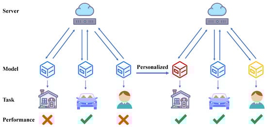
Figure 1.
Schematic diagram of personalized federated learning. On the left, traditional federated learning uses a single model across multiple scenarios, which makes it challenging to address the differences in data distribution among clients. In contrast, the right part shows that personalized federated learning trains distinct models for each client, enabling these client-specific models to perform better on their respective tasks.
2.2. Contrastive Learning
In recent years, contrastive learning techniques have been widely applied in unsupervised learning scenarios and have achieved leading performance in the unsupervised training of deep image models and graph models [29,30,31,32,33]. Many studies focus on training encoders to pull embeddings of similar samples closer while pushing dissimilar samples apart, thereby enhancing model performance. Additionally, since contrastive learning enables federated learning to achieve higher accuracy with less data, there have been many works in recent years combining the two approaches. Model-contrastive federated learning (MOON) [34] introduces model contrastive loss, aiming to align the current local model with the global model while pushing the current local model away from the previous round local model. Federated self-supervised learning (FedSSL) [35] processes unlabeled data collected from edge devices through self-supervised contrastive learning. Prototypical contrastive federated learning (FedProc) [36] uses contrastive loss to align local features with global prototypes, thereby reducing the representation gap, where the global class prototypes are distributed by the server. Bias-reduction federated learning (FedBR) [37] uses contrastive learning to align local and global feature spaces by utilizing local data and globally shared proxy data, thereby reducing the bias in local training. However, previous methods fail to simultaneously enhance the model’s feature extraction capability and personalization performance. We propose a new two-way contrastive learning algorithm. While aligning local and global feature spaces, it increases the distance between the classification layers of local and global models to ensure the improvement of personalized performance.
3. Preliminary
In order to demonstrate the validity of our research question and the proposed method, we provide detailed explanations of some necessary issues in this chapter.
3.1. Problem Formulation
Consider a federated learning system with a total of M devices, denoted by the set . Each device holds a local dataset, which can be represented as
where refers to the d-th input data point, is the associated label, and indicates the total number of samples on device i. The global dataset, formed by combining the datasets from all devices, is denoted as
where N is the overall number of pieces of data across all devices.
The objective of personalized federated learning is to collaboratively train a different model for each client using local datasets without exchanging raw data directly. We define the global loss function as follows:
where denotes the loss function for a single input. For a particular device i, the local loss function is given by
The personalized federated learning problem is then formulated as the following optimization problem:
3.2. Motivation
In machine learning, most models can be divided into two layers: the feature extraction layer and the classification layer. The last layer of the model is generally defined as the classification layer, while the other layers are defined as feature extraction layers. The feature extraction layer is responsible for extracting abstract features from the input data and projecting them into a high-dimensional space. The classification layer is responsible for dividing and classifying the information in this high-dimensional space.
Our approach is based on the conclusion that, in federated learning, the global model’s feature extraction capability is superior to that of the client models, and the performance bottleneck of a single global model lies in its inability to use different classification heads to address the diverse data distributions of individual clients. In Figure 2, we use t-SNE to demonstrate the feature extraction results under different settings, validating the global model’s superior performance in feature extraction. Among them, the results of Figure 2a,b were obtained using the CIFAR-10 [38] with a Dirichlet distribution ().
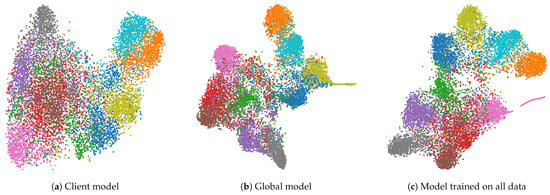
Figure 2.
Visualizations of t-SNE outputs from different models. In it, different colors represent different categories. The “client model” refers to the model trained using only its own partial data in federated learning, the “global model” refers to the server model aggregated from client models, and the “Model trained on all data” refers to the model trained directly using the entire dataset. The feature extraction capability of the global model is significantly stronger than that of the client model and is close to that of the model trained directly on all data.
Existing methods typically focus on processing the feature extraction layer or the classification layer individually, which allows the model to only enhance its feature extraction capability or personalization capability separately, but not both simultaneously. As a result, it is difficult to comprehensively improve the overall performance. Therefore, this paper proposes a novel algorithm that strengthens both the model’s feature extraction capability and personalization capability through a bidirectional contrast approach. Specifically, our method brings the feature extraction representations of the client and global models closer together to enhance the client’s feature extraction ability, while distancing the classification representations of the client and global models to enhance the client’s personalized expression ability.
4. Method
4.1. Framework Overview
Our algorithm consists of two parts: In the first part, we divide the model into the feature extraction layer and the classification layer. The last layer of the model is used as the classification layer, and the remaining layers serve as the feature extraction layers. During training, we collect the outputs of each sample from both layers for training in the next part. The second part involves bidirectional contrastive learning. Based on the high-dimensional representations obtained from the different layers in the first part, we use a contrastive learning method to make the feature extraction layer representation of the client close to that of the global model, while pushing the classification layer representation of the client away from that of the global model. This way, we enhance both the feature extraction capability and personalization of the model. The pseudocode of our algorithm is shown in Algorithms 1 and 2, and the schematic diagram of our algorithm is shown in Figure 3.
| Algorithm 1 FDCL-Server |
Input: global round T, all clients set c, client local steps Q, initial model , dataset size Output: a trained model
|
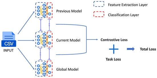
Figure 3.
FDCL framework diagram. In our algorithm, the loss function consists of two parts: one is the contrastive learning loss between layers, and the other is the loss related to the task itself.
| Algorithm 2 FDCL-Client |
Input: all clients c, client learning rate , local epoch E, temerature , client’s dataset , local model w, global model Output: a trained model
|
4.2. Model Partition
Similar to many existing studies, we divide the model architecture into two main components: the feature extraction layer and the classification layer . Specifically, suppose that a model M has a total of N layers, with layers as its encoder; the definition of is as follows:
Similarly, let us assume that the model starts to be a classification layer from the -th layer; then, the definition of is as follows:
In this structure, is responsible for extracting high-level abstract features from the raw input data. These features often contain the key information and patterns of the data, helping the model to understand the core structure of the data. The classification layer , on the other hand, uses the features extracted by to produce the final classification output, mapping these abstract features to specific class labels through a series of operations. We recommend that, in encoder–decoder architectures, the partitioning of and should align with the original architecture’s inherent division. For other architectures, it is advised to designate the final layer as the layer while classifying all preceding layers as layers.
In the following discussion, we denote the output of as , representing the intermediate feature representation obtained from the feature extraction layer. Meanwhile, the output of is denoted as , which represents the final prediction result obtained through the classification layer.
The advantage of this structure lies in the separation of feature extraction and classification tasks, allowing the model to focus more on learning effective feature representations, thereby improving its performance on complex tasks. Additionally, this architecture provides greater flexibility for future task adaptation and model transfer.
4.3. Bidirectional Contrastive Learning
In this section, we introduce the bidirectional contrastive learning component of our model. To enhance feature extraction capabilities and improve personalization, our model performs contrastive learning not only with the global model but also with the previous version of the local model.
We define the components of the models as follows:
- The feature extraction layer of the global model is denoted as , and the classification layer is ;
- The feature extraction layer of the current version of the client model is , and the classification layer is ;
- The feature extraction layer of the previous version of the client model is , and the classification layer is .
The outputs and are named according to the same convention. For example, represents the output of , represents the output of , and so forth for other pairs.
We first compute the loss for the feature extraction layer. Given the powerful feature extraction ability of the global model, the feature extraction layer of the current client model should learn the feature extraction capability of the global model as much as possible. Therefore, our goal is to minimize the distance between and , while maximizing the distance between and . The loss function for the feature extraction layer is as follows:
Here, is a hyperparameter. In order to enhance the personalized performance of the client models, we need to increase the distance between the classification head of each client model and the classification head of the global model while reducing the distance between the model’s classification head and the previous version’s classification head to maintain its performance on the local dataset. Our classification layer loss function is as follows:
Our overall loss function is as follows:
Here, is a given hyperparameter. In Figure 4, we illustrate the differences between FDCL and other methods. By employing the loss function, we further increase the distance between the client and the server based on PFL, thereby enabling the client’s model to approach the local optimal solution more closely.
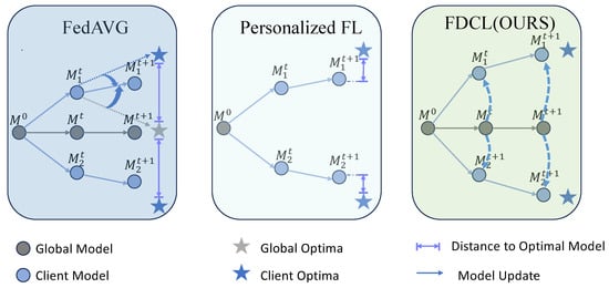
Figure 4.
Comparison between FDCL and other federated learning algorithms. In FedAVG, the update direction of clients is influenced by both local and global optima, and the final aggregated model tends towards global optima, resulting in poor performance of the global model on some clients. In PFL, due to personalized settings, the model performs well on the client side. FDCL enhances the personalization ability of the client through bidirectional contrastive learning, making the client model closer to the local optimal solution.
5. Experiment
In this section, we demonstrate the excellent performance of the FDCL algorithm by running it on different datasets and comparing it with other algorithms under various experimental settings. Additionally, we investigate the impact of different hyperparameters on the performance of the FDCL algorithm. The Dirichlet distribution in this experiment is automatically partitioned using the FLGO framework. By specifying the number of clients, the value of the Dirichlet distribution, and the dataset, FLGO can quickly divide the entire dataset into federated datasets ready for experimentation.
5.1. Experimental Setup
The experimental hardware configuration includes Intel Xeon CPU E5-2690, RTX4090, and 128 GB RAM. The operating system is Ubuntu 20.04.4 LTS. We choose to implement our algorithm through the FLGO [39] framework. The FLGO framework is an efficient and easy-to-use federated learning algorithm framework that supports simulating federated learning under various parameters. We simulated virtual scenes of 20 clients on FLGO to simulate federated learning in real-world scenarios.
Datasets. In this chapter, we selected four commonly used image classification datasets, namely, MNIST [40], Fashion-MNIST [41], CIFAR-10, and CIFAR-100 [38], as well as a graph dataset, MUTAG [42], to evaluate the performance of the algorithm. MNIST is a classic handwritten digit dataset, containing 70,000 grayscale images, each with a resolution of 28 × 28 pixels. The dataset is divided into 60,000 training images and 10,000 testing images, covering 10 digit classes. Fashion-MNIST is a dataset similar to MNIST, containing 70,000 grayscale images of fashion products, with the same resolution of 28 × 28 pixels. The dataset is divided into 10 classes, including clothing, footwear, and other fashion items, with the same number of training and testing images as MNIST. The CIFAR-10 dataset contains 60,000 RGB color images, each with a resolution of 32 × 32 pixels, divided into 10 classes, with 6000 images per class. The dataset consists of 50,000 training images and 10,000 testing images. CIFAR-100 is an extended version of CIFAR-10, containing 60,000 color images with a resolution of 32 × 32 pixels, divided into 100 classes, with 600 images per class. The training and testing sets contain 50,000 and 10,000 images, respectively. The MUTAG dataset comprises 188 nitro compounds, with labels indicating whether each compound is aromatic or heteroaromatic. We visualize the data distributions under different values in Figure 5.
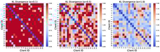
Figure 5.
Visualization of data distribution with different values. We allocated the CIFAR-10 dataset to 20 clients using the Dirichlet distribution with parameters = 0.1, 0.5, and 1.0, and generated a heatmap of the KL divergence between the data distributions of each clients. The redder a grid cell, the greater the disparity between the data distributions, while, the bluer a grid cell, the more similar the data distributions.
To simulate different types of data distributions, we adopted the Dirichlet distribution, which is commonly used in federated learning, as the data partitioning strategy. The Dirichlet distribution is often used as a prior for data distributions to characterize the data distribution across different clients, where the hyperparameter controls the level of uniformity in the data distribution. A larger value of indicates a more uniform distribution, while a smaller value of reflects more complex data heterogeneity. To better simulate the application scenarios of personalized federated learning, we set = 0.1 and = 0.5 to represent cases with severe data heterogeneity and mild data imbalance, respectively.
Models. For all computer vision datasets, a convolutional neural network (CNN) model was used in this paper for pattern recognition. As a fundamental architecture of neural networks, CNN excel at extracting local features from images, making them highly effective for image classification tasks [43,44]. The core idea of CNN is to utilize convolutional layers to extract local features from the input data and to progressively reduce the spatial dimensions of the features through pooling layers, thereby reducing the computational load and enhancing the model’s generalization ability.
The model used in our experiments consists of a feature extractor and a classifier. The feature extractor consists of two convolutional layers, each followed by a ReLU activation function [45] and a 2 × 2 maximum pooling layer. The first convolutional layer uses 32 “5 × 5” convolutional kernels to extract basic features from the input features, and the second convolutional layer uses 64 “5 × 5” convolutional kernels for feature extraction. After feature extraction, the model maps the extracted features onto a 512-dimensional vector through a fully connected layer. This vector is passed through the ReLU activation function and finally converted into the output of the model by another fully connected layer. The mathematical expression of the ReLU function is ReLU(x) = max(x, 0). By introducing this activation function, we can incorporate nonlinearity while mitigating the issues of gradient explosion and vanishing gradients [46,47].
It is worth noting that, in the experimental section, although we only employ this basic CNN for testing, our method is in fact applicable to all models whose final layer can serve as a classification head, such as a fully connected layer. Our approach solely modifies the loss function without altering the model architecture, which ensures its versatility to a certain extent.
Furthermore, for graph datasets, a default Graph Isomorphism Network (GIN) was used in the experiments in [48].
Hyperparameters. In all our experiments, we carefully selected and tuned the hyperparameters to achieve optimal performance. Specifically, the learning rate was set to 0.01, providing a good balance between fast convergence and stability, with a decay rate of 0.999 to gradually reduce the learning rate during training. The batch size was set to 32, a commonly used value that balances computational efficiency and performance. All shared hyperparameters are kept consistent, and, if there are specific hyperparameters, they are set according to the recommended values from the corresponding papers.
For federated learning, we configured the global communication rounds to 100, ensuring sufficient training iterations, with 5 local epochs per round to allow clients to learn from their local data. The client participation rate was set to 50%, meaning that half of the clients participated in each round, balancing communication costs and model performance. Additionally, the hyperparameter was set to 0.1 to regulate the balance between personalization and global model aggregation. The temperature hyperparameter for knowledge distillation was set to 0.5. Finally, the SGD optimizer was used to update the model parameters during training, ensuring efficient learning.
Baselines. To verify the performance of our method in asynchronous environments, we compared it with several classic and advanced federated learning algorithms across multiple datasets. The algorithms compared include FedAVG [13], DITTO [19], MOON [34], FedCP [49], and FedPer [24]. The introductions of these algorithms are as follows:
- FedAVG: FedAVG is a fundamental federated learning algorithm that performs global model averaging updates by training locally on the client and uploading updates to the server;
- DITTO: DITTO achieves fairness and robustness in heterogeneous environments by introducing a globally regularized multi-task learning framework;
- MOON: MOON uses contrastive learning to enhance the representation ability of global models and conducts personalized learning between clients through contrastive loss functions;
- FedPer: FedPer addresses the issue of non-independent and identically distributed data by learning personalized models for each client, thereby improving personalized performance;
- FedCP: FedCP dynamically learns a conditional policy to disentangle global and personalized information from its features, followed by independent processing through a global processing module and a personalized processing module.
In the experimental section, we kept the hyperparameters common to all methods the same, while setting the hyperparameters specific to each algorithm (if any) to the recommended values in the respective papers.
5.2. Performance Comparison
In this section, we conduct experiments on all baseline methods under fixed global rounds and record the final accuracy achieved by each algorithm, as shown in Table 1. Meanwhile, in Figure 6, we also recorded the training curves of all algorithms on different datasets. The experimental results show that, in almost all experimental settings, the final accuracy of our proposed algorithm FDCL is superior to other algorithms. It is noteworthy that, on the CIFAR-100 dataset (with ), our algorithm performs slightly worse than the MOON. Through in-depth analysis, we attribute this phenomenon to the inherent characteristics of our algorithm design: compared to MOON, our method enhances client personalization, which may cause the classification head parameters of individual clients to deviate from the global optimum. In scenarios with weak data heterogeneity (i.e., relatively uniform client data distribution), where the global and local optima exhibit high consistency, this personalization enhancement strategy may lead to a slight performance degradation.

Table 1.
Final accuracy of different algorithms under various settings after 100 epochs. The bold numbers represent the highest values.
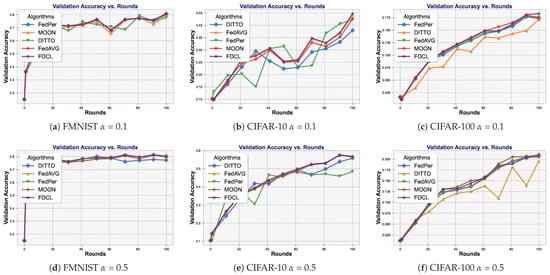
Figure 6.
Algorithm performance comparison on three different datasets.
However, it is crucial to emphasize that personalized federated learning is primarily applied in scenarios with significant data heterogeneity. Therefore, FDCL consistently demonstrates superior performance in real-world applications.
5.3. The Impact of Participation Rate
The participation rate refers to the ratio of the number of clients participating in training during each communication round to the total number of clients. In this section, we investigate the performance of our algorithm under varying client participation rates. Extensive experiments were conducted using our algorithm on the CIFAR-10 dataset with = 0.1 and different participation rates, and the results are presented in Table 2. The performance of all algorithms improves as the participation rate increases. However, our algorithm, FDCL, consistently demonstrates strong performance across different client participation rates, which highlights its robustness to variations in client participation.
Table 2.
Performance comparison under same rounds on CIFAR-10. The bold numbers represent the highest values.
5.4. Effectiveness of the Number of Classification Heads
The number of classification heads refers to the number of layers in . To assess the impact of the number of layers in on the performance of the FDCL algorithm, we conducted experiments using the CIFAR-10 dataset with = 0.1 and evaluated different configurations of . The experimental results, as shown in Figure 7, reveal that the accuracy of the FDCL model is highest when is set to 1. In contrast, when the number of layers in is increased, the algorithm’s performance exhibits a noticeable decline, with accuracy decreasing to varying degrees, depending on the number of layers. This trend suggests that increasing the depth of may negatively impact the model’s generalization ability. Based on these observations, we conclude that setting to 1 is optimal for achieving the best performance of the FDCL algorithm.
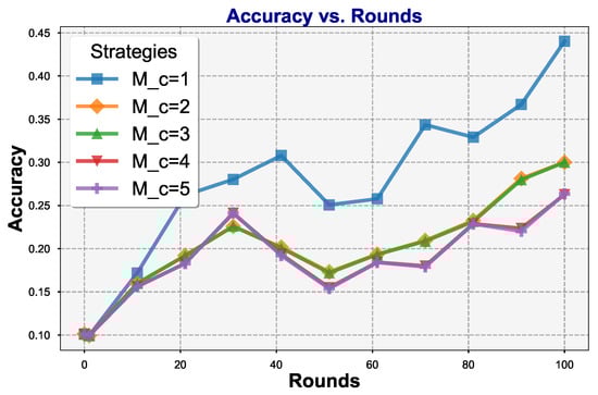
Figure 7.
Comparison of different numbers of classifier heads () on CIFAR-10.
5.5. The Impact of Hyperparameter
The hyperparameter controls the balance between the bidirectional contrastive loss and the total loss. In this section, we conduct extensive experiments to investigate the impact of on algorithm performance and to identify its optimal value. We performed experiments on the FDCL algorithm using different values of on the CIFAR-10 dataset, with the results shown in Table 3. In the experiments, the algorithm achieved the highest accuracy when = 0.1. When the value of either decreased or increased, the accuracy of the algorithm decreased to varying degrees. This is because, when is too small, the effect of bidirectional contrastive learning becomes less pronounced, and the performance approaches that of FedAVG. Conversely, when is too large, bidirectional contrastive learning dominates the training process, reducing the impact of task loss, which leads to suboptimal performance on the dataset. Therefore, we recommend setting to 0.1, as this results in better performance of FDCL.
Table 3.
Performance comparison under the same number rounds on CIFAR-10. The bold numbers represent the highest values.
5.6. The Impact of Local Epochs
Local epochs refers to the number of epochs that selected clients train locally during each communication round in federated learning. In this section, we conducted experiments on the FMNIST datasets with different algorithms and varying local epoch settings to investigate the impact of local epochs on algorithm performance. The experimental results are shown in Figure 8. We observed that appropriately increasing the local epochs within the range of 1 to 10 improved the algorithm’s final accuracy. This is because, when local epochs are too small, local training has not stabilized before the model participates in server aggregation, leading to poorer performance. However, we do not recommend setting a very high number of epochs, as this would significantly increase the federated learning training time and introduce the risk of overfitting in the context of personalized federated learning [50].
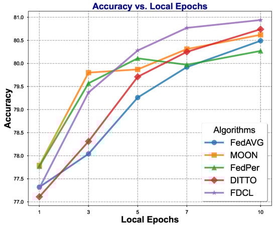
Figure 8.
Comparison of different algorithms running various local epochs.
5.7. Influence of Client Quantity
To investigate the robustness of our method, we also compared its performance with other approaches under varying numbers of clients. In federated learning, increasing the number of clients without expanding the total dataset size leads to a decline in the final model’s accuracy. This occurs because the data volume per client decreases in such scenarios, resulting in a more dispersed distribution of training data, which adversely affects the training process. Our experiments validate this conclusion; the experimental results are shown in the Table 4. Notably, the proposed framework, as a personalized federated learning method, performs well under uneven data distribution and outperforms other personalized federated learning approaches. This advantage stems from our division of the model into two parts, which simultaneously enhances both feature extraction capability and personalization, thereby improving the model’s overall performance.
Table 4.
Results comparison across varying numbers of clients on CIFAR-10. The bold numbers represent the highest values.
5.8. Ablation Study
We conducted an ablation study on the CIFAR-10 and CIFAR-100 datasets using a Dirichlet distribution with = 0.01 to evaluate the impact of different modules. Since a more imbalanced data distribution can better demonstrate the advantages of our proposed method, we adopted this value. The main components of our algorithm are and . Therefore, in this section, we conduct an ablation experiment on these two components. The experimental results are shown in Table 5. Our experiments reveal that incorporating improves the model’s accuracy on CIFAR-10 by 2.24%, while yields a more significant enhancement (36.63→39.45), indicating that plays a more crucial role in feature learning. A similar trend is observed on CIFAR-100. When both and are employed simultaneously, the model achieves optimal performance (CIFAR-10: 40.32%, CIFAR-100: 18.48%), demonstrating their synergistic effect. This is because optimizes feature representation, whereas further refines the classification boundaries.
Table 5.
Ablation experiment results.
6. Analysis
6.1. Communication Overhead
Our method only transmits the model itself during the client–server communication process, with no additional information involved in the transmission, thus introducing no extra communication costs.
6.2. Scalability Under Low-Resource Conditions
Since introducing contrastive learning on the client side increases computational costs, we analyzed the additional overhead that it incurs to evaluate its scalability under low-resource conditions.
We measured the execution time per round for different algorithms under identical conditions, where each round involved 100 clients participating in training, with each client running 5 local epochs. As shown in Table 6, the results demonstrate that, although the introduction of contrastive learning incurs additional computational overhead, the impact remains limited. Thus, our method maintains satisfactory operational efficiency, even in resource-constrained scenarios.
Table 6.
Time required for different algorithms to run one round.
6.3. Convergence Analysis
We provide a detailed convergence analysis for the FDCL algorithm under standard federated learning assumptions.
Consider a federated learning system with K clients, each with a local dataset . The global objective is
where and are the feature extraction and classification layer parameters.
In FDCL, each client optimizes
where balances task and contrastive losses, is the global model, and is the previous local model.
6.3.1. Assumptions
- Smoothness: , , and are L-smooth;
- Strong Convexity: is -strongly convex and is -strongly convex if and are convex;
- Bounded Heterogeneity: ;
- Bounded Contrastive Gradient: .
6.3.2. Local Update
For client k at round t, starting from , perform Q SGD steps with step size :
Using -smoothness,
With ,
By -strong convexity,
After Q steps,
6.3.3. Local Deviation
Since ,
By strong convexity,
6.3.4. Global Aggregation
The global update is
For ,
Compute
6.3.5. Convergence Rate
Let ;
Solve
With ,
Therefore, it can be proven that FDCL is convergent.
7. Conclusions
In this paper, we propose a novel dual-layer bidirectional contrastive federated learning method to address the challenges of data heterogeneity and model personalization in federated learning. By decomposing the model into two layers—the feature extraction layer and the classification layer—and applying bidirectional contrastive learning, our method enhances the feature extraction capabilities of the global model while maintaining strong personalization for individual clients. Experimental results across multiple datasets demonstrate that FDCL outperforms existing federated learning algorithms, such as FedAVG, DITTO, and MOON, in terms of classification accuracy and robustness, particularly under conditions of significant data heterogeneity.
The proposed approach effectively balances the benefits of global model generalization and client-specific personalization, making it a promising solution for real-world federated learning applications. In future work, we will aim to refine our model’s scalability and explore its performance in additional domains, while further optimizing key hyperparameters to enhance both efficiency and accuracy.
Author Contributions
Supervision, F.F.; Writing—original draft, M.L. All authors have read and agreed to the published version of the manuscript.
Funding
This research received no external funding.
Data Availability Statement
The datasets used in this paper are all publicly available datasets, and references have been added. Anyone can conveniently download the datasets used in this paper from the Internet through the reference information.
Conflicts of Interest
The authors declare no conflicts of interest.
References
- Kairouz, P.; McMahan, H.; Avent, B.; Bellet, A.; Bennis, M.; Bhagoji, A.; Bonawitz, K.; Charles, Z.; Cormode, G.; Cummings, R.; et al. Advances and Open Problems in Federated Learning; Georg Thieme: Stuttgart, Germany, 2021; Volume 14, pp. 1–210. [Google Scholar] [CrossRef]
- Liu, J.; Huang, J.; Zhou, Y.; Li, X.; Ji, S.; Xiong, H.; Dou, D. From distributed machine learning to federated learning: A survey. Knowl. Inf. Syst. 2022, 64, 885–917. [Google Scholar] [CrossRef]
- Gao, W.; Xu, G.; Meng, X. FedCon: Scalable and Efficient Federated Learning via Contribution-Based Aggregation. Electronics 2025, 14, 1024. [Google Scholar] [CrossRef]
- Chen, Z.; Zhou, C.; Jiang, Z. One-Shot Federated Learning with Label Differential Privacy. Electronics 2024, 13, 1815. [Google Scholar] [CrossRef]
- Hsu, T.M.H.; Qi, H.; Brown, M. Federated Visual Classification with Real-World Data Distribution. In Proceedings of the Computer Vision—ECCV 2020: 16th European Conference, Glasgow, UK, 23–28 August 2020; Springer: Berlin/Heidelberg, Gernany, 2020; pp. 76–92. [Google Scholar] [CrossRef]
- Koutsoubis, N.; Yilmaz, Y.; Ramachandran, R.P.; Schabath, M.; Rasool, G. Privacy Preserving Federated Learning in Medical Imaging with Uncertainty Estimation. arXiv 2024, arXiv:2406.12815. [Google Scholar]
- Li, Z.; Li, Q.; Zhou, Y.; Zhong, W.; Zhang, G.; Wu, C. Edge-cloud Collaborative Learning with Federated and Centralized Features. In Proceedings of the 46th International ACM SIGIR Conference on Research and Development in Information Retrieval, SIGIR ’23, Taipei, China, 23–27 July 2023; ACM: New York, NY, USA, 2023; pp. 1949–1953. [Google Scholar] [CrossRef]
- Li, Z.; Lin, T.; Shang, X.; Wu, C. Revisiting weighted aggregation in federated learning with neural networks. In Proceedings of the 40th International Conference on Machine Learning, ICML’23, Honolulu, HI, USA, 23–29 July 2023; JMLR.org: Brookline, MA, USA, 2023. [Google Scholar]
- Liu, Y.; Huang, A.; Luo, Y.; Huang, H.; Liu, Y.; Chen, Y.; Feng, L.; Chen, T.; Yu, H.; Yang, Q. FedVision: An Online Visual Object Detection Platform Powered by Federated Learning. arXiv 2020, arXiv:2001.06202. [Google Scholar] [CrossRef]
- Hu, M.; Zhou, P.; Yue, Z.; Ling, Z.; Huang, Y.; Li, A.; Liu, Y.; Lian, X.; Chen, M. FedCross: Towards Accurate Federated Learning via Multi-Model Cross-Aggregation. In Proceedings of the 2024 IEEE 40th International Conference on Data Engineering (ICDE), Utrecht, The Netherlands, 13–16 May 2024; pp. 2137–2150. [Google Scholar] [CrossRef]
- Hu, M.; Cao, Y.; Li, A.; Li, Z.; Liu, C.; Li, T.; Chen, M.; Liu, Y. FedMut: Generalized Federated Learning via Stochastic Mutation. Proc. AAAI Conf. Artif. Intell. 2024, 38, 12528–12537. [Google Scholar] [CrossRef]
- Hu, M.; Yue, Z.; Xie, X.; Chen, C.; Huang, Y.; Wei, X.; Lian, X.; Liu, Y.; Chen, M. Is Aggregation the Only Choice? Federated Learning via Layer-wise Model Recombination. In Proceedings of the 30th ACM SIGKDD Conference on Knowledge Discovery and Data Mining, KDD ’24, Barcelona, Spain, 25–29 August 2024; ACM: New York, NY, USA, 2024; pp. 1096–1107. [Google Scholar] [CrossRef]
- McMahan, H.B.; Moore, E.; Ramage, D.; Hampson, S.; y Arcas, B.A. Communication-Efficient Learning of Deep Networks from Decentralized Data. arXiv 2023, arXiv:1602.05629. [Google Scholar]
- Li, T.; Sahu, A.K.; Zaheer, M.; Sanjabi, M.; Talwalkar, A.; Smith, V. Federated Optimization in Heterogeneous Networks. arXiv 2020, arXiv:1812.06127. [Google Scholar]
- Mendieta, M.; Yang, T.; Wang, P.; Lee, M.; Ding, Z.; Chen, C. Local Learning Matters: Rethinking Data Heterogeneity in Federated Learning. arXiv 2022, arXiv:2111.14213. [Google Scholar]
- Zhang, N.; Li, Y.; Shi, Y.; Shen, J. A CNN-Based Adaptive Federated Learning Approach for Communication Jamming Recognition. Electronics 2023, 12, 3425. [Google Scholar] [CrossRef]
- Zhou, Y.; Duan, G.; Qiu, T.; Zhang, L.; Tian, L.; Zheng, X.; Zhu, Y. Personalized Federated Learning Incorporating Adaptive Model Pruning at the Edge. Electronics 2024, 13, 1738. [Google Scholar] [CrossRef]
- Jiang, Y.; Zhao, X.; Li, H.; Xue, Y. A Personalized Federated Learning Method Based on Knowledge Distillation and Differential Privacy. Electronics 2024, 13, 3538. [Google Scholar] [CrossRef]
- Li, T.; Hu, S.; Beirami, A.; Smith, V. Ditto: Fair and Robust Federated Learning Through Personalization. arXiv 2021, arXiv:2012.04221. [Google Scholar]
- Dinh, C.T.; Tran, N.H.; Nguyen, T.D. Personalized Federated Learning with Moreau Envelopes. arXiv 2022, arXiv:2006.08848. [Google Scholar]
- Fallah, A.; Mokhtari, A.; Ozdaglar, A. Personalized Federated Learning: A Meta-Learning Approach. arXiv 2020, arXiv:2002.07948. [Google Scholar]
- Li, X.; Hu, C.; Luo, S.; Lu, H.; Piao, Z.; Jing, L. Distributed Hybrid-Triggered Observer-Based Secondary Control of Multi-Bus DC Microgrids Over Directed Networks. IEEE Trans. Circuits Syst. I Regul. Pap. 2025, 72, 2467–2480. [Google Scholar] [CrossRef]
- Hu, Z.; Su, R.; Veerasamy, V.; Huang, L.; Ma, R. Resilient Frequency Regulation for Microgrids Under Phasor Measurement Unit Faults and Communication Intermittency. IEEE Trans. Ind. Inform. 2025, 21, 1941–1949. [Google Scholar] [CrossRef]
- Arivazhagan, M.G.; Aggarwal, V.; Singh, A.K.; Choudhary, S. Federated Learning with Personalization Layers. arXiv 2019, arXiv:1912.00818. [Google Scholar]
- Finn, C.; Abbeel, P.; Levine, S. Model-Agnostic Meta-Learning for Fast Adaptation of Deep Networks. arXiv 2017, arXiv:1703.03400. [Google Scholar]
- Zhang, J.; Hua, Y.; Wang, H.; Song, T.; Xue, Z.; Ma, R.; Guan, H. FedALA: Adaptive Local Aggregation for Personalized Federated Learning. Proc. AAAI Conf. Artif. Intell. 2023, 37, 11237–11244. [Google Scholar] [CrossRef]
- Zhang, M.; Sapra, K.; Fidler, S.; Yeung, S.; Alvarez, J.M. Personalized Federated Learning with First Order Model Optimization. arXiv 2021, arXiv:2012.08565. [Google Scholar]
- Yang, M.S.; Sinaga, K.P. Federated Multi-View K-Means Clustering. IEEE Trans. Pattern Anal. Mach. Intell. 2025, 47, 2446–2459. [Google Scholar] [CrossRef] [PubMed]
- Duan, H.; Zhao, N.; Chen, K.; Lin, D. TransRank: Self-Supervised Video Representation Learning via Ranking-Based Transformation Recognition. In Proceedings of the IEEE/CVF Conference on Computer Vision and Pattern Recognition (CVPR), New Orleans, LA, USA, 18–24 June 2022; pp. 3000–3010. [Google Scholar]
- Chen, T.; Kornblith, S.; Norouzi, M.; Hinton, G. A Simple Framework for Contrastive Learning of Visual Representations. arXiv 2020, arXiv:2002.05709. [Google Scholar]
- He, K.; Fan, H.; Wu, Y.; Xie, S.; Girshick, R. Momentum Contrast for Unsupervised Visual Representation Learning. arXiv 2020, arXiv:1911.05722. [Google Scholar]
- Grill, J.B.; Strub, F.; Altché, F.; Tallec, C.; Richemond, P.H.; Buchatskaya, E.; Doersch, C.; Pires, B.A.; Guo, Z.D.; Azar, M.G.; et al. Bootstrap your own latent: A new approach to self-supervised Learning. arXiv 2020, arXiv:2006.07733. [Google Scholar]
- Khosla, P.; Teterwak, P.; Wang, C.; Sarna, A.; Tian, Y.; Isola, P.; Maschinot, A.; Liu, C.; Krishnan, D. Supervised Contrastive Learning. arXiv 2021, arXiv:2004.11362. [Google Scholar]
- Li, Q.; He, B.; Song, D. Model-Contrastive Federated Learning. arXiv 2021, arXiv:2103.16257. [Google Scholar]
- Zhuang, W.; Wen, Y.; Zhang, S. Divergence-aware Federated Self-Supervised Learning. arXiv 2022, arXiv:2204.04385. [Google Scholar]
- Mu, X.; Shen, Y.; Cheng, K.; Geng, X.; Fu, J.; Zhang, T.; Zhang, Z. FedProc: Prototypical Contrastive Federated Learning on Non-IID data. arXiv 2021, arXiv:2109.12273. [Google Scholar] [CrossRef]
- Guo, Y.; Tang, X.; Lin, T. FedBR: Improving Federated Learning on Heterogeneous Data via Local Learning Bias Reduction. arXiv 2023, arXiv:2205.13462. [Google Scholar]
- Krizhevsky, A. Learning Multiple Layers of Features from Tiny Images; Technical Report; University of Toronto: Toronto, ON, Canada, 2009. [Google Scholar]
- Wang, Z.; Fan, X.; Peng, Z.; Li, X.; Yang, Z.; Feng, M.; Yang, Z.; Liu, X.; Wang, C. FLGo: A Fully Customizable Federated Learning Platform. arXiv 2023, arXiv:2306.12079. [Google Scholar]
- Deng, L. The MNIST Database of Handwritten Digit Images for Machine Learning Research. IEEE Signal Process. Mag. 2012, 29, 141–142. [Google Scholar] [CrossRef]
- Xiao, H.; Rasul, K.; Vollgraf, R. Fashion-MNIST: A Novel Image Dataset for Benchmarking Machine Learning Algorithms. arXiv 2017, arXiv:1708.07747. [Google Scholar]
- Debnath, A.K.; de Compadre, R.L.L.; Debnath, G.; Shusterman, A.J.; Hansch, C. Structure-activity relationship of mutagenic aromatic and heteroaromatic nitro compounds. Correlation with molecular orbital energies and hydrophobicity. J. Med. Chem. 1991, 34, 786–797. [Google Scholar] [CrossRef]
- Krizhevsky, A.; Sutskever, I.; Hinton, G.E. ImageNet Classification with Deep Convolutional Neural Networks. In Proceedings of the Advances in Neural Information Processing Systems, Lake Tahoe, NV, USA, 3–6 December 2012; Pereira, F., Burges, C., Bottou, L., Weinberger, K., Eds.; Curran Associates, Inc.: Red Hook, NY, USA, 2012; Volume 25. [Google Scholar]
- Simonyan, K.; Zisserman, A. Very Deep Convolutional Networks for Large-Scale Image Recognition. arXiv 2014, arXiv:1409.1556. [Google Scholar] [CrossRef]
- Glorot, X.; Bordes, A.; Bengio, Y. Deep Sparse Rectifier Neural Networks. In Proceedings of the Fourteenth International Conference on Artificial Intelligence and Statistics, Fort Lauderdale, FL, USA, 11–13 April 2011; Volume 15, pp. 315–323. [Google Scholar]
- Song, L.; Fan, J.; Chen, D.R.; Zhou, D.X. Approximation of Nonlinear Functionals Using Deep ReLU Networks. arXiv 2023, arXiv:2304.04443. [Google Scholar] [CrossRef]
- Daubechies, I.; DeVore, R.; Foucart, S.; Hanin, B.; Petrova, G. Nonlinear Approximation and (Deep) ReLU Networks. arXiv 2019, arXiv:1905.02199. [Google Scholar] [CrossRef]
- Xu, K.; Hu, W.; Leskovec, J.; Jegelka, S. How Powerful are Graph Neural Networks? In Proceedings of the International Conference on Learning Representations, New Orleans, LA, USA, 6–9 May 2019. [Google Scholar]
- Zhang, J.; Hua, Y.; Wang, H.; Song, T.; Xue, Z.; Ma, R.; Guan, H. FedCP: Separating Feature Information for Personalized Federated Learning via Conditional Policy. In Proceedings of the 29th ACM SIGKDD Conference on Knowledge Discovery and Data Mining, KDD ’23, Long Beach, CA, USA, 6–10 August 2023; ACM: New York, NY, USA, 2023; pp. 3249–3261. [Google Scholar] [CrossRef]
- Karimireddy, S.P.; Kale, S.; Mohri, M.; Reddi, S.J.; Stich, S.U.; Suresh, A.T. SCAFFOLD: Stochastic controlled averaging for federated learning. In Proceedings of the 37th International Conference on Machine Learning, ICML’20, Vienna, Austria, 12–18 July 2020; JMLR.org: Brookline, MA, USA, 2020. [Google Scholar]
Disclaimer/Publisher’s Note: The statements, opinions and data contained in all publications are solely those of the individual author(s) and contributor(s) and not of MDPI and/or the editor(s). MDPI and/or the editor(s) disclaim responsibility for any injury to people or property resulting from any ideas, methods, instructions or products referred to in the content. |
© 2025 by the authors. Licensee MDPI, Basel, Switzerland. This article is an open access article distributed under the terms and conditions of the Creative Commons Attribution (CC BY) license (https://creativecommons.org/licenses/by/4.0/).