Visual Information Decoding Based on State-Space Model with Neural Pathways Incorporation

Abstract

In contemporary visual decoding models, traditional neural network-based methods have made some advancements; however, their performance in addressing complex visual tasks remains constrained. This limitation is primarily due to the restrictions of local receptive fields and their inability to effectively capture visual information, resulting in the loss of essential contextual details. Visual processing in the brain initiates in the retina, where information is transmitted via the optic nerve to the lateral geniculate nucleus (LGN) and subsequently progresses along the ventral pathway for layered processing. Unfortunately, this natural process is not fully represented in current decoding models. In this paper, we propose a state-space-based visual information decoding model, SSM-VIDM, which enhances performance in complex visual tasks by aligning with the brain’s visual processing mechanisms. This approach overcomes the limitations of traditional convolutional neural networks (CNNs) regarding local receptive fields, thereby preserving contextual information in visual tasks. Experimental results demonstrate that the state-space-based visual information decoding model proposed in this study outperforms traditional decoding models in terms of performance and exhibits higher accuracy in image recognition tasks. Our research findings suggest that the visual decoding model, which is based on the lateral geniculate nucleus and the ventral pathway, can enhance decoding performance.

1. Introduction

The research on visual information decoding aims to establish a mapping relationship between the functional magnetic resonance imaging (fMRI) voxel responses of the visual cortex and natural image stimuli [1]. This mapping allows for the analysis of visual information processed by subjects while viewing natural images, based on the activity of fMRI voxels in the brain’s visual cortex. The objective of this research is to explore and elucidate how the neural activity in the visual cortex decodes and represents the content of visual input, thereby enhancing our understanding of the brain’s mechanisms for processing visual information [2,3]. Current visual decoding models primarily rely on deep neural network (DNN) methods. However, these models often overlook critical components in the visual information transmission process, which adversely affects their decoding capabilities and accuracy.

With the rapid advancement of machine learning, deep learning models for visual information decoding have demonstrated significant potential across various applications. The perception of visual information is typically reflected in multiple aspects, including the brain’s response to visual stimuli, eye movements, and facial expressions. Deep learning models can extract latent features from these multimodal data, enabling accurate decoding and reconstruction of visual scenes. In recent years, researchers have increasingly applied deep learning techniques to the field of visual information decoding, achieving substantial progress. The study by James V. Haxby et al. [4] showed that the functional architecture of object visual pathways in the human brain exhibits significant complexity in the response patterns of the ventral temporal lobe. Kamitani and Tong et al. [5] conducted further research by using stripes with different directions for visual stimulation. They successfully classified multiple different stripe stimuli correctly using fMRI signals generated by visual stimuli.

Vision is the most crucial means by which humans comprehend the external world [6,7]. Through the visual system, individuals can better interpret and interact with their surroundings. Numerous studies in the field of neuroscience have indicated that the processing of visual information in primates exhibits hierarchical characteristics [8,9]. The human visual system primarily consists of structures such as the eyes, optic nerve, lateral geniculate body, and the visual cortex of the brain. Visual information is projected onto the retina via the eyes, and the visual information received by the retina first passes through the LGN before being relayed to the visual cortex. The ventral pathway within the visual cortex plays a vital role in object recognition and semantic understanding [10], and its collaboration with other neural pathways forms a comprehensive mechanism for processing visual information in the brain [11]. Furthermore, existing research has investigated the mechanisms of visual information processing in the brain by developing relevant computational models. However, current decoding models have not completely captured the hierarchical representation of visual regions, nor have they fully elucidated the interactions between LGN and the ventral pathways.

In recent years, deep learning has made significant advancements in the fields of nuclear magnetic resonance spectroscopy (NMR) and magnetic resonance imaging (MRI). Deep learning models, with their robust feature extraction and pattern recognition capabilities, greatly enhance the processing efficiency and analytical accuracy of NMR data. Some studies use CNN to rapidly analyze complex NMR spectra, enabling the automatic identification and classification of spectral peaks. Compared to traditional methods, this approach significantly reduces analysis time and improves result accuracy [12]. In MRI research, researchers integrate interpretability methods with neural network models to enhance the analysis of how the brain processes emotional, visual, and other types of information. This approach not only clarifies the underlying mechanisms but also identifies brain regions associated with emotional perception and psychological activity, offering new insights into the brain’s operational principles [13,14]. For instance, leveraging deep learning models, researchers have successfully predicted human emotional states and, for the first time, decoded specific neural signals related to behavior in the brain activity of animals, such as dogs. This has revealed differences in how various species perceive the world [15]. Furthermore, deep learning techniques can restore or generate image content linked to brain activity data, aiding doctors in more accurately diagnosing brain diseases and formulating treatment plans [16,17]. These advancements address the limitations of traditional methods, allowing MRI to play a more significant role in uncovering the mysteries of the brain and enhancing clinical applications, thereby providing more efficient and intelligent tools for neuroscience research and medical diagnosis.

In this paper, we propose a state space model-based visual information decoding model (SSM-VIDM) designed to address the inadequate consideration of the synergistic effects of visual information processing pathways in existing research. Traditional methods often fail to fully integrate the mutual cooperation among different neural pathways, resulting in limitations in understanding the mechanisms of visual information processing. SSM-VIDM constructed a neural network model that follows biological principles by combining the characteristics of neural pathways, reducing the significant differences in operational mechanisms between traditional artificial neurons and real biological neurons. This model is constructed based on a state space model and adopts a multi-path scanning method, which can simultaneously obtain visual information from multiple angles, thus better capturing local and global features, compensating for the limitations of traditional convolutional neural networks in local receptive fields, and avoiding the loss of contextual information. SSM-VIDM simulated the complex response of the LGN to input images through dynamic modeling, considering the interactions between neurons, including both inhibition and excitation. Additionally, we compared SSM-VIDM with traditional neural networks in terms of decoding accuracy and image recognition performance. The experimental results indicate that SSM-VIDM demonstrates a high degree of similarity in decoding tasks and significantly outperforms traditional neural network models in image recognition accuracy, thereby highlighting its exceptional performance. This study combines neuroscience and deep learning techniques to deepen our understanding of the visual processing mechanisms in the brain while providing new ideas and methods for the development of brain-inspired intelligent systems. Through this interdisciplinary exploration, we hope to reveal how the brain efficiently decodes and processes visual information, providing theoretical support and practical guidance for building more accurate visual decoding models in the future.

2. Related Work

In the field of neuroscience research, the analysis of visual information through neural signal transmission pathways has garnered significant attention from the academic community in recent years. With advancements in imaging technology and data processing methods, the accuracy and resolution of visual information have improved markedly. By employing sophisticated algorithms, researchers can correlate visual image content with variations in neural signals. This not only enhances our understanding of how the brain processes visual information but also offers new insights into the study of perception and memory formation processes [18]. This section reviews relevant work from two perspectives: deep learning and the modeling of biological visual systems, as well as visual information decoding based on neural networks.

2.1. Deep Learning and Modeling of Biological Vision Systems

In recent years, significant breakthroughs have occurred in the application of deep learning to model biological visual systems, particularly in the realm of deep CNNs. CNNs, which are widely utilized deep learning models in image processing, were inspired by the research findings of biologists David Hubel and Torsten Wiesel. Their work demonstrated that the visual cortex of cats possesses a specific hierarchical structure and local perceptual capabilities when processing visual information [19]. This inspiration has transformed CNN into a powerful tool for processing visual information, particularly in modeling biological visual systems, and it demonstrates immense potential.

On this basis, Zhou et al. [20] proposed a lightweight anomaly detection model that integrates graph neural network (GNN) and knowledge distillation techniques. This model effectively extracts features through a graph network reconstruction strategy, utilizing a Graph Attention Network and a Multi-Layer Perceptron. The experimental results indicate that deep learning techniques, particularly when integrated with graph neural networks, can significantly enhance the efficiency and accuracy of visual information processing in practical applications. Chen et al. [21] introduced a Multi-Center Edge Federated Learning framework, which significantly enhances the model’s fault tolerance, accuracy, convergence speed, and robustness by deploying multiple global aggregation centers at the edge, rather than relying on a traditional central server architecture. Additionally, Chen et al. [22] proposed a method for fusing public and expert information based on sentiment analysis and intuitionistic fuzzy numbers. This approach further explores the potential of deep learning in integrating multi-source data and enhancing group decision-making through advanced information fusion technology. Additionally, Zhang et al. [23] proposed an Internet of Things security framework called AntiConcealer, which employs edge artificial intelligence to model attack patterns using multivariate Hawkes processes and groups hidden behaviors through a non-negative weighted influence matrix, thereby verifying the framework’s effectiveness and reliability in identifying attacker behavior. This method significantly enhances the security of IoT systems and fully showcases the immense potential of deep learning in practical applications. Li et al. [24] introduced an end-to-end latency and packet loss analysis framework for body-to-body networks in two-dimensional regions. This framework enhances the accuracy of network performance analysis by thoroughly assessing latency and packet loss rates, thereby offering technical support for the optimization of IoT and communication systems.

These studies not only offer innovative approaches for decoding brain signals but also facilitate the extensive application of deep learning in modeling the biological visual system. Additionally, methods such as the Proportional Interval Type-2 Hesitation Fuzzy Set [25] and the artificial intelligence resource scheduling framework [26] have introduced new research directions for visual information decoding.

Despite significant advancements in visual information processing through deep learning models, several challenges remain. For instance, in complex environments, the recognition accuracy of these models often experiences considerable fluctuations, accompanied by issues of insufficient robustness and high energy consumption [27,28]. In recent years, researchers have increasingly focused on developing computational models that more closely mimic the visual information processing mechanisms of the human brain to address these challenges. In 2024, Liu et al. [29] introduced a visual state space model known as VMamba. This model leverages the strengths of the visual transformer while reducing computational complexity to a linear scale. To enhance the understanding of two-dimensional images, VMamba incorporates the Cross Scan Module (CSM), which transforms two-dimensional image data into one-dimensional sequences, effectively capturing the global features of the images. The SSM-VIDM proposed in this paper leverages the characteristics of the state space model to extract global features from complex images, thereby enhancing the robustness of the decoding model.

2.2. Visual Information Decoding Based on Neural Networks

Artificial neural networks (ANNs) have become essential tools for studying the operational principles of biological visual systems. Numerous studies have developed computational models that more closely resemble the visual information processing mechanisms of the brain by analyzing brain activity data. Early research primarily focused on utilizing fMRI data to decode the brain’s visual activity, aiming to reconstruct the images or scenes viewed by subjects. For instance, Norman et al. [3] collected brain responses from subjects viewing various visual images using fMRI technology and successfully completed the image classification task by training a support vector machine model.

Many studies have made significant progress in decoding visual information. Schoenmakers and his team [30] developed a linear model for reconstructing handwritten letters, achieving commendable results. Cowen et al. [31] integrated partial least squares regression with principal component analysis to successfully reconstruct facial images observed by subjects from fMRI data. Güçlütürk et al. [32] proposed a decoding model based on generative adversarial networks, which further enhanced the reconstruction quality. Shen et al. [33] employed DNN and incorporated prior knowledge of natural images to successfully reconstruct a series of natural images from the ImageNet dataset by optimizing their model.

Kay et al. [34] developed an analytical model to study how the brain processes visual information, which was experimentally validated by inputting various types of images. Then, by comparing the predicted results of the model with the actual monitored brain signals, researchers can systematically identify which images have a higher likelihood of triggering specific brain signals. Through this comparative analysis, they can identify which image features are more likely to trigger specific brain activation phenomena, which also reveals the correlation between visual stimuli and human brain responses. Song et al. [35] proposed a new method for classifying fMRI data, using voxel selection techniques to classify fMRI data, and compared the classification performance of this method with support vector machine models. Fujiwara et al. [36] proposed a bidirectional generative codec model, which uses Bayesian canonical correlation analysis. This model can not only predict the brain’s response to visual images but also deduce visual images from the brain’s response. Horikawa et al. [37] proposed a new feature decoder, which is trained using brain signals and image features. The image features are actually obtained through convolutional neural networks, and the trained feature decoder can use brain signals to predict the corresponding image feature data. Then, the predicted image features are compared with the features of the candidate images one by one, and the most matching image is selected based on their correlation. Wen et al. [28] first extracted intermediate features from DNN and then used the obtained image features to accurately encode and decode natural image stimuli. Du et al. [38] proposed a structured neural information decoding method that deeply explores the similarities and connections between some current computer vision models and human brain visual pathways in hierarchical feature expression through multitask feature decoding. The existing visual information decoding models have demonstrated potential in the field of visual information decoding, but they also exhibit significant limitations. The current model fails to fully utilize the physiological feature of the brain’s visual pathway, leading to deficiencies in interpretability and decoding accuracy. Therefore, the SSM-VIDM proposed in this paper develops a decoding model that leverages the physiological characteristics of the brain’s visual pathway, thereby enhancing both interpretability and decoding accuracy.

3. Method

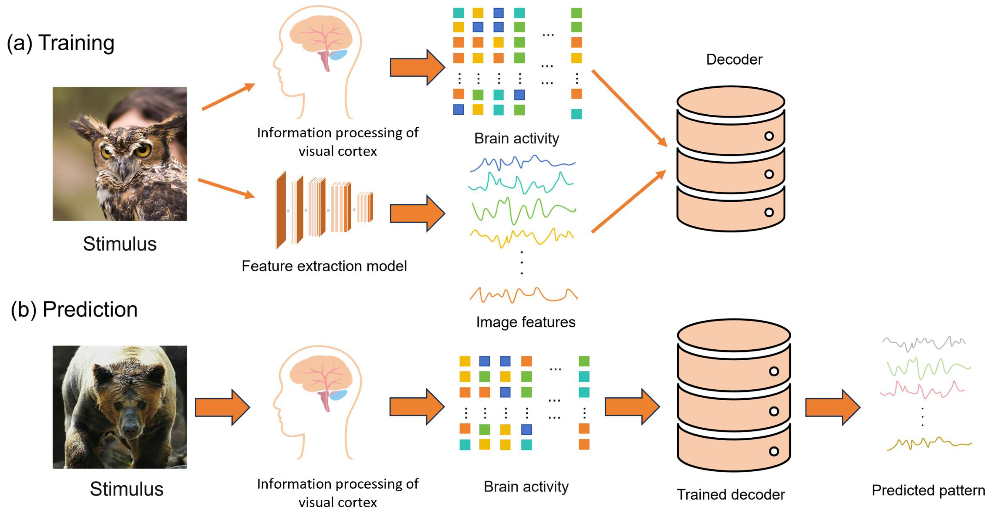
3.1. Visual Information Decoding Process

In this paper, we employ a linearized decoding method to construct a visual information decoding model based on state space. The visual information decoding model consists of two primary processes: training and prediction. The specific methodologies are summarized as follows, with Figure 1 illustrating the entire decoding process. The training process is depicted in Figure 1a. Initially, the image stimuli pass through the brain’s visual cortex and the visual feature extraction model, generating brain activity voxels and image features. Subsequently, these two sets of features are matched one by one to train the linear decoder. The prediction process is illustrated in Figure 1b. First, the image stimuli traverse the visual cortex to produce active voxels, which are then input into the trained decoder to predict image features. The correlation between the decoding model and various visual regions is established by comparing the predicted image features with the actual features. The following chapters will provide a detailed introduction to each step.

3.2. Feature Extraction Model

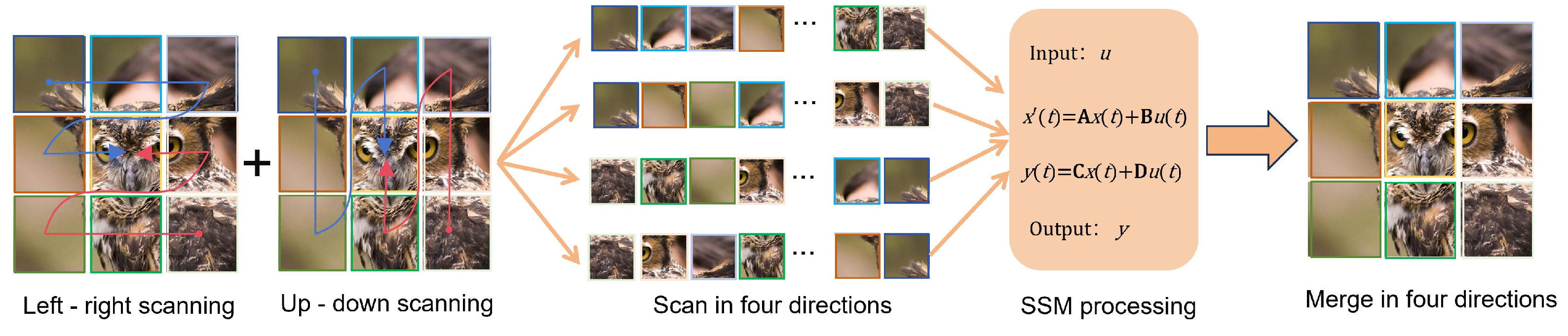
3.2.1. Visual Information Decoding Model Based on State Space Model

The recognition of scenes and objects by humans primarily depends on the collaboration between the LGN and the ventral visual pathway. The transmission pathway of visual information in the brain is illustrated in Figure 2a. Consequently, to develop an effective decoding model, it is essential to align it closely with the physiological mechanisms of the brain’s visual pathway. Furthermore, some decoding models struggle to accurately capture the intricate relationship between visual stimuli and brain responses, leading to limitations in interpretability and decoding accuracy. The SSM, as a powerful analytical tool, can represent the inherent dynamic changes and uncertainties in a system. They have been extensively utilized in fields such as time series analysis and signal processing. In the context of visual information decoding, the incorporation of state space models not only facilitates the understanding of the complex relationship between visual stimuli and neural activity but also accommodates dynamic changes across various time scales. The fundamental concept of this model is to interpret visual information as a dynamic system, where visual stimuli act as inputs and visual features function as outputs. By constructing a state space model that encompasses state variables and observation variables, it is possible to achieve accurate decoding of visual information.

Based on the content presented above, this article proposes a visual information decoding model known as the SSM-VIDM (visual information decoding model based on the state space model), which is grounded in the state space model framework. The structure of the model is illustrated in Figure 2b. The primary objective of the SSM-VIDM is to establish a dynamic correlation between visual stimuli and brain activity. In its design, the model incorporates the physiological characteristics of the human brain when processing image signals and employs a state space model to analyze the complex interrelationships between stimulus signals and neural responses. A distinctive feature of the SSM-VIDM model is its enhanced simulation of the specific processes involved in the LGN when processing visual information. This is achieved by introducing a CSM [29] to simulate the visual processing flow of the LGN. The CSM is utilized in subsequent analysis modules, including the LGN, V1, V2, V4, and IT blocks. The specific parameters are detailed in

Table 1. SSM-VIDM architecture parameters.

Stage	Operation	Output Size
Input		$224\times 224\times 3$
LGN	csm	$224\times 224\times 3$
V1	conv $7\times 7$, stride = 2, padding = 3	$112\times 112\times 64$
	conv $3\times 3$, stride = 1, padding = 1	$112\times 112\times 64$
	csm	$112\times 112\times 64$
V2	conv $1\times 1$	$112\times 112\times 96$
	conv $3\times 3$, stride = 2, padding = 1	$56\times 56\times 96$
	conv $1\times 1$	$56\times 56\times 256$
	csm	$56\times 56\times 256$
V4	conv $1\times 1$	$56\times 56\times 192$
	conv $3\times 3$, stride = 2, padding = 1	$28\times 28\times 192$
	conv $1\times 1$	$28\times 28\times 512$
	csm	$28\times 28\times 512$
IT	conv $1\times 1$	$28\times 28\times 768$
	conv $3\times 3$, stride = 2, padding = 1	$14\times 14\times 768$
	conv $1\times 1$	$14\times 14\times 1536$
	csm	$14\times 14\times 1536$
	avgpool	$1\times 1\times 1536$
	flatten	1536
	Linear	1000

. The Cross Scan Module simulates the processing flow of visual information in the brain through multi-path scanning, allowing for the simultaneous acquisition of information from various perspectives. This processing method enables the network to capture both local and global information concurrently, thereby compensating for the limitations associated with the local receptive fields of CNNs. Unlike the layer-by-layer processing characteristic of CNNs, the Cross Scan Module permits the system to scan from multiple angles simultaneously, mitigating the issue of contextual information loss that may arise with traditional CNN architectures. In the image feature extraction component of the decoding model, this paper employs a trained SSM-VIDM to extract visual features from image stimuli as they pass through the V1, V2, V4, and IT blocks, providing multi-level neural representations for subsequent experiments.

In the field of visual information decoding research, SSM is a powerful tool with distinct advantages. SSM can essentially be classified as a linear time-invariant (LTI) system. Its core function involves establishing a mapping relationship between the input and output by concealing the state $x\left(t\right)$. The input $u\left(t\right)$ typically consists of a carefully preprocessed feature vector derived from a visual image within a scene. The output $y\left(t\right)$ represents the visual feature representation that has been decoded following model processing. These relationships are generally expressed as linear ordinary differential equations, as illustrated below.

$$\begin{array}{cc}\hfill x^{\prime }\left(t\right)& =\mathbf{A}x\left(t\right)+\mathbf{B}u\left(t\right)\hfill \\ \hfill y\left(t\right)& =\mathbf{C}x\left(t\right)+\mathbf{D}u\left(t\right)\hfill \end{array}$$

(1)

where A, B, C, and D are weighted parameters.

Due to the predominance of digital systems in the current computing environment being mostly digital systems, continuous-time SSM cannot be directly applied, making discretization a necessary step. The discretization process begins by solving the differential equations of the SSM to obtain analytical solutions. Concretely, Equation (1) can be expressed as

$$x\left(t_b\right)=e^{\mathbf{A}(t_b-t_a)}x\left(t_a\right)+e^{\mathbf{A}(t_b-t_a)}{\int }_{t_a}^{t_b}\mathbf{B}\left(\tau \right)u\left(\tau \right)e^{-\mathbf{A}(\tau -t_a)}d\tau$$

(2)

This analytical solution describes the evolution of the hidden state from the initial time $t_a$ to the final time $t_b$ within the interval $[t_a,t_b]$, illustrating both state transitions and the cumulative effects of the input. Subsequently, by introducing a fixed sampling interval $\mathrm{\Delta }t$, the continuous-time model is discretized, yielding the following discrete-time expression

$$x_b=e^{\mathbf{A}({\mathrm{\Delta }}_a+\cdots +{\mathrm{\Delta }}_{b-1})}\left(x_a+\sum _{i=a}^{b-1}{\mathbf{B}}_i{u}_i{e}^{-\mathbf{A}({\mathrm{\Delta }}_a+\cdots +{\mathrm{\Delta }}_i)}{\mathrm{\Delta }}_i\right)$$

(3)

To facilitate understanding and analysis, by setting $b=a+1$, Equation (3) can be rewritten as

$$\begin{array}{cc}\hfill x_{a+1}& =e^{\mathbf{A}{\mathrm{\Delta }}_a}{x}_a+{\mathbf{B}}_a{\mathrm{\Delta }}_a{u}_a\hfill \end{array}$$

(4)

$$\begin{array}{cc}\hfill & ={\overline{\mathbf{A}}}_a{x}_a+{\overline{\mathbf{B}}}_a{u}_a\hfill \end{array}$$

(5)

where ${\overline{\mathbf{A}}}_a=e^{\mathbf{A}{\mathrm{\Delta }}_a}$ is highly consistent with the discretization result of the Zero-Order Hold (ZOH) method, and ${\overline{\mathbf{B}}}_a={\mathbf{B}}_a{\mathrm{\Delta }}_a$ is approximately the first-order Taylor expansion of the corresponding term in ZOH. This indirectly verifies the rationality and effectiveness of the discretization method.

The Selective Scan mechanism is fundamental to our approach, addressing the shortcomings of traditional LTI SSMs. In particular, we configure the weight matrix $\mathbf{B}$ in Equations (2) and (3) (likewise for matrices $\mathbf{C}$, $\mathbf{D}$, and the time interval $\mathrm{\Delta }$) to be input-dependent. However, this makes the model time-varying, and computational efficiency becomes a major issue, as convolution operations do not support dynamic weights, and the old calculation methods can no longer be used. Nevertheless, if a recurrence relation for $h_b$ in Equation (3) can be found, efficient computation can still be achieved. Specifically, we denote $e^{\mathbf{A}({\mathrm{\Delta }}_a+\cdots +{\mathrm{\Delta }}_{i-1})}$ as ${\rho }_i^{\mathbf{A},a}$, and then its recurrence relation can be written as

$$p_i^{\mathbf{A},a}=e^{\mathbf{A}{\mathrm{\Delta }}_{i-1}}{p}_{i-1}^{\mathbf{A},a}$$

(6)

For the second term in Equation (3), we also have the following calculation process.

$$\begin{array}{cc}\hfill p_b^{\mathbf{B},a}& =e^{\mathbf{A}({\mathrm{\Delta }}_a+\cdots +{\mathrm{\Delta }}_{b-1})}\sum _{i=a}^{b-1}{\mathbf{B}}_i{u}_i{e}^{-\mathbf{A}({\mathrm{\Delta }}_a+\cdots +{\mathrm{\Delta }}_i)}{\mathrm{\Delta }}_i\hfill \end{array}$$

(7)

$$\begin{array}{cc}\hfill & =e^{\mathbf{A}{\mathrm{\Delta }}_{b-1}}{p}_{b-1}^{\mathbf{B},a}+{\mathbf{B}}_{b-1}{u}_{b-1}{\mathrm{\Delta }}_{b-1}\hfill \end{array}$$

(8)

With the relationships derived from Equations (6) and (7), we can use the Parallel Associative Scan algorithm to efficiently compute $x_b=p_b^{\mathbf{A},a}{x}_a+p_b^{\mathbf{B},a}$.

LGN neurons exhibit selectivity for the direction of visual stimuli, demonstrating sensitivity to edges in horizontal, vertical, and diagonal orientations. CSM employs a multi-path scanning strategy (see Figure 3) to decompose the input image into feature sequences across various directions, akin to the parallel decoding of multi-directional visual signals by LGN neurons. In this manner, CSM effectively replicates the efficient decoding of multi-directional information by LGN neurons during the early stages of visual processing.

We evaluate the performance of SSM-VIDM on ImageNet-1K [39]. The model is trained from scratch for 200 epochs with a batch size of 512. We use the Adam optimizer with an initial learning rate of $5\times {10}^{-4}$, decayed via a cosine annealing schedule without restarts. The optimizer parameters are set as ${\beta }_1=0.9$ and ${\beta }_2=0.999$, with a weight decay of $1\times {10}^{-4}$ applied to all learnable parameters. A linear learning rate warm-up is conducted over the first 15 epochs, gradually increasing from $1\times {10}^{-5}$ to the initial rate. Standard data augmentation techniques are employed, including random resized cropping, horizontal flipping, and color jittering. To prevent overfitting, label smoothing ($ϵ=0.1$) and stochastic depth (with survival probabilities linearly decayed from 1.0 to 0.8 for deeper layers) are used for regularization. Gradient clipping by norm with a threshold of $1.0$ is applied to stabilize training, and the exponential moving average (EMA) of model weights is maintained with a decay factor of $0.9999$ to improve inference stability. No additional training tricks are used, ensuring a focused and reproducible experimental setup. All hyperparameters are tuned on the validation set to maximize the model’s generalization performance. The trained SSM-VIDM is utilized for subsequent image feature extraction.

3.2.2. Visual Information Decoding Model Based on Convolutional Neural Network

The CNN is a deep learning algorithm particularly well suited for processing grid-structured data, such as images and videos. CNNs mimic the mechanisms of the biological visual system to process images and recognize features. In this paper, we selected the classic convolutional neural network, AlexNet [40], as the image feature extractor, referring to it as CNN-VIDM for the purposes of our subsequent research. The CNN-VIDM comprises five convolutional layers and three fully connected layers, designed to extract multi-level features from images. We focus on extracting image features from the first and fifth convolutional layers, as well as the fully connected layers of the first and third layers, from the trained model. The features derived from these layers exhibit strong representational power and capture image information at various levels. Matthew et al. [41] proposed a visualization technique using deconvolution networks, which they combined with the activation maximization technique to assess the capability of deep network features in capturing various levels of image information.

We also benchmarked the model against GoogLeNet [42] and ResNet-18 [43]. GoogLeNet innovatively introduces the Inception module, which captures multi-dimensional features of images through parallel multi-scale convolution and pooling operations. It employs global average pooling instead of fully connected layers to reduce the number of parameters, enhancing the network’s width and representation capability. ResNet-18, a lightweight version of the residual network series, boasts a core advantage in its residual connection structure. By learning the residuals between input and output, it addresses the issues of gradient vanishing and degradation that arise as the depth of traditional CNNs increases. For our subsequent experiments, we primarily extract image features from the last convolutional layer of these two networks.

In our experiment, we utilized pre-trained AlexNet, GoogleLeNet, and ResNet-18 models from PyTorch’s torchvision.models module, all of which were trained on the ImageNet dataset. These models can be directly employed without the need for retraining, ensuring consistent validation performance in large-scale visual tasks. We used these trained models for feature extraction.

3.3. Visual Feature Decoder

We constructed a visual feature decoder that predicts the feature vectors of visual objects from fMRI activity using a linear regression function. The decoder is represented by the following formula.

$$y\left(x\right)=\sum _{i=1}^n{w}_i{x}_i+b,$$

(9)

where y represents the visual feature vector, $x_i$ denotes the fMRI response value of voxel, b is the bias term, $w_i$ is the weight of the i-th voxel, and n indicates the number of voxels. We trained a visual feature decoder to predict feature vectors of a single feature type for a given fMRI sample in the training image. For the test dataset, the corresponding categories of fMRI samples were averaged during the experiment (35 samples in the test image session and 10 samples in the image experiment) to enhance the signal-to-noise ratio of the fMRI signals. By utilizing the trained visual decoder, we can predict the feature vectors of fMRI samples in the test set.

3.4. Model Effectiveness Evaluation

3.4.1. Decoding Effectiveness Evaluation

In this paper, we demonstrate the performance of the decoding model by evaluating it through the calculation of the Pearson correlation coefficient. This coefficient measures the relationship between the visual features predicted by the model and the actual features. This calculation is performed as follows:

$$\rho =cor(\gamma ,\widehat{\gamma })={\displaystyle \frac{Cov(\gamma ,\widehat{\gamma })}{{\sqrt{Var\left(\gamma \right)·Var\left(\widehat{\gamma }\right)}}^{\prime }}},$$

(10)

where $\rho$ represents the Pearson correlation coefficient between the true feature $\gamma$ and the predicted feature $\widehat{\gamma }$. To assess whether the correlation value $\rho$ is statistically significant, this experiment employed a data permutation test. The specific procedure is as follows: randomly shuffle the correspondence between actual features and predicted results and then recalculate the correlation values between the two. This permutation process must be repeated 1000 times to obtain a numerical distribution that reflects the absence of actual correlation. We define $\rho$ = 0.25 (p < 0.001, randomized test) as the effective threshold, allowing us to conclude that there is indeed a similarity between the predicted results and the true features. At this point, the model can interpret the data features.

3.4.2. Identification Accuracy Evaluation

To assess the practical utility of the model, this paper conducted an evaluation of image recognition accuracy. The decoding model analyzes the image features corresponding to all brain responses in the test set and identifies the perceived images of the subjects by calculating the correlation coefficient between the actual features of the images and the predicted image features. As illustrated in Figure 4, the decoding model predicts brain responses to derive the anticipated features of the visual stimulus. By calculating the correlation coefficient between the predicted features and the actual features across all types of test images, the image with the highest correlation coefficient is selected as the recognition result.

4. Results

4.1. fMRI Data

The data utilized in this experiment primarily originate from brain scan data released by the ATR Research Institute in Japan [37]. This dataset records the signal changes in various regions of the brains of five healthy subjects as they view a range of colored landscape photographs. The determination of sample size did not involve complex statistical calculations and was largely based on conventions established in previous similar studies. The visual stimuli employed in the experiment were selected from the ImageNet image library, specifically comprising 200 distinct types of images from the database. Among these 200 image categories, 150 were included in the training dataset, with eight images randomly selected from each category, resulting in a total of 1200 training samples. The remaining 50 categories were designated for the testing group, with one representative image chosen from each category, yielding a testing set of 50 samples.

fMRI data were collected using a 3.0-Tesla Siemens MAGNETOM Trio A Tim scanner located at the ATR Brain Activity Imaging Center. An interleaved T2*-weighted gradient-echo echo-planar imaging (EPI) scan was performed to acquire functional images covering the entire brain for the image presentation, imagery, and localizer experiments. The parameters for these scans were as follows: repetition time (TR) of 3000 ms, echo time (TE) of 30 ms, flip angle of 80 degrees, field of view of 192 × 192 mm², voxel size of 3 × 3 × 3 mm³, slice gap of 0 mm, and a total of 50 slices. For the retinotopy experiment, the entire occipital lobe was scanned with the following parameters: TR of 2000 ms, TE of 30 ms, flip angle of 80 degrees, FOV of 192 × 192 mm², voxel size of 3 × 3× 3 mm³, slice gap of 0 mm, and a total of 30 slices.

The collected fMRI data require processing. For experiments with a TR of 3 s (image presentation, imagery, and locator experiments), the first 9 s of data from each scan will be discarded. In retinal localization experiments with a TR of 2 s, the first 8 s of data from each scan will be discarded to mitigate the instability of the MRI scanner. The collected fMRI data will undergo 3D motion correction using SPM12 (https://www.fil.ion.ucl.ac.uk/spm (accessed on 28 April 2024)). Subsequently, the data will be registered with high-resolution anatomical images from the same scan used for echo plane imaging, and then aligned with high-resolution anatomical images of the entire head. The registered data will be re-interpolated using voxels measuring 3 × 3 × 3 cubic millimeters. For the data from image presentation and imagery experiments, after removing the linear trend within the scan, the voxel amplitudes will be normalized based on the average amplitude over the entire time course of each scan. The normalized voxel amplitudes for each experiment will then be averaged over each 9 s stimulus block or 15 s image period. This operation will be performed after shifting the data by 3 s to account for hemodynamic delay.

In terms of ROI selection, the V1–V4 region is delineated through standard retinal localization experiments [44]. The data from the retinotopy experiment were converted to Talairach coordinates and subsequently processed using BrainVoyager QX (http://www.brainvoyager.com (accessed on 8 February 2024)). This process defines the boundaries of the visual cortex on a flattened cortical surface. Voxel coordinates around the gray–white matter boundary in V1–V4 are determined and then converted back to the original coordinates of the EPI image. The lateral occipital cortex (LOC), fusiform gyrus face area (FFA), and parahippocampal gyrus location area (PPA) are identified using traditional functional locators [45,46,47]. The experimental data from these locators were analyzed using SPM12. Compared to scrambled images, voxels that exhibit significantly higher responses to objects, faces, or scenes (bilateral t-test, uncorrected, p < 0.05 or 0.01) are identified and defined as LOC, FFA, and PPA, respectively. The continuous area encompasses LOC, FFA, and PPA, which can be manually delineated.

Each stimulus image matches the voxel activity induced in the observed subjects, forming a sample pair. For each participant, the dataset includes 1200 pairs of training samples and 50 pairs of validation samples. In this experiment, we selected brain regions including V1, V2, V3, V4, LOC, FFA, and PPA for further analysis. Additionally, voxels were selected from these seven brain regions and combined to form the VC region, allowing for a more comprehensive capture of visual information processing through the synergistic effect of multiple regions. The combination of voxels in these VC regions facilitates the analysis of information transmission and interaction between different brain regions, further elucidating the decoding mechanisms of visual information in the brain.

4.2. Comparison of Decoding Performance Between SSM-VIDM and CNN-VIDM

To comprehensively compare the decoding performance of SSM-VIDM and CNN-VIDM, we extracted image features from various levels of these two decoding models for analysis. The specific levels of the extraction modules are detailed in the third part of this study. For the sake of clarity in subsequent analyses, we designated the image features extracted by SSM-VIDM as V1, V2, V4, and IT blocks, corresponding to different levels. In contrast, the image features extracted by CNN-VIDM are labeled as CNN1, CNN2, CNN3, and CNN4. Given that each region of interest (ROI) in the visual area of the brain comprises multiple voxels, we selected 1000 voxels from each ROI for experimental analysis. We specifically focused on visual brain regions, including V1, V2, V3, V4, LOC, FFA, and PPA, for in-depth examination.

Figure 5 illustrates the decoding performance of SSM-VIDM and CNN-VIDM across various brain visual regions at different levels. The data indicate that the V1 Block demonstrates a high correlation in decoding low-level brain regions, achieving the highest correlation coefficient in the V1 region. This suggests that the decoding mechanism of the V1 Block resembles the processing occurring in the primary visual regions of the human brain. Primary-level models exhibit a robust ability to decode low-level visual features and simulate the processing of basic visual information by the V1 region. Similarly, CNN1 displays a comparable trend, showing strong correlations in the V1 and V2 regions. However, the correlation coefficient for CNN1 in these regions is significantly lower than that of the V1 Block, indicating that the decoding performance of the V1 Block is superior in low-level visual regions. When the V2 Block is employed to predict the V2 and V3 brain regions, the correlation coefficient increases. This indicates that the decoding mechanism of the V2 block is similar to the processing functions of both V2 and V3.

In contrast, when using CNN2 to predict the V3 and V4 brain regions, the correlation coefficient is higher. This indicates that the decoding mechanism of CNN2 is similar to the processing in the V3 and V4 regions, and can extract certain features of visual information. However, regarding decoding performance in the V2 region, the V2 Block still outperforms CNN2, suggesting that the decoding capability of the V2 Block is superior in this region. The correlation coefficient between the V4 block and CNN 3 is high in the V4, indicating that the processing mechanisms of the V4 block and CNN 3 are similar within this visual area. Specifically, the correlation coefficient for the V4 Block is slightly higher than that for CNN3, indicating that the decoding performance of the V4 Block in the V4 region is marginally superior to that of CNN3. The correlation coefficient of the IT block in predicting the LOC, FFA, and PPA brain regions significantly increased, indicating that the decoding mode of the IT block is similar to the processing in these visual regions. In contrast, CNN4 exhibits the highest correlation coefficient in the V4 region, suggesting that its decoding mode closely resembles that of the V4 region. Although CNN4 also demonstrates a high degree of similarity in the LOC, FFA, and PPA regions, overall, the IT block outperforms CNN4.

Research has demonstrated a correlation between the stratification characteristics of SSM-VIDM and CNN-VIDM and the stratification response of the visual cortex. However, when simulating visual regions, SSM-VIDM exhibits superior performance, particularly in decoding accuracy. This discovery underscores the similarities between SSM-VIDM and the visual cortex in terms of hierarchical information processing. It suggests that the model is capable of simulating the hierarchical information processing mechanisms found in the brain’s visual regions.

In addition, this article compares the correlation coefficients of feature representations from the final convolutional layers of the IT block (SSM-VIDM), CNN4 (CNN-VIDM), GoogLeNet, and ResNet-18 across various ROIs, as shown in

Table 2. The correlation coefficients of feature representations from the IT block (SSM-VIDM), CNN4 (CNN-VIDM), and final convolutional layers of GoogLeNet and ResNet-18 across each ROI are compared.

	V1	V2	V3	V4	Loc	FFA	PPA
IT Block	0.312	0.352	0.413	0.468	0.545	0.587	0.567
CNN4	0.191	0.234	0.376	0.497	0.458	0.468	0.472
GoogLeNet	0.244	0.271	0.343	0.449	0.517	0.531	0.506
ResNet-18	0.286	0.325	0.403	0.448	0.551	0.547	0.539

. The table indicates that the overall correlation coefficient of the IT block (SSM-VIDM) in different ROIs performs well.

4.3. Comparison of Image Recognition Accuracy Between SSM-VIDM and CNN-VIDM

We conducted a recognition analysis using SSM-VIDM and CNN-VIDM to evaluate whether the feature vectors from these models can be used for both visible and imaginary objects. fMRI data from the VC region were selected, and features from each model level were analyzed.

Figure 6a illustrates the recognition accuracy of each module within the SSM-VIDM during image presentation tasks. The experimental results indicate significant differences in the performance of each module in the image presentation task, with the recognition accuracy of subsequent modules gradually improving. The collaborative functioning of these modules demonstrates a hierarchical image processing mechanism. This hierarchical progression not only reflects the structured characteristics of the system in visual information processing but also resembles the operational principles of the human brain’s visual system. Each processing step decodes visual information layer by layer, akin to how different regions of the visual cortex in the brain progressively enhance their understanding of image content, ultimately leading to a comprehensive interpretation of the image. Figure 6b shows the recognition accuracy of each module of the CNN-VIDM in image presentation tasks. Unlike the SSM-VIDM, the CNN-VIDM model gradually improves accuracy in the CNN1, CNN2, and CNN3 blocks but shows a decrease in accuracy in the CNN4 Block. This indicates that although the CNN-VIDM shares similarities with the operating principles of the human visual system, there are still certain differences.

This section also presents experiments examining brain responses during visual imagination tasks. The results of the SSM-VIDM for this task are illustrated in Figure 6c, while the results of the CNN-VIDM are depicted in Figure 6d. The overall accuracy trends for both models are similar to those observed in image presentation tasks, suggesting that the models demonstrate comparable adaptability to visual perception tasks when engaging in imaginative activities. However, there was a notable decrease in accuracy, which may be attributed to the influence of factors such as memory fragments and past experiences on brain activity during visual imagination. Unlike tasks that directly present images, visual imagination tasks do not process external visual information. Instead, they rely on the retrieval of memory information stored in the brain.

Although both types of tasks involve the processing of visual information, their triggering mechanisms differ. Image presentation tasks perceive images by interpreting visual signals received by the eyes, while visual imagination tasks process images by recalling and reconstructing internal memories. Despite these differences in triggering methods, both types of tasks exhibit commonalities in terms of information processing flow. At the neural activity level, both tasks involve the extraction and analysis of visual features, particularly when processing fundamental visual elements such as color and contour. The brain regions activated by the two tasks show significant overlap. This discovery offers significant insights into how the brain processes different types of visual information and validates the similarities between SSM-VIDM and human visual processing mechanisms.

In addition, this paper presents an experiment designed to explore the performance differences among the IT block of SSM-VIDM, the CNN4 of CNN-VIDM, and the final convolutional layers of GoogLeNet and ResNet-18 in visible and imaginary object recognition tasks (see

Table 3. The performance differences among the IT block of SSM-VIDM, the CNN4 of CNN-VIDM, and the final convolutional layers of GoogLeNet and ResNet-18 in visible and imaginary object recognition tasks.

	IT Block	CNN4	GoogLeNet	ResNet-18
Seen object identification	0.920	0.838	0.874	0.895
Imagined object identify	0.712	0.601	0.647	0.682

). The results indicate that the IT block of SSM-VIDM achieves higher recognition accuracy than the other modules in both recognition tasks.

4.4. Accuracy Comparison of SSM-VIDM and CNN-VIDM with Different Features

Figure 7 illustrates the image recognition accuracy of SSM-VIDM and CNN-VIDM across varying quantities of features. The fMRI data utilized were sourced from the VC region, with SSM-VIDM employing the V4 Block and CNN-VIDM utilizing the CNN3 Block for analysis. The figure also presents the recognition accuracy of five subjects when selecting between 100 and 1000 image features, increasing in increments of 100.

However, this study has certain limitations. The small sample size of the dataset may affect the generalizability of the research findings. To address these shortcomings, we conducted cross-validation and statistical testing. For cross-validation, we employed the Leave-One-Out Cross-Validation method. This method involves selecting one subject’s data as the test set while using the data from the remaining four subjects as the training set for the SSM-VIDM and CNN-VIDM models. We then utilized the corresponding V4 and CNN3 blocks for feature extraction and analysis to calculate the recognition accuracy. This process is repeated five times to ensure that each subject’s data are used as a test set, thereby providing a comprehensive evaluation of the model’s generalization ability across different individuals.

In terms of statistical testing, we conducted paired t-tests. For each feature count point (ranging from 100 to 1000), we used the recognition accuracy of five subjects under SSM-VIDM and CNN-VIDM as paired data. We determined whether the difference was significant by calculating the t-value and the corresponding p-value. If the p-value is less than the pre-set significance level (e.g., 0.05), we conclude that there is a significant difference in recognition accuracy between the two models at that specific number of features. Additionally, we calculated the 95% confidence interval for recognition accuracy. Confidence intervals visually represent the range of variability in model performance. If the confidence intervals of the two models do not overlap at a given number of features, it further indicates a difference in their performance at that feature count.

The experimental results indicate that both SSM-VIDM and CNN-VIDM achieved the highest recognition accuracy when selecting either 500 or 600 image features. However, from a broader perspective, CNN-VIDM consistently exhibited lower recognition accuracy compared to SSM-VIDM across different feature quantities. This indicates that SSM-VIDM demonstrates exceptional performance and high decoding accuracy.

5. Conclusions and Future Work

This paper proposes a visual information decoding model based on the state space model SSM-VIDM. This model takes into account the physiological characteristics of the brain’s visual processing mechanism in its design, while effectively capturing the complex relationship between visual stimuli and brain responses, thereby improving the interpretability and reliability of the decoding model. In recent years, the introduction of visual state space models has brought new development opportunities for research in this field and provided new ideas for further improving visual decoding accuracy.

The CSM in SSM-VIDM plays a crucial role in capturing both local and global features while preventing the loss of contextual information. To capture local features, the module first divides the input image into multiple blocks. These image blocks are then flattened along four distinct scanning paths. This approach enables the model to sensitively detect subtle local features, such as edges and textures within the image. In terms of capturing global features, the image block sequences obtained by flattening along four different scanning paths will be processed separately by SSM to integrate and abstract information from image blocks across these paths. This integration encompasses multiple local regions, enabling a comprehensive understanding of the global structure and semantics of the image. The cross-merge step is crucial in preventing the loss of contextual information; it combines the outputs processed by the SSM and reconstructs the two-dimensional feature map. This process is not merely a concatenation; rather, it represents an organic combination of local and global features achieved by fusing information obtained from various scanning paths and SSM processing. This approach fully preserves contextual information, such as positional relationships and semantic associations between elements in the image, thereby facilitating an accurate understanding of the entire scene and preventing the loss of contextual details. Comparative experiments with CNN-VIDM, GoogLeNet, and ResNet-18, focusing on decoding accuracy and image recognition accuracy, further demonstrate the potential of SSM-VIDM in visual decoding. This innovative model provides a new perspective for understanding the visual processing of the brain and promotes the progress of research on visual information decoding.

Although existing research mainly focuses on decoding single visual signals, future research could consider integrating other types of sensory data such as auditory signals and tactile feedback into visual decoding for comprehensive analysis. This joint processing of multidimensional information can not only compensate for the shortcomings of visual information but also further improve the accuracy of judgment through mutual verification of different types of data. By integrating information from multiple senses, it may be easier to reconstruct the complete visual information decoding process. However, when integrating multiple types of data, we need to pay attention to the asymmetry between different data types. Therefore, designing a suitable fusion method that adjusts and optimizes for different types of data characteristics will be an important topic in future research.

References

1. Naselaris, T.; Kay, K.N.; Nishimoto, S.; Gallant, J.L. Encoding and Decoding in FMRI. NeuroImage 2011, 56, 400–410. [Google Scholar] [CrossRef] [PubMed]
2. Cox, D.D.; Savoy, R.L. Functional magnetic resonance imaging (fMRI) “brain reading”: Detecting and classifying distributed patterns of fMRI activity in human visual cortex. NeuroImage 2003, 19, 261–270. [Google Scholar] [CrossRef] [PubMed]
3. Norman, K.A.; Polyn, S.M.; Detre, G.J.; Haxby, J.V. Beyond mind-reading: Multi-voxel pattern analysis of fMRI data. Trends Cogn. Sci. 2006, 10, 424–430. [Google Scholar] [CrossRef] [PubMed]
4. Haxby, J.V.; Ungerleider, L.G.; Clark, V.L.; Schouten, J.L.; Vuilleumier, P.; DiCarlo, J.J. Distributed and Overlapping Representations of Faces and Objects in Ventral Temporal Cortex. Science 2001, 293, 2425–2430. [Google Scholar] [CrossRef] [PubMed]
5. Kamitani, Y.; Tong, F.; Nishida, S.; Haxby, J.V. Decoding the visual and subjective contents of the human brain. Nat. Neurosci. 2005, 8, 679–685. [Google Scholar] [CrossRef] [PubMed]
6. Marr, D.; Vaina, L. Representation and recognition of the movements of shapes. Proc. R. Soc. Lond. Ser. B Biol. Sci. 1982, 214, 501–524. [Google Scholar] [CrossRef] [PubMed]
7. Zeki, S. A Vision of the Brain; Blackwell Scientific Publications: Hoboken, NJ, USA, 1993. [Google Scholar]
8. Hubel, D.H.; Wiesel, T.N. Ferrier Lecture. Functional Architecture of Macaque Monkey Visual Cortex. Proc. R. Soc. Lond. Ser. B Biol. Sci. 1977, 198, 1–59. [Google Scholar] [CrossRef] [PubMed]
9. Himberger, K.D.; Chien, H.-Y.; Honey, C.J. Principles of Temporal Processing Across the Cortical Hierarchy. Neuroscience 2018, 389, 161–174. [Google Scholar] [CrossRef] [PubMed]
10. Grill-Spector, K.; Malach, R. The human visual cortex. Annu. Rev. Neurosci. 2004, 27, 649–677. [Google Scholar] [CrossRef] [PubMed]
11. Van Essen, D.C.; Maunsell, J.H. Hierarchical organization and functional streams in the visual cortex. Trends Neurosci. 1983, 6, 370–375. [Google Scholar] [CrossRef]
12. Chen, D.; Wang, Z.; Guo, D.; Orekhov, V.; Qu, X. Review and Prospect: Deep Learning in Nuclear Magnetic Resonance Spectroscopy. Chemistry 2020, 26, 10391–10401. [Google Scholar] [CrossRef] [PubMed]
13. Agostinho, D.; Borra, D.; Castelo-Branco, M.; Simões, M. Explainability of fMRI Decoding Models Can Unveil Insights into Neural Mechanisms Related to Emotions. In Progress in Artificial Intelligence. EPIA 2024; Santos, M.F., Machado, J., Novais, P., Cortez, P., Moreira, P.M., Eds.; Lecture Notes in Computer Science; Springer: Cham, Swizterland, 2025; Volume 14968, pp. 1–14. [Google Scholar] [CrossRef]
14. Lelièvre, P.; Chen, C.C. Integrated Gradient Correlation: A Method for the Interpretability of fMRI Decoding Deep Models. J. Vis. 2024, 24, 2. [Google Scholar] [CrossRef]
15. Phillips, E.M.; Gillette, K.D.; Dilks, D.D.; Berns, G.S. Through a Dog’s Eyes: FMRI Decoding of Naturalistic Videos from Dog Cortex. J. Vis. Exp. 2022, 187, e64442. [Google Scholar] [CrossRef] [PubMed]
16. Alotaibi, S.; Alotaibi, M.M.; Alghamdi, F.S.; Alshehri, M.A.; Bamusa, K.M.; Almalki, Z.F.; Alamri, S.; Alghamdi, A.J.; Alhazmi, M.; Osman, H.; et al. The role of fMRI in the mind decoding process in adults: A systematic review. PeerJ 2025, 13, e18795. [Google Scholar] [CrossRef]
17. Ferrante, M.; Boccato, T.; Passamonti, L.; Toschi, N. Retrieving and reconstructing conceptually similar images from fMRI with latent diffusion models and a neuro-inspired brain decoding model. J. Neural Eng. 2024, 21, 046001. [Google Scholar] [CrossRef] [PubMed]
18. Haxby, J.V.; Connolly, A.C.; Guntupalli, J.S. Decoding neural representational spaces using multivariate pattern analysis. Annu. Rev. Neurosci. 2014, 37, 435–456. [Google Scholar] [CrossRef] [PubMed]
19. Hubel, D.H.; Wiesel, T.N. Receptive fields of single neurones in the cat’s striate cortex. J. Physiol. 1959, 148, 574. [Google Scholar] [CrossRef] [PubMed]
20. Zhou, X.; Wu, J.; Liang, W.; Wang, K.I.; Yan, Z.; Yang, L.T.; Jin, Q. Reconstructed Graph Neural Network With Knowledge Distillation for Lightweight Anomaly Detection. IEEE Trans. Neural Netw. Learn. Syst. 2024, 35, 11817–11828. [Google Scholar] [CrossRef] [PubMed]
21. Chen, X.; Xu, G.; Xu, X.; Jiang, H.; Tian, Z.; Ma, T. Multicenter Hierarchical Federated Learning with Fault-Tolerance Mechanisms for Resilient Edge Computing Networks. IEEE Trans. Neural Netw. Learn. Syst. 2024, 36, 47–61. [Google Scholar] [CrossRef] [PubMed]
22. Chen, X.; Zhang, W.; Xu, X.; Cao, W. A public and large-scale expert information fusion method and its application: Mining public opinion via sentiment analysis and measuring public dynamic reliability. Inf. Fusion 2022, 78, 78. [Google Scholar] [CrossRef]
23. Zhang, J.; Bhuiyan, M.Z.; Yang, X.; Wang, T.; Xu, X.; Hayajneh, T.; Khan, F. AntiConcealer: Reliable Detection of Adversary Concealed Behaviors in EdgeAI-Assisted IoT. IEEE Internet Things J. 2022, 9, 22184–22193. [Google Scholar] [CrossRef]
24. Li, X.; Cai, J.; Yang, J.; Guo, L.; Huang, S.; Yi, Y. Performance Analysis of Delay Distribution and Packet Loss Ratio for Body-to-Body Networks. IEEE Internet Things J. 2021, 8, 16598–16612. [Google Scholar] [CrossRef]
25. Chen, Z.S.; Yang, Y.; Wang, X.J.; Chin, K.S.; Tsui, K.L. Fostering linguistic decision-making under uncertainty: A proportional interval type-2 hesitant fuzzy TOPSIS approach based on Hamacher aggregation operators and andness optimization models. Inf. Sci. Int. J. 2019, 500, 229–258. [Google Scholar] [CrossRef]
26. Jiang, F.; Wang, K.; Dong, L.; Pan, C.; Xu, W.; Yang, K. AI Driven Heterogeneous MEC System with UAV Assistance for Dynamic Environment: Challenges and Solutions. IEEE Netw. Mag. Glob. Internetwork. (M-NET) 2021, 35, 9. [Google Scholar] [CrossRef]
27. Allen, E.J.; St-Yves, G.; Wu, Y.; Breedlove, J.L.; Prince, J.S.; Dowdle, L.T.; Nau, M.; Caron, B.; Pestilli, F.; Charest, I.; et al. A massive 7T fMRI dataset to bridge cognitive neuroscience and artificial intelligence. Nat. Neurosci. 2022, 25, 116–126. [Google Scholar] [CrossRef] [PubMed]
28. Wen, H.; Shi, J.; Zhang, Y.; Lu, K.H.; Cao, J.; Liu, Z. Neural encoding and decoding with deep learning for dynamic natural vision. Cereb. Cortex 2018, 28, 4136–4160. [Google Scholar] [CrossRef] [PubMed]
29. Liu, Y.; Tian, Y.; Zhao, Y.; Yu, H.; Xie, L.; Wang, Y.; Ye, Q.; Liu, Y. VMamba: Visual State Space Model. arXiv 2024, arXiv:2401.10166v4. [Google Scholar] [CrossRef]
30. Schoenmakers, S.; Barth, M.; Heskes, T.; van Gerven, M. Linear reconstruction of perceived images from human brain activity. NeuroImage 2013, 83, 951–961. [Google Scholar] [CrossRef] [PubMed]
31. Cowen, A.S.; Chun, M.M.; Kuhl, B.A. Neural portraits of perception: Reconstructing face images from evoked brain activity. NeuroImage 2014, 94, 12–22. [Google Scholar] [CrossRef] [PubMed]
32. Güçlütürk, Y.; Güçlü, U.; Seeliger, K.; Bosch, S.; van Lier, R.; van Gerven, M.A.J. Reconstructing perceived faces from brain activations with deep adversarial neural decoding. In Proceedings of the 31st International Conference on Neural Information Processing Systems, Long Beach, CA, USA, 4–9 December 2017; Curran Associates Inc.: Long Beach, CA, USA, 2017; pp. 4249–4260. [Google Scholar]
33. Shen, G.H.; Horikawa, T.; Majima, K.; Kamitani, Y. Deep image reconstruction from human brain activity. PLoS Comput. Biol. 2019, 15. [Google Scholar] [CrossRef] [PubMed]
34. Kay, K.N.; Naselaris, T.; Prenger, R.J.; Gallant, J.L. Identifying natural images from human brain activity. Nature 2008, 452, 352–355. [Google Scholar] [CrossRef] [PubMed]
35. Song, S.; Zhan, Z.; Long, Z.; Zhang, J.; Yao, L. Comparative Study of SVM Methods Combined with Voxel Selection for Object Category Classification on fMRI Data. PLoS ONE 2011, 6, e17191. [Google Scholar] [CrossRef] [PubMed]
36. Fujiwara, Y.; Miyawaki, Y.; Kamitani, Y. Modular encoding and decoding models derived from Bayesian canonical correlation analysis. Neural Comput. 2013, 25, 979–1005. [Google Scholar] [CrossRef] [PubMed]
37. Horikawa, T.; Kamitani, Y. Generic decoding of seen and imagined objects using hierarchical visual features. Nat. Commun. 2017, 8, 15037. [Google Scholar] [CrossRef] [PubMed]
38. Du, C.D.; Du, C.Y.; Huang, L.J.; Wang, H.B.; He, H.G. Structured neural decoding with multi-task transfer learning of deep neural network representations. IEEE Trans. Neural Netw. Learn. Syst. 2022, 33, 600–614. [Google Scholar] [CrossRef] [PubMed]
39. Deng, J.; Dong, W.; Socher, R.; Li, L.-J.; Li, K.; Fei-Fei, L. ImageNet: A large-scale hierarchical image database. In Proceedings of the 2009 IEEE Conference on Computer Vision and Pattern Recognition (CVPR), Miami, FL, USA, 20–25 June 2009; pp. 248–255. [Google Scholar] [CrossRef]
40. Krizhevsky, A.; Sutskever, I.; Hinton, G.E. ImageNet Classification with Deep Convolutional Neural Networks. Commun. ACM 2017, 60, 84–90. [Google Scholar] [CrossRef]
41. Zeiler, M.D.; Fergus, R. Visualizing and Understanding Convolutional Networks. arXiv 2013, arXiv:1311.2901. [Google Scholar] [CrossRef]
42. Szegedy, C.; Liu, W.; Jia, Y.; Sermanet, P.; Reed, S.; Anguelov, D.; Erhan, D.; Vanhoucke, V.; Rabinovich, A. Going Deeper with Convolutions. arXiv 2014, arXiv:1409.4842. [Google Scholar] [CrossRef]
43. He, K.; Zhang, X.; Ren, S.; Sun, J. Deep Residual Learning for Image Recognition. arXiv 2015, arXiv:1512.03385. [Google Scholar] [CrossRef]
44. Sereno, M.I.; Dale, A.M.; Reppas, J.B.; Kwong, K.K.; Belliveau, J.W.; Brady, T.J.; Rosen, B.R.; Tootell, R.B. Borders of multiple visual areas in humans revealed by functional magnetic resonance imaging. Science 1995, 268, 889–893. [Google Scholar] [CrossRef] [PubMed]
45. Kourtzi, Z.; Kanwisher, N. Cortical regions involved in perceiving object shape. J. Neurosci. 2000, 20, 3310–3318. [Google Scholar] [CrossRef] [PubMed]
46. Kanwisher, N.; McDermott, J.; Chun, M.M. The fusiform face area: A module in human extrastriate cortex specialized for face perception. J. Neurosci. 1997, 17, 4302–4311. [Google Scholar] [CrossRef] [PubMed]
47. Epstein, R.; Kanwisher, N. A cortical representation of the local visual environment. Nature 1998, 392, 598–601. [Google Scholar] [CrossRef] [PubMed]
Figure 1. Visual information decoding process. (a) Decoding model training process. The detection of external visual stimuli by the cerebral visual cortex can be assessed through fMRI activity responses. Meanwhile, the features of image stimuli can be extracted using a trained neural network model. Additionally, decoding models can be trained through one-to-one matching of fMRI responses and image features. (b) Prediction process. The prediction process uses a trained decoding model to predict image features, which are then used for the subsequent validation of the model’s performance.
Electronics 14 02245 g001
Figure 2. Brain visual pathway and SSM-VIDM architecture. (a) Brain visual pathway. The transmission pathways of visual information in the brain are as follows: the LGN, the primary visual cortex (V1), the secondary visual cortex (V2), the superior temporal gyrus (V4), and the inferior temporal lobe cortex (IT). (b) The architecture of SSM-VIDM. The SSM-VIDM integrates the characteristics of neural pathways to establish a neural network that adheres to biological principles. It introduces a CSM to simulate the visual processing flow of the LGN. This Cross Scan Module is utilized in subsequent analysis modules, including the V1, V2, V4, and IT modules.
Electronics 14 02245 g002
Figure 3. The Cross Scan Module processing flow. Firstly, flatten the input image according to four distinct scanning paths. Next, the flattened sequence of images is processed through the SSM. Finally, the outputs are merged to produce the final result.
Electronics 14 02245 g003
Figure 4. The image recognition process. The decoding model predicts the features of the image, and the correlation coefficient is calculated by comparing the true features of the image with the predicted features. The category with the highest correlation coefficient is then selected as the predicted category (Marked by a yellow star).
Electronics 14 02245 g004
Figure 5. Model decoding accuracy in image presentation tasks. The performance of the SSM-VIDM in image presentation tasks is illustrated through its four modules, each corresponding to different visual regions of the brain. The horizontal axis represents the sequential brain regions: V1, V2, V3, V4, LOC, FFA, and PPA. The vertical axis indicates the correlation coefficient between the true and predicted feature vectors of visual stimuli.
Electronics 14 02245 g005
Figure 6. Image recognition accuracy of SSM-VIDM and CNN-VIDM. (a) The recognition accuracy of the SSM-VIDM for visible objects. (b) The recognition accuracy of the SSM-VIDM for imaginary objects. (c) The recognition accuracy of the CNN-VIDM for visible objects. (d) The recognition accuracy of the CNN-VIDM for imaginary objects.
Electronics 14 02245 g006
Figure 7. The image recognition accuracy of SSM-VIDM and CNN-VIDM with varying feature quantities is presented. (a) The recognition accuracy of SSM-VIDM with varying feature quantities. (b) The recognition accuracy of CNN-VIDM with varying feature quantities. The five colors represent the recognition accuracy for five subjects across different feature counts.
Electronics 14 02245 g007