Adaptive Transient Damping Control Strategy of VSG System Based on Dissipative Hamiltonian Neural Network

Abstract

To address the challenge of virtual synchronous generator (VSG) control technology in simultaneously achieving transient oscillation suppression and steady-state accuracy, as well as the poor anti-interference capability of fixed damping parameters under scenarios such as sudden changes in the short-circuit ratio (SCR), this paper proposes a transient damping optimization VSG control strategy based on a dissipative Hamiltonian neural network (DHNN) adaptive mechanism. Without affecting the original droop characteristics and rotational inertia, a transient damping feedback (TDF) branch is introduced to provide an additional damping ratio for the system to suppress low-frequency oscillations. The TDF control directly acts on the rotor motion equation through active-power low-frequency component feedback, featuring a simple structure without requiring complex computations. A small-signal model was established to quantitatively analyze the oscillation suppression mechanism. Furthermore, the dissipative Hamiltonian neural network (DHNN) was employed to dynamically optimize TDF parameters, ensuring a robust system performance under disturbances. The simulation and experimental results ultimately validated the effectiveness of the proposed control strategy.

1. Introduction

With the large-scale integration of power electronic devices into power grids, the grid exhibits characteristics such as low inertia and weak damping [1,2]. In this context, virtual synchronous generator (VSG) control technology has garnered widespread attention and application. VSG control emulates the inertia and damping characteristics of synchronous generators, providing frequency and voltage support for the stable operation of weak grids [3,4,5].

Due to the inherent oscillatory characteristics of synchronous generators, VSG control systems are prone to low-frequency oscillations when the equivalent damping ratio is insufficient, which may subject power electronic devices to excessive stress or even cause device failure [6]. References [7,8,9] have addressed this by adjusting the inertia and damping coefficients to suppress the power and frequency fluctuations during transient processes. However, increasing the damping coefficient elevates steady-state errors. To mitigate this, reference [10] established a functional relationship between the droop coefficient and the rate of frequency change during transients, enabling the dynamic adjustment of the droop coefficient. This approach effectively reduces steady-state errors while suppressing transient active power oscillations, albeit at the cost of high computational complexity and intricate control system design. Reference [11] proposed a hybrid control method combining linear and nonlinear power damping, where the nonlinear component suppresses transient power oscillations while enhancing the steady-state performance. Nevertheless, this strategy intensifies the coupling in the power control loop, potentially compromising the system stability. Reference [12] proposed a control strategy based on a lead-lag filter (LLF), where the LLF replaces the virtual inertia control loop to provide transient damping for the system, thereby decoupling the dynamic performance from the steady-state performance. However, this control strategy may introduce additional phase delays under disturbances, compromising the system’s fast-response capability and stability. Reference [13] introduced a VNIAPTD-VSG control strategy combining virtual negative impedance (VNI) with active power transient damping (APTD) algorithms. The VNI algorithm enhances the dynamic response speed of P_e, while the APTD algorithm effectively suppresses dynamic oscillations and overshoot in P_e, resolving the inherent trade-off between the dynamic response speed and oscillation suppression. Nevertheless, the introduction of virtual negative impedance increases the system complexity and couples the active power control loop, potentially destabilizing the system. Moreover, both the LLF-GFVSG and VNIAPTD-VSG control strategies exhibit a poor anti-interference capability when system disturbances or grid strength variations occur, due to their fixed damping parameters. To address this limitation, reference [14] integrated transient damping compensation (TDC) with an inverse square root unit (ISRU) function. This approach improves the system robustness while balancing the transient oscillation suppression and steady-state accuracy. However, the tuning coefficient ‘a’ of the ISRU function still requires manual configuration, lacking a dynamic optimization capability for transient processes. Neural network adaptive control, leveraging its nonlinear fitting ability, offers a viable solution to this problem. The block diagrams of the aforementioned transient damping control strategies are illustrated in Figure 1.

Conventional feedforward neural networks (FNNs), as purely data-driven black-box models, lack explicit physical meaning in their weights and nodes. This may lead to physically unrealistic outputs that compromise the system stability. Moreover, FNNs typically require massive training datasets and exhibit a poor generalization capability. To address these limitations, researchers have explored integrating physical laws with neural networks to reduce data dependency while enhancing system interpretability. Reference [15] developed a structured deep neural network (DNN) controller incorporating Lagrangian mechanics, which improves the structured system stability but shows inadequate parameter adaptability during transients. In reference [16], a symplectic Hamiltonian neural network (SHNN)-based training method was proposed for high-precision-system learning from discrete observations. However, its strict reliance on the Hamiltonian framework makes it susceptible to Hamiltonian quantity distortion under high-frequency disturbances, adversely affecting the system stability. The port-Hamiltonian neural networks (pHNNs) presented in reference [17] achieve both high-precision learning and efficient interconnected control while demonstrating strong immunity to high-frequency disturbances.

Building upon the existing research, this paper proposes a transient damping optimization VSG control strategy based on dissipative Hamiltonian neural networks (DHNN). This study begins with a systematic theoretical analysis of power oscillation and steady-state error issues in conventional VSG active power control. A transient damping feedback (TDF) branch is then introduced, with parameter values determined through three key aspects: rotor motion equations, active power–frequency closed-loop characteristics, and small-signal stability analysis. However, although the TDF method improves the dynamic performance of the VSG system by introducing an additional damping feedback branch, its control parameters remain fixed. Under scenarios involving grid strength variations or complex disturbances, fixed parameters cannot dynamically adapt to optimal damping requirements, resulting in a limited disturbance rejection capability. To address this issue, leveraging the adaptive mechanism and physical interpretability of the dissipative Hamiltonian neural network (DHNN), a dual-input dual-output network architecture is designed. The gradient descent method is employed to dynamically adjust the transient damping parameters, thereby enhancing the system dynamic performance, steady-state performance, and disturbance rejection capability. Finally, the effectiveness of the control strategy is verified by a simulation and experiment.

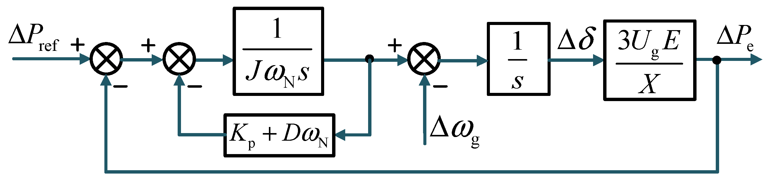
2. VSG Control Principle and Performance Analysis

The overall architecture of the proposed VSG control system in this paper is shown in Figure 2, which consists of the main circuit topology and an improved VSG control loop. Here, U_dc represents the DC-side voltage, U_abc denotes the capacitor voltage, U_g stands for the grid voltage, i_abc refers to the inductor current, i_d and i_q are the d-axis and q-axis components of the inductor current, respectively, u_d and u_q represent the d-axis and q-axis components of the capacitor voltage, L and C indicate the filter inductance and filter capacitance, L_g is the grid-side inductance, Q_ref and Q_e denote the reference value and output value of reactive power, E₀ and E correspond to the rated voltage amplitude and output voltage amplitude, and K_q signifies the reactive droop coefficient. This study focuses on the optimization and improvement of the VSG active power control loop, while the parameter design of the reactive power control loop and the dual-loop voltage–current control will not be elaborated.

The rotor motion equation for VSG control is expressed as

$$Js(\mathsf{\omega }-{\mathsf{\omega }}_{\mathrm{N}})+D(\mathsf{\omega }-{\mathsf{\omega }}_{\mathrm{N}})={\displaystyle \frac{P_{\mathrm{ref}}+K_{\mathrm{p}}({\mathsf{\omega }}_{\mathrm{N}}-\mathsf{\omega })-P_{\mathrm{e}}}{{\mathsf{\omega }}_{\mathrm{N}}}}$$

(1)

where P_ref and P_e represent the reference and output values of the active power, respectively, J denotes the moment of inertia, D is the damping coefficient, ω and ω_N correspond to the system output angular velocity and rated angular velocity, while K_p signifies the active power droop coefficient. According to the principle of line power transmission, the active power output of the grid-connected inverter is

$$P_{\mathrm{e}}={\displaystyle \frac{3U_{\mathrm{o}}{U}_{\mathrm{g}}\delta }{X}}={\displaystyle \frac{3U_{\mathrm{o}}{U}_{\mathrm{g}}}{X}}(\mathsf{\omega }-{\mathsf{\omega }}_{\mathrm{g}})$$

(2)

where X is the equivalent line impedance (X = ωL_g), δ denotes the phase difference between the VSG output voltage and the grid voltage, and ω_g represents the grid angular frequency. Neglecting the influence of the voltage and current inner loops, the small-signal block diagram of the P-f closed-loop system is derived as shown in Figure 3.

From Figure 3, the small-signal closed-loop transfer function of the P-f loop can be derived as

$$\Delta P_{\mathrm{e}}=G_{\mathrm{p}}(s)\Delta P_{\mathrm{ref}}+G_{\omega }(s)\Delta {\mathsf{\omega }}_{\mathrm{g}}$$

(3)

In Equation (3), G_p(s) and G_ω(s) represent the effects of the active power reference variation and grid frequency disturbance on the output power, respectively, with their expressions given as

$$\left\{\begin{array}{l}{G}_{\mathrm{p}}(s)={\displaystyle \frac{K}{J{\mathsf{\omega }}_{\mathrm{N}}{s}^2+(D{\mathsf{\omega }}_{\mathrm{N}}+K_{\mathrm{p}})s+K}}\\ G_{\omega }(s)={\displaystyle \frac{-K(J{\mathsf{\omega }}_{\mathrm{N}}s+D{\mathsf{\omega }}_{\mathrm{N}}+K_{\mathrm{p}})}{J{\mathsf{\omega }}_{\mathrm{N}}{s}^2+(D{\mathsf{\omega }}_{\mathrm{N}}+K_{\mathrm{p}})s+K}}\end{array}\right.$$

(4)

where K is the synchronization coefficient, given by K = 3U_oU_g/X.

Figure 4 shows the eigenvalue loci of the VSG active power control loop. With fixed J, increasing D converts a pair of complex conjugate poles into two negative real poles, transitioning the system from an underdamped to an overdamped state, thereby effectively suppressing power oscillations. Conversely, as J increases, the conjugate poles shift toward the imaginary axis, potentially inducing low-frequency oscillations.

When grid frequency fluctuations occur, the VSG control system performs primary frequency regulation, resulting in a steady-state error in the active power output given by

$$\Delta P_{\mathrm{e}}=\underset{s\to 0}{\lim }{G}_{\omega }(s)\Delta {\mathsf{\omega }}_{\mathrm{g}}=-(D{\mathsf{\omega }}_{\mathrm{N}}+K_{\mathrm{p}})\Delta {\mathsf{\omega }}_{\mathrm{g}}$$

(5)

As seen from Equation (5), increasing K_p or D will lead to a higher steady-state error. In practical engineering applications, a sufficiently large J must be selected to ensure adequate system inertia, making it challenging for the VSG control to simultaneously satisfy both dynamic and steady-state requirements.

3. Transient Damping Enhanced VSG Control

To address the challenge of coordinating dynamic and steady-state performance optimization in VSG control, this study introduces active-power low-frequency component feedback. This method provides an additional damping ratio without affecting the normal operation, thereby improving low-frequency stability.

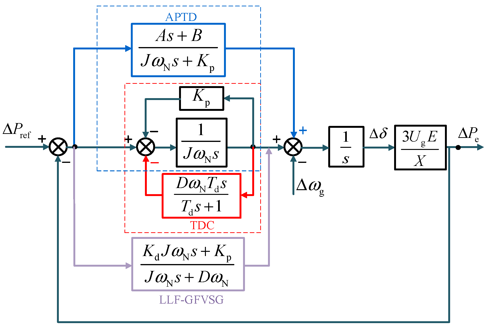
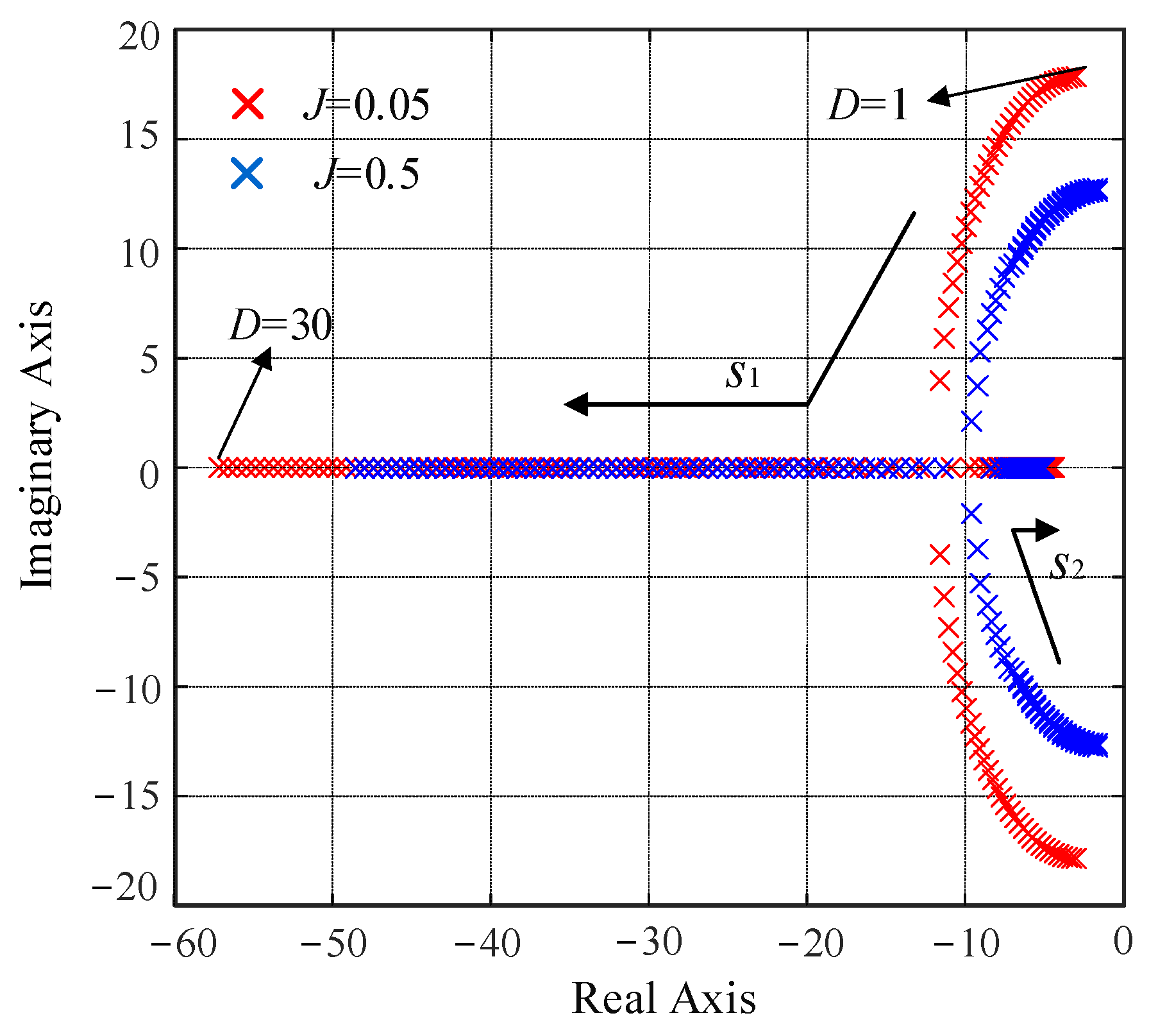
Transient Damping Enhancement Method and Stability Analysis

This paper enhances system damping during transients through active-power low-frequency component feedback, effectively suppressing power oscillations [18]. The corresponding control schematic is shown in Figure 5.

Based on Figure 5, the transient damping component can be converted into the time-domain representation and substituted into Equation (1) to obtain

$$J{\mathsf{\omega }}_{\mathrm{N}}{\displaystyle \frac{\mathrm{d}\mathsf{\omega }}{\mathrm{d}t}}=P_{\mathrm{ref}}-P_{\mathrm{e}}-(K_{\mathrm{p}}+D{\mathsf{\omega }}_{\mathrm{N}})\Delta \mathsf{\omega }-h_1\left[P_{\mathrm{e}}-h_2{\displaystyle {\int }_0^t{e}^{-h_2(t-\tau )}}{P}_{\mathrm{e}}(\tau )\mathrm{d}\tau \right]$$

(6)

Equation (6) indicates that the transient damping component introduces no feedback under steady-state conditions. During transients, its integral term rapidly decays without affecting the system state. Thus, the system state–space equation can be derived as

$$\left[\begin{array}{c}\Delta \ddot{\mathsf{\omega }}\\ \Delta {\ddot{P}}_{\mathrm{e}}\end{array}\right]=\left[\begin{array}{cc}-{\displaystyle \frac{K_{\mathrm{p}}+D{\mathsf{\omega }}_{\mathrm{N}}}{J{\mathsf{\omega }}_{\mathrm{N}}}}& -{\displaystyle \frac{h_1+1}{J{\mathsf{\omega }}_{\mathrm{N}}}}\\ 0& 0\end{array}\right]\left[\begin{array}{c}\Delta \dot{\mathsf{\omega }}\\ \Delta {\dot{P}}_{\mathrm{e}}\end{array}\right]+\left[\begin{array}{cc}0& {\displaystyle \frac{1}{J{\mathsf{\omega }}_{\mathrm{N}}}}\\ 1& 0\end{array}\right]\left[\begin{array}{c}\Delta {\ddot{P}}_{\mathrm{e}}\\ \Delta {\dot{P}}_{\mathrm{ref}}\end{array}\right]$$

(7)

The coefficient matrix in Equation (7) demonstrates that the feedback gain h₁ directly increases the system’s equivalent damping ratio, effectively suppressing the power oscillations. From Figure 5, the small-signal closed-loop transfer function of the transient damping-enhanced VSG active power loop is derived as

$$\Delta P_{\mathrm{e}}={G^{\prime }}_{\mathrm{p}}(s)\Delta P_{\mathrm{ref}}+{G^{\prime }}_{\omega }(s)\Delta {\mathsf{\omega }}_{\mathrm{g}}={\displaystyle \frac{K(s+h_2)}{J{\mathsf{\omega }}_{\mathrm{N}}{s}^3+C_1{s}^2+C_{2}s+K{h}_2}}\Delta P_{\mathrm{ref}}+{\displaystyle \frac{-JK{\mathsf{\omega }}_{\mathrm{N}}{s}^2-C_{1}Ks-K{K}_{\mathrm{p}}{h}_2-D{\mathsf{\omega }}_{\mathrm{N}}K{h}_2}{J{\mathsf{\omega }}_{\mathrm{N}}{s}^3+C_1{s}^2+C_{2}s+K{h}_2}}\Delta {\mathsf{\omega }}_{\mathrm{g}}$$

(8)

where C₁ and C₂ are

$$\left\{\begin{array}{c}{C}_1=J{\mathsf{\omega }}_{\mathrm{N}}{h}_2+K_{\mathrm{p}}+D{\mathsf{\omega }}_{\mathrm{N}}\\ C_2=D{\mathsf{\omega }}_{\mathrm{N}}{h}_2+h_2{K}_{\mathrm{p}}+h_{1}K+K\end{array}\right.$$

(9)

Comparing Equations (4) and (8), the TDF-VSG control introduces an additional pole-zero pair, which can be properly configured to cooperatively enhance both the dynamic performance and steady-state characteristics of the system.

Figure 6 shows the root locus of the TDF-VSG control system. The analysis reveals that: (a) when h₁ = 10, the complex conjugate poles s₁ and s₂ transition into two negative real roots as h₂ increases, exhibiting overdamped system characteristics, and (b) with h₂ = 80, increasing h₁ enhances the system damping ratio, but also drives pole s₃ closer to the imaginary axis, compromising the stability. To ensure optimal dynamic and steady-state performance after incorporating the transient damping component, the parameters are selected as h₁ = 10 and h₂ = 80.

Figure 7 compares the frequency-domain characteristics of VSG and TDF-VSG. Both transfer functions ΔP_e/ΔP_ref and ΔP_e/Δω_g demonstrate that TDF-VSG significantly improves the magnitude attenuation and phase margin in the low-frequency range of 0.1–10 Hz, thereby enhancing transient active power oscillation suppression. In conclusion, TDF-VSG effectively mitigates power oscillations while maintaining the system’s steady-state performance.

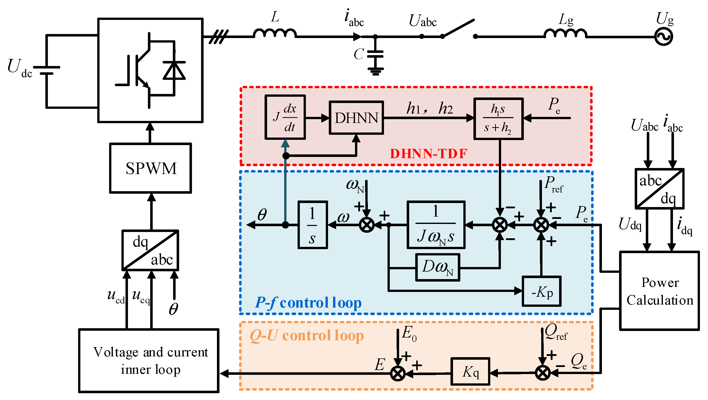
4. Dissipative Hamiltonian Neural Network-Based TDF-VSG Control Strategy

Under different disturbances, the optimal damping required by the system may vary. Fixed transient damping parameters h₁ and h₂ cannot achieve an optimal adjustment in such cases. Therefore, adaptive parameter tuning is necessary to simplify the design process and enhance the system robustness [19].

The Dissipative Hamiltonian Neural Network (DHNN) is a deep learning architecture that embeds Hamiltonian mechanics principles to decompose system dynamics into conservative and dissipative components. This hybrid approach combines neural networks’ universal approximation capability with the physical interpretability of Hamiltonian systems, enabling three key functions: data-driven Hamiltonian learning, a physics-constrained dynamic simulation, and nonlinear system identification with guaranteed convergence. As demonstrated in Figure 8, the customized DHNN implementation for TDF-VSG control delivers coordinated an improvement in both the transient response and steady-state regulation under complex grid conditions [20,21,22].

During system operation, the DHNN can emulate the physical characteristics of a synchronous generator, ensuring that the neural network’s output parameters comply with system operational constraints and energy conservation principles. The rotor motion equation of a synchronous generator during transient processes is represented by a second-order model, expressed as

$$\left\{\begin{array}{c}{\displaystyle \frac{\mathrm{d}\delta }{\mathrm{d}t}}={\mathsf{\omega }}_{\mathrm{N}}(\mathsf{\omega }-1)\\ T_{\mathrm{J}}{\displaystyle \frac{\mathrm{d}\mathsf{\omega }}{\mathrm{d}t}}=P_{\mathrm{m}}-P_{\mathrm{e}}-D(\mathsf{\omega }-1)\end{array}\right.$$

(10)

where T_J is the inertia time constant and P_m represents the input mechanical power of the generator. The units of ω_N and T_J are rad/s and s, respectively, while all other variables are expressed in per-unit values.

Based on the transient energy function construction method, multiplying both sides of the second equation in Equation (10) by dδ and substituting the first equation yields

$$T_{\mathrm{J}}{\mathsf{\omega }}_{\mathrm{N}}(\mathsf{\omega }-1)\mathrm{d}\mathsf{\omega }+P_{\mathrm{e}}\mathrm{d}\delta -P_{\mathrm{m}}\mathrm{d}\delta +D{\mathsf{\omega }}_{\mathrm{N}}{(\mathsf{\omega }-1)}^2\mathrm{d}t=0$$

(11)

By integrating both sides of Equation (11) and rearranging the terms, the transient energy balance equation of the synchronous generator can be derived as

$${\displaystyle \frac{1}{2}}{T}_{\mathrm{J}}{\mathsf{\omega }}_{\mathrm{N}}{(\mathsf{\omega }-1)}^2+{\displaystyle {\int }_{{\delta }_{\mathrm{N}}}^{\delta }{P}_{\mathrm{e}}\mathrm{d}\delta }-{\displaystyle {\int }_{{\delta }_{\mathrm{N}}}^{\delta }{P}_{\mathrm{m}}\mathrm{d}\delta }+{\displaystyle {\int }_0^{t}D{\mathsf{\omega }}_{\mathrm{N}}{(\mathsf{\omega }-1)}^2\mathrm{d}t=0}$$

(12)

where δ_N represents the power angle at the stable equilibrium point of the generator.

As seen from Equation (12), the energy during synchronous generator transients consists of three components: kinetic energy, potential energy, and dissipated energy. The first term on the left-hand side of the equation represents the generator’s kinetic energy, determined by ω; the second and third terms denote the potential energy generated by the combined action of the electromagnetic torque and mechanical torque after a disturbance, which depends on the initial and final states of the power angle; and the fourth term corresponds to the energy dissipated by generator damping.

Within the classical mechanics framework, the Hamiltonian H(p, q) is equivalent to the sum of a physical system’s kinetic and potential energies, typically expressed as

$$H(p,q)={\displaystyle \frac{1}{2}}{p}^{\mathrm{T}}{M}^{-1}(q)p+V(q)$$

(13)

where p represents the generalized momentum of the system, q denotes the generalized coordinates, and M(q) is the effective inertia matrix of the system. The term p^TM⁻¹(q)p/2 characterizes the kinetic energy of the system, while V(q) corresponds to the potential energy.

When the DHNN inputs p and q are Jω and θ, respectively, p^TM⁻¹(q)p/2 satisfies the kinetic energy constraints of a synchronous generator. The potential energy term for the rotational motion of the generator rotor can be expressed as

$$V(q)=T_{\mathrm{m}}-T_{\mathrm{e}}=J{\displaystyle \frac{\mathrm{d}\mathsf{\omega }}{\mathrm{d}t}}=J\ddot{q}$$

(14)

In Equation (14), T_m represents the mechanical torque output by the prime mover and T_e denotes the electromagnetic torque output of the generator.

The dissipation function D(p, q) is employed to model the dissipative term of the synchronous generator caused by factors such as friction and electromagnetic damping, defined as

$$D(p,q)={\displaystyle \frac{1}{2}}\left[\begin{array}{cc}p& q\end{array}\right]R(x)\left[\begin{array}{c}p\\ q\end{array}\right]={\displaystyle \frac{1}{2}}\left[\begin{array}{cc}p& q\end{array}\right]\left[\begin{array}{cc}{h}_1+D& 0\\ 0& h_2\end{array}\right]\left[\begin{array}{c}p\\ q\end{array}\right]$$

(15)

where the dissipation function consists of two parts: the damping loss related to the system’s angular velocity and the additional control loss related to the angle. As analyzed earlier, the transient damping parameters h₁ and h₂ are non-negative, so the matrix R(x) is a symmetric positive semi-definite matrix.

The above analysis has explained the physical meaning contained in the DHNN. Next, the control process of the DHNN is described. The output of the input layer of the DHNN is

$$O_j^{(1)}(k)=I^{(1)}(j),j=1,2$$

(16)

where I(k) denotes the input function, while O_j(k) represents the output function. Here, j, i, and l indicate the neuron counts in the input layer, hidden layer, and output layer, respectively, where the superscripts (1), (2), and (3) correspond to the input layer, hidden layer, and output layer.

The hidden layer input is

$$\left\{\begin{array}{c}{I}_{\mathrm{H}i}^{(2)}(k)=[I^{(1)}(1),I^{(1)}(2)]\\ I_{\mathrm{D}i}^{(2)}(k)=[I^{(1)}(1),I^{(1)}(2)]\end{array}\right.,i=1,\cdot \cdot \cdot ,4$$

(17)

The output of the hidden layer is

$$\left\{\begin{array}{c}{O}_{\mathrm{H}i}^{(2)}(k)=g_{\mathrm{H}}(I_{\mathrm{H}i}^{(2)}(k))\\ O_{\mathrm{D}i}^{(2)}(k)=g_{\mathrm{D}}(I_{\mathrm{D}i}^{(2)}(k))\end{array}\right.,i=1,\cdot \cdot \cdot ,4$$

(18)

In Equation (18), to ensure the non-negativity of the dissipation function, g_D(x) serves as a rectification function, defined as

$$g_{\mathrm{D}}(x)=\max (0,x)=\left\{\begin{array}{c}x,x\ge 0\\ 0,x<0\end{array}\right.$$

(19)

Meanwhile, the sub-network Net_H employs the Tanh function as g_H(x), since its origin symmetry and smooth gradient variations inherently preserve the energy conservation properties of Hamiltonian physical models. The expression for g_H(x) is

$$g_{\mathrm{H}}(x)=\tanh (x)={\displaystyle \frac{e^x-e^{-x}}{e^x+e^{-x}}}$$

(20)

The input to the output layer is

$$\left\{\begin{array}{c}{I}_{\mathrm{H}}^{(3)}(k)={\displaystyle \sum _{i=1}^4{w}_{\mathrm{H}i}{O}_{\mathrm{H}i}^{(2)}(k)}\\ I_{\mathrm{D}}^{(3)}(k)={\displaystyle \sum _{i=1}^4{w}_{\mathrm{D}i}{O}_{\mathrm{D}i}^{(2)}(k)}\end{array}\right.$$

(21)

In Equation (21), w_Hi and w_Di represent the weights connecting the hidden layer to the output layer. The output of the output layer is

$$\left\{\begin{array}{c}H(p,q)=O_{\mathrm{H}}^{(3)}(k)=f[I_{\mathrm{H}}^{(3)}(k)]\\ D(p,q)=O_{\mathrm{D}}^{(3)}(k)=f[I_{\mathrm{D}}^{(3)}(k)]\end{array}\right.$$

(22)

The output layer employs the sigmoid activation function, defined as

$$f(x)={\displaystyle \frac{u{e}^x}{e^x+e^{-x}}}$$

(23)

where u represents the upper bound of the output parameters.

After obtaining the dissipation function through Equation (22), the transient damping parameters are derived via a dissipation gradient calculation

$$h_1={\displaystyle \frac{{\partial }^{2}D(p,q)}{\partial p^2}}-D,h_2={\displaystyle \frac{{\partial }^{2}D(p,q)}{\partial q^2}}$$

(24)

To determine whether the DHNN requires weight updates, the errors between input gradients and target gradients are computed using H(p, q) and D(p, q), introducing an evaluation function defined as

$$L_{\mathrm{DHNN}}(k)={‖\left({\displaystyle \frac{\partial H(p,q)}{\partial p}}+{\displaystyle \frac{\partial D(p,q)}{\partial q}}\right)-\dot{q}‖}_2+{‖\left(-{\displaystyle \frac{\partial H(p,q)}{\partial q}}+{\displaystyle \frac{\partial D(p,q)}{\partial p}}\right)-\dot{p}‖}_2$$

(25)

To ensure H(p, q) and D(p, q) adhere to the physical laws of Hamiltonian mechanics, weight updates are triggered when the evaluation function is non-zero. This study employs a gradient descent for the weight adjustment, with the addition of an inertia term to accelerate algorithm convergence.

$$\left\{\begin{array}{c}\Delta w_{\mathrm{H}i}^{(3)}(k)=-\eta {\displaystyle \frac{\partial L_{\mathrm{DHNN}}(k)}{\partial w_{\mathrm{H}i}^{(3)}}}+\alpha \Delta w_{\mathrm{H}i}^{(3)}(k-1)\\ \Delta w_{\mathrm{D}i}^{(3)}(k)=-\eta {\displaystyle \frac{\partial L_{\mathrm{DHNN}}(k)}{\partial w_{\mathrm{D}i}^{(3)}}}+\alpha \Delta w_{\mathrm{D}i}^{(3)}(k-1)\end{array}\right.$$

(26)

where η denotes the learning rate and α represents the momentum coefficient. The parameter selection criteria are detailed in Appendix A.

The control steps based on the DHNN algorithm are as follows:

(1)

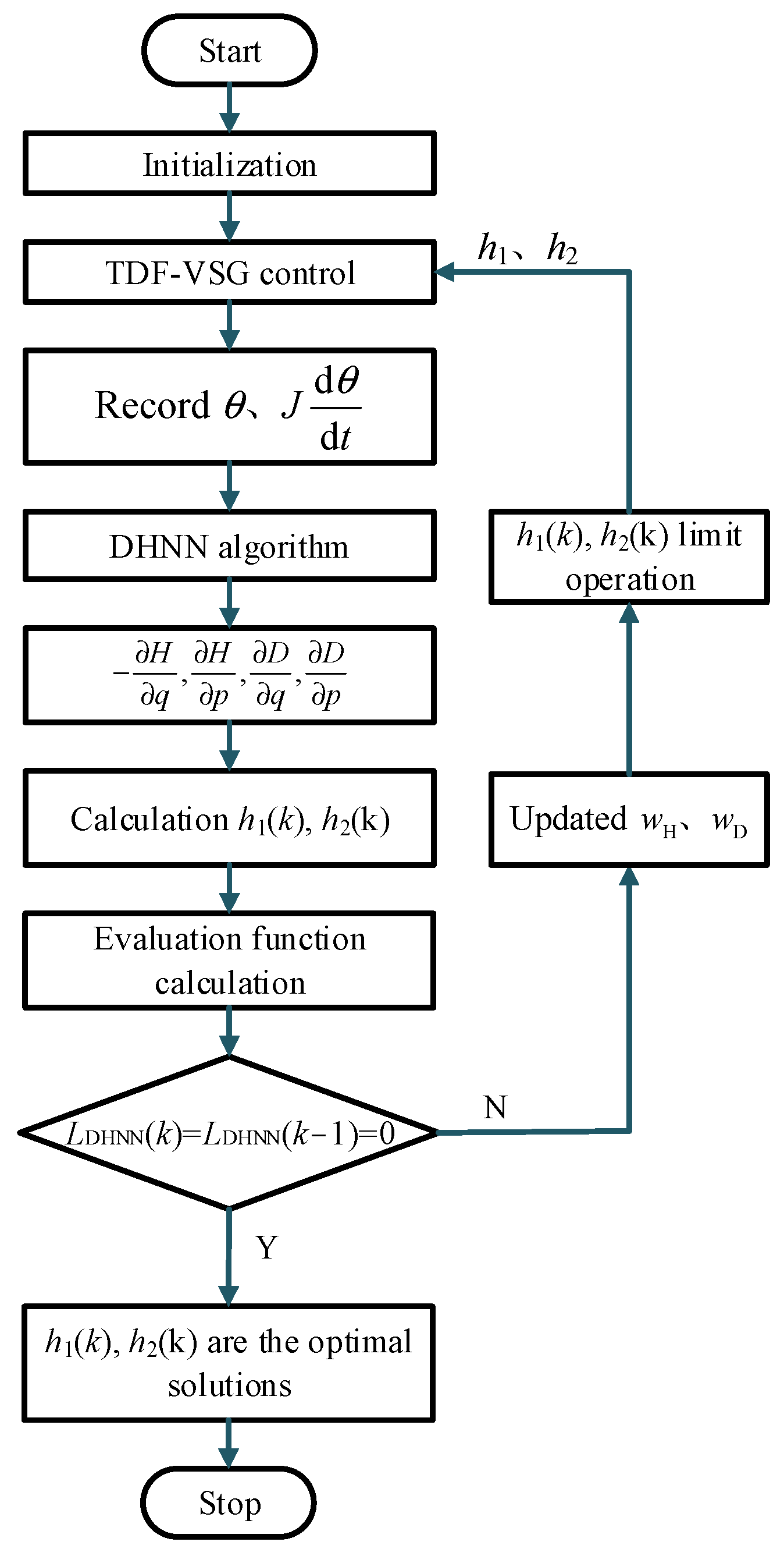
Parameter Initialization: The algorithm requires setting the initial transient damping parameters h₁, h₂ and the initial weights w_H, w_D. This study employs the Xavier initialization method, where weights are initialized as normally distributed signals with a mean of 0 and variance of 2/(n_in + n_out). This ensures consistent variance in the data during forward propagation and gradients during backpropagation in the early stages of network learning, thereby accelerating convergence and enhancing the stability. The weight initialization formula is given by

$$w~\mathcal{N}(0,{\displaystyle \frac{2}{n_{\mathrm{in}}+n_{\mathrm{out}}}})$$

(27)

In Equation (27), n_in and n_out represent the number of input and output neurons, respectively.

(2)

TDF-VSG Control: The transient damping parameters (either initial or real-time-adjusted) output by the DHNN are introduced into the TDF branch to improve the VSG control system. Meanwhile, the θ value from the VSG active power control loop is processed and fed into the DHNN.

(3)

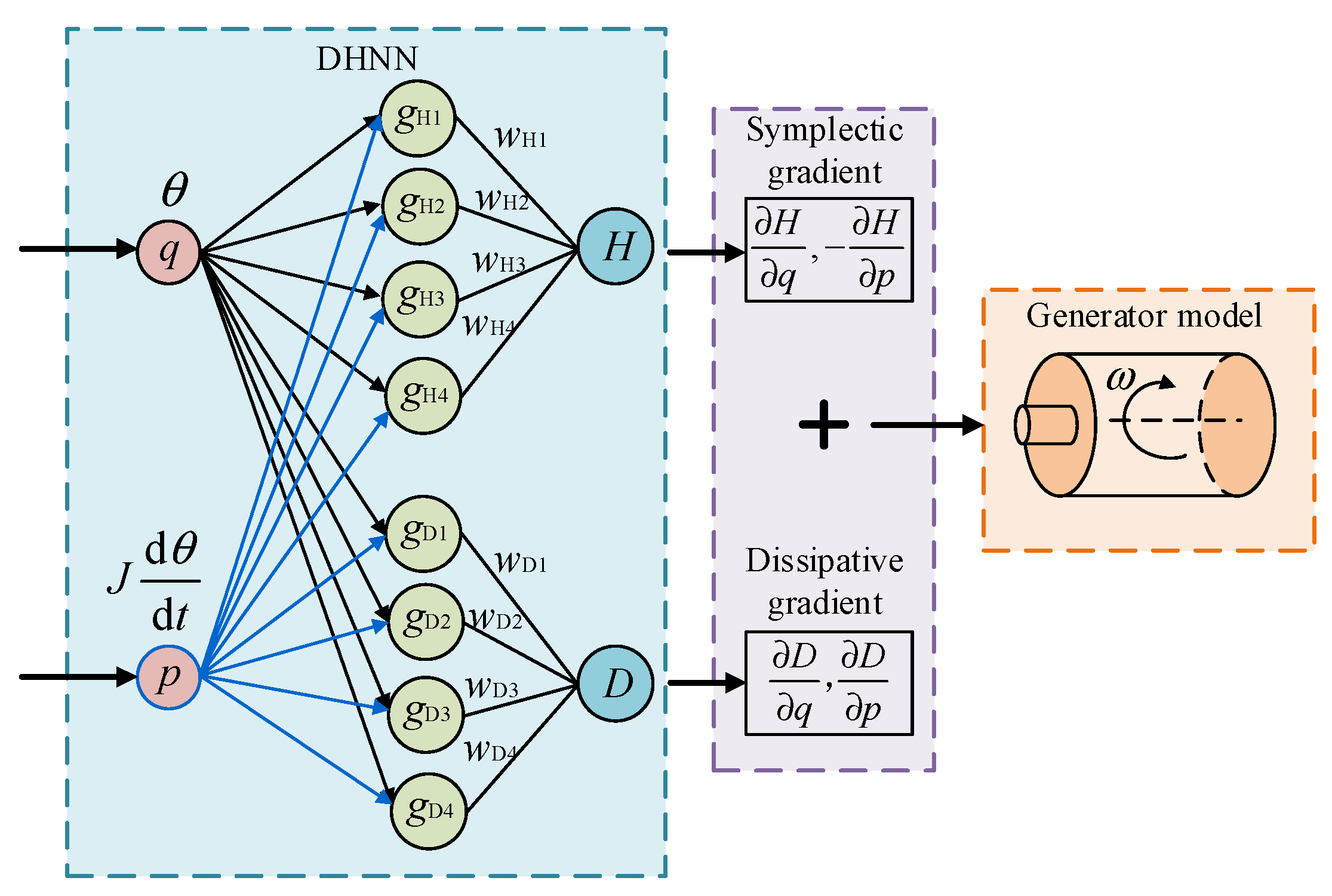
DHNN Forward Computation: the Hamiltonian H(p,q) and dissipation function D(p,q) are computed through Equations (16)–(22).

(4)

Dynamic Calculation of Transient Damping Parameters: based on the dissipation function obtained in step (3), the transient damping parameters h₁ and h₂ are calculated using Equation (24).

(5)

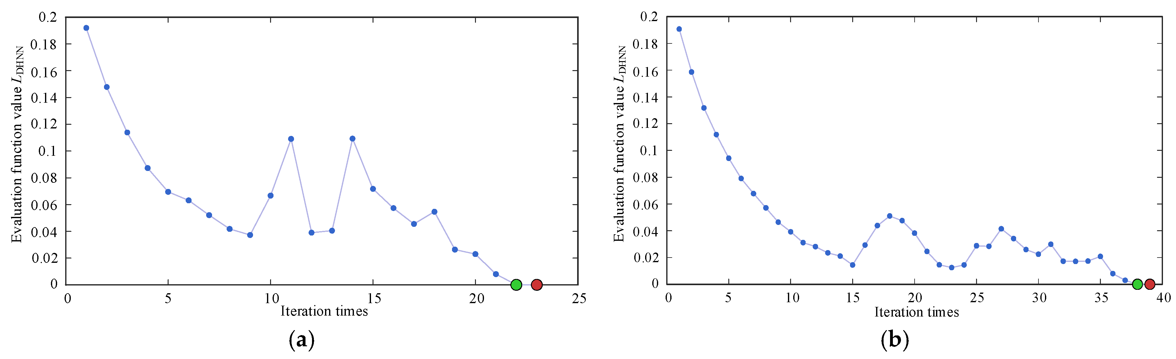
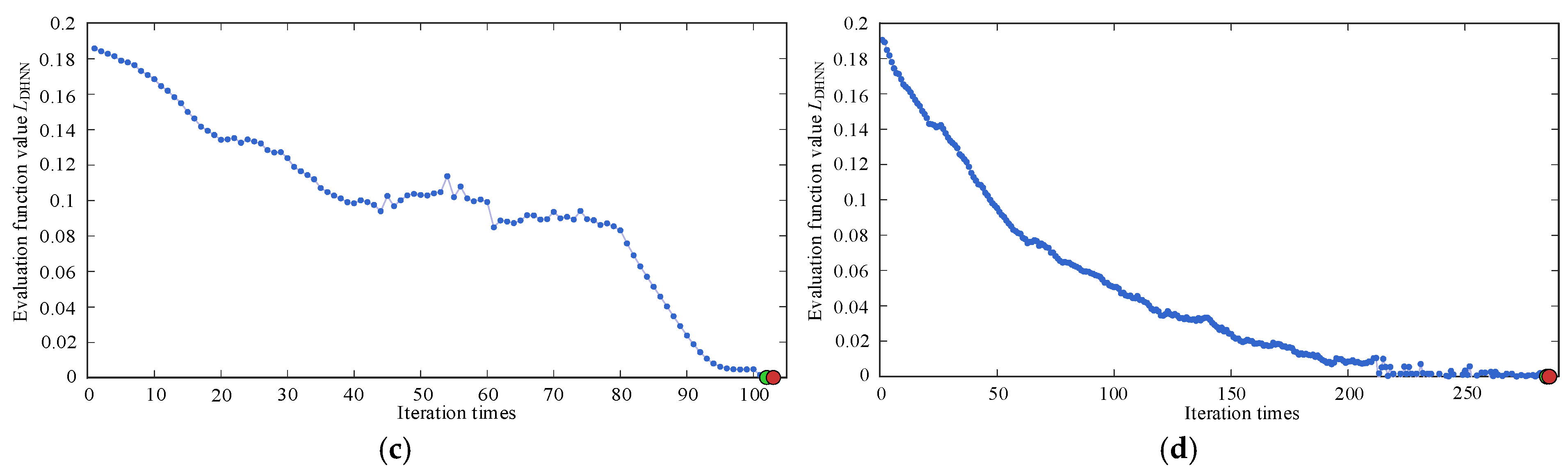
Evaluation Function Calculation and Weight Update: The evaluation function value for the current time step is computed using Equation (25). If the stopping criterion is not met (i.e., when the evaluation function values of both the current and previous iterations are not equal to zero), the weights are updated using Equation (26). The transient damping parameters h₁ and h₂ obtained in step (4) are then output to the TDF-VSG control loop to complete the closed-loop control.

(6)

Algorithm Termination and Triggering: The parameter optimization process terminates when the evaluation function meets the stopping criterion, at which point the transient damping parameters represent the optimal solution. The DHNN training process is re-triggered when grid disturbances are detected by the system.

Figure 9 shows the flowchart of the DHNN-TDF-VSG control algorithm.

5. Simulation and Experimental Verification

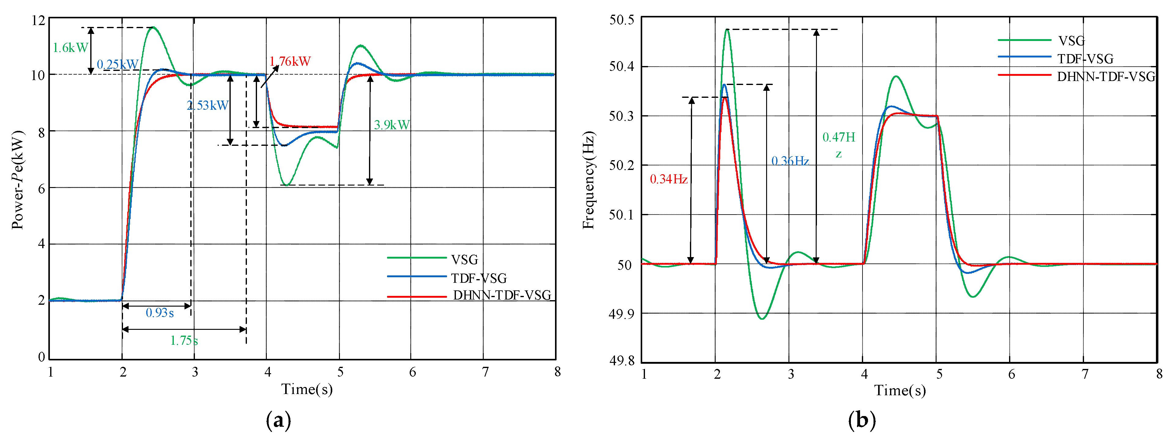
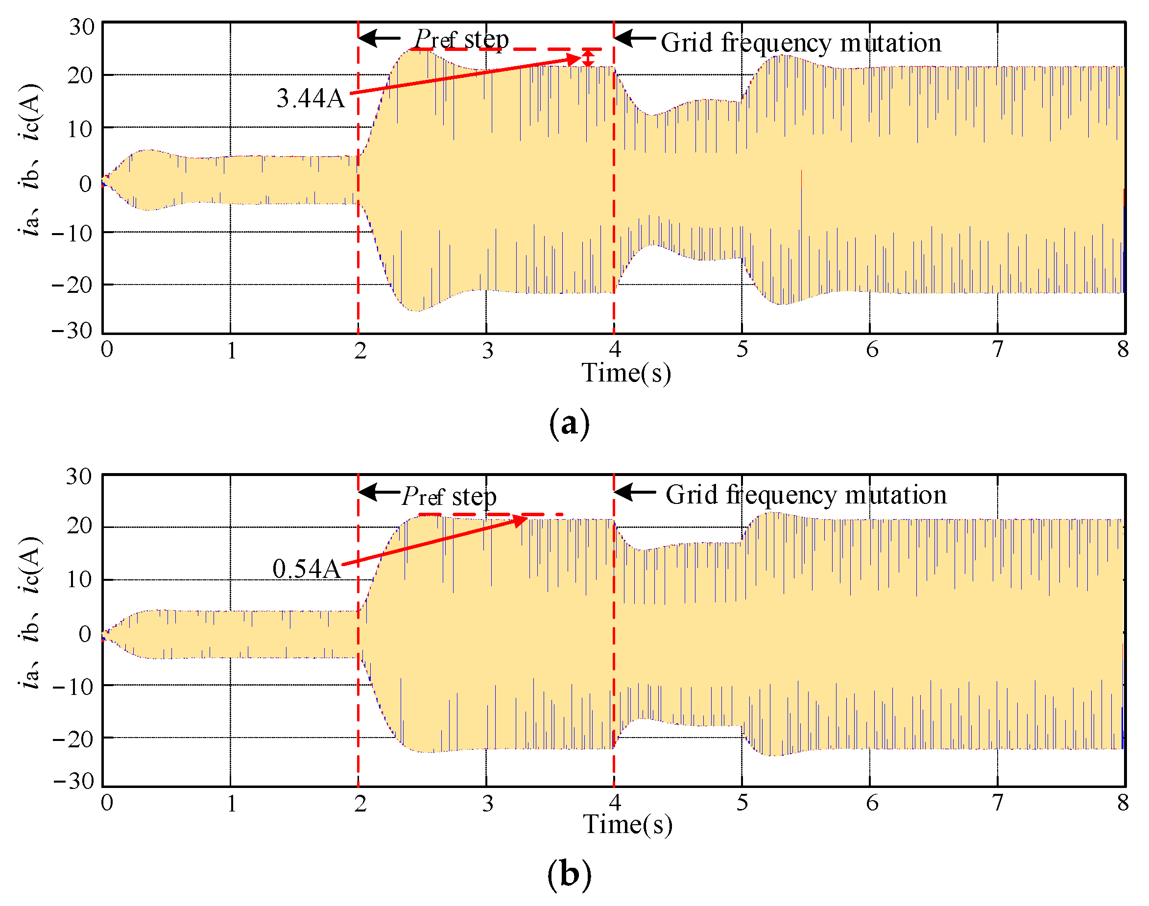
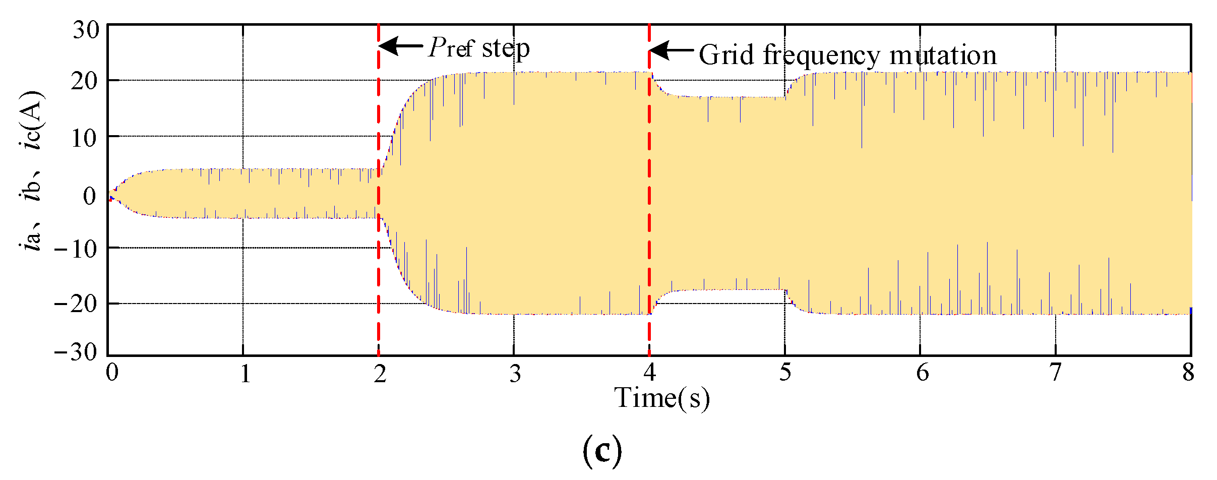
5.1. Comparative Analysis of Different Control Strategies Through Simulation

To validate the effectiveness of the proposed control strategy, a VSG grid-connected simulation model was developed in MATLAB/Simulink, as shown in Figure 2, with detailed parameters listed in

Table 1. Key system parameters.

Parameter	Numerical Value	Parameter	Numerical Value
Udc/V	800	J/(kg·m2)	0.1
Ug/V	380	Kp	200
E0/V	311	D/(N·m·s·rad−1)	15
ωN/(rad/s)	314	L/mH	3
Lg/mH	30	C/μF	10

. The simulation scenarios include (1) a step change in P_ref from 2 kW to 10 kW at t = 2 s; (2) a grid frequency surge to 50.3 Hz at t = 4 s; and (3) frequency recovery to 50 Hz at t = 5 s.

The key parameters of the dissipative Hamiltonian neural network adaptive control strategy are listed in

Table 2. Key parameters of the DHNN algorithm.

Parameter	Numerical Value	Parameter	Numerical Value
Learning rate η	0.08	Maximum h1	15
Inertial coefficient α	0.6	Minimum h1	7
Initial value h1	10	Maximum h2	100
Initial value h2	80	Minimum h2	70

.

To validate the effectiveness of the control strategy, this paper presents a comparative analysis of the active power response characteristics among VSG, TDF-VSG, and DHNN-TDF-VSG, with simulation results shown in Figure 10.

Figure 10 compares the active power response characteristics under three control strategies. The conventional VSG scheme exhibits oscillations during both P_ref step changes and ω_g disturbances, demonstrating a poor dynamic and steady-state performance. In contrast, the TDF-VSG solution reduces active power overshoot by 84.4%, decreases the settling time by 46.9%, and limits the steady-state error to 2.53 kW. The proposed DHNN-TDF-VSG control scheme further eliminates power oscillations while reducing the steady-state error to 1.76 kW. These results verify that the proposed strategy simultaneously improves the steady-state accuracy and suppresses transient active power oscillations.

Figure 11 compares the output current waveforms under the three control strategies. When employing DHNN-TDF-VSG control, the output current smoothly transitions to a steady state during both P_ref step changes and ω_g disturbances, with no oscillations or overshoot observed.

The adaptive curves of the transient damping parameters h₁ and h₂ output by the DHNN are shown in Figure 12. As observed from the figure, after sufficient learning iterations, the DHNN can rapidly determine optimal h₁ and h₂ parameters based on real-time system information when disturbances occur, thereby enhancing both the dynamic and steady-state performance. During stable operation intervals, the DHNN maintains system stability without unnecessary control actions.

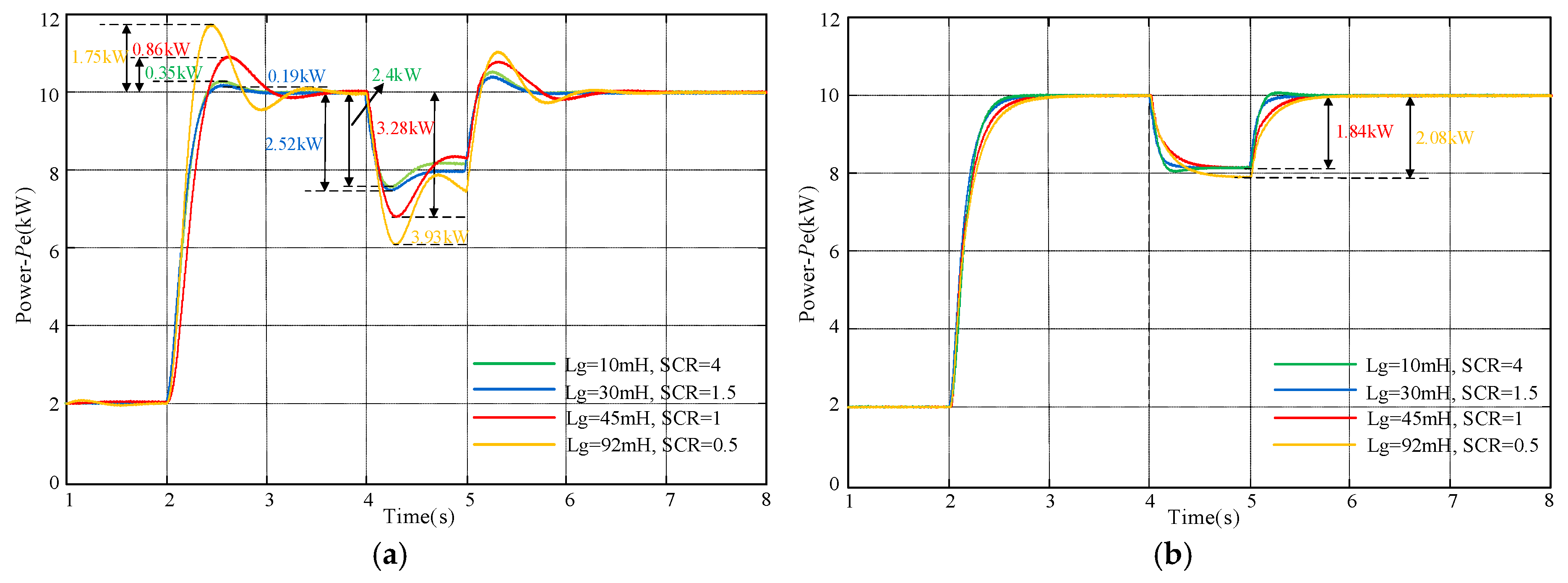
5.2. Comparative Robustness Analysis of Control Strategies Under Different Grid Strength Conditions

To verify the enhanced robustness of the proposed DHNN-TDF-VSG control strategy against grid strength variations compared to TDF-VSG, simulations were conducted under identical control parameters across different grid strength conditions. The results are presented in Figure 13.

Figure 13a presents simulation results of the TDF-VSG control strategy under different SCR conditions. When SCR = 4 and 1.5, the active power overshoots are 0.35 kW and 0.19 kW, respectively, with steady-state errors of 2.4 kW and 2.52 kW. For SCR = 1, the overshoot increases to 0.86 kW with a steady-state error of 3.28 kW. Under the extreme condition of SCR = 0.5, the overshoot and steady-state errors further escalate to 1.75 kW and 3.93 kW, respectively. These results demonstrate that the fixed-parameter TDF-VSG control exhibits poor adaptability to grid impedance variations, failing to effectively improve both the dynamic and steady-state performance.

As shown in Figure 13b, even under the extreme SCR = 0.5 condition, the proposed strategy effectively suppresses low-frequency power oscillations, with only a 0.24 kW increase in the steady-state error compared to the other three SCR cases. This verifies that the DHNN-TDF-VSG control strategy can successfully mitigate active power oscillations across various grid strengths, demonstrating superior robustness.

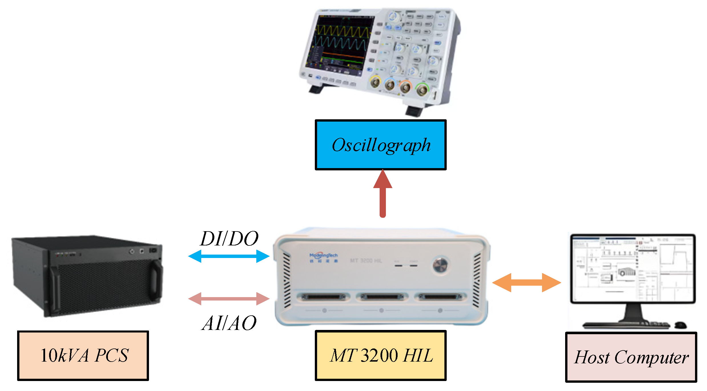
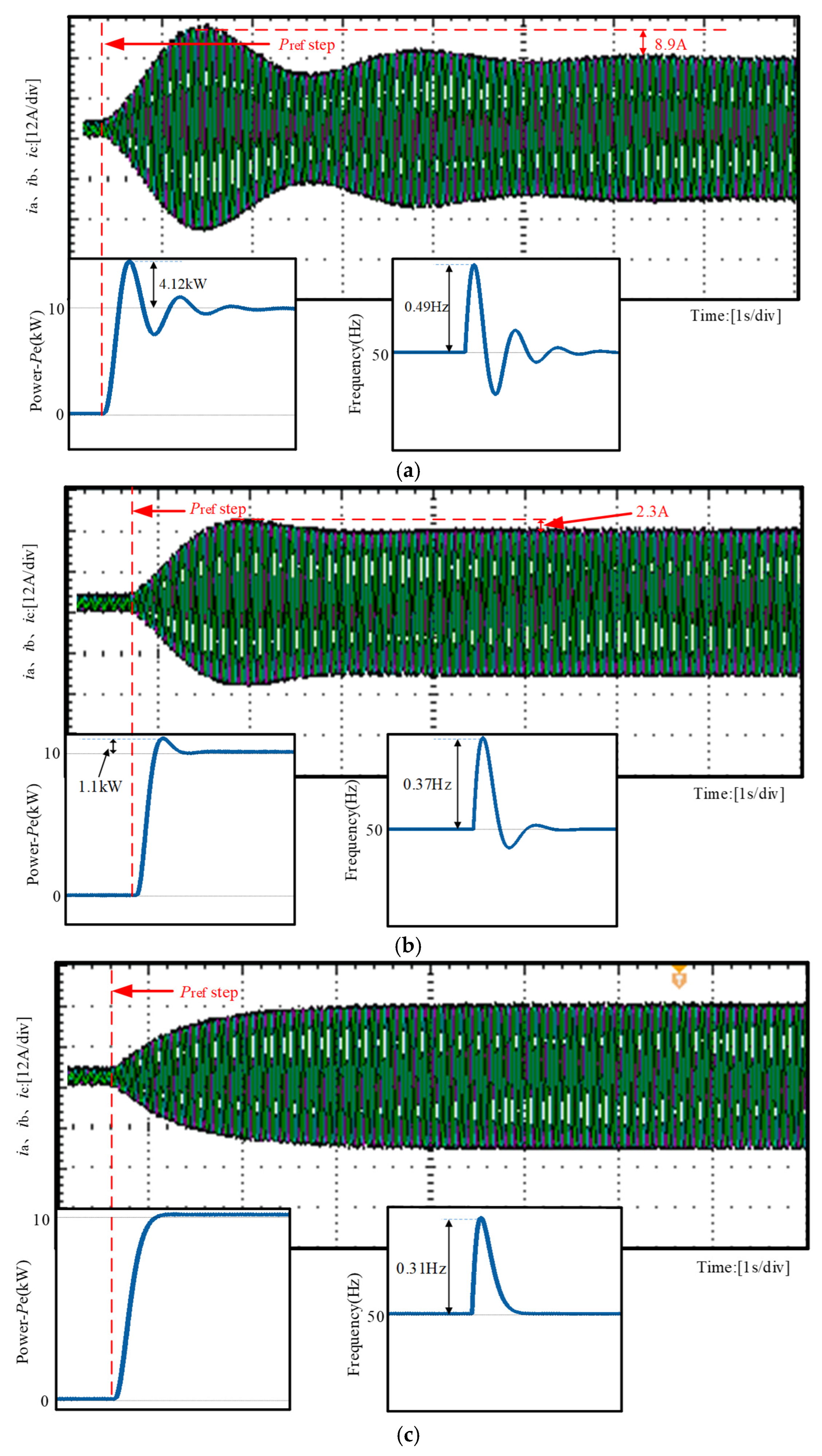
5.3. Comparative Analysis of Experiments Under Different Control Strategies

To further validate the effectiveness of the proposed control strategy, comparative experiments were conducted on a hardware-in-the-loop (HIL) platform, as shown in Figure 14. The test scenario was configured with an active power reference step change from 0 kW to 10 kW. The system’s active power oscillations and frequency fluctuations under different control strategies were monitored via the host computer, while output current waveforms were captured and analyzed using an oscilloscope for a comparative evaluation.

Figure 15 shows the comparison of the output active power, frequency, and output current waveforms under different control strategies when P_ref undergoes a step change. It can be observed from the figure that the experimental results are consistent with the simulation results under the condition of an active power reference step change. Compared with the VSG control, the TDF-VSG control strategy can effectively suppress transient power oscillations and frequency fluctuations, reducing the overshoot of the output current by 5.3 A. Furthermore, the DHNN-TDF-VSG control strategy further suppresses low-frequency oscillations on this basis, with no overshoot in the output active power, thereby verifying the effectiveness of the proposed control strategy in this paper.

6. Conclusions

This paper presents an adaptive transient damping VSG control strategy based on the dissipative Hamiltonian neural network (DHNN). By incorporating a transient damping feedback control loop into the conventional VSG control framework, the proposed strategy effectively reduces the steady-state error while significantly suppressing low-frequency oscillations in the system. Compared with traditional VSG control, the proposed TDF-VSG strategy reduces the active power overshoot by 84.4%, regulation time by 46.9%, and steady-state error by 35.1% when the short-circuit ratio (SCR) is 1.5. Building on this, the dissipative Hamiltonian neural network, based on the dissipative Hamiltonian equation, is introduced to further optimize the transient damping parameters. Compared with the TDF-VSG strategy, the proposed DHNN-TDF-VSG strategy further suppresses active power oscillations and reduces the steady-state error to 30.4% when SCR is 1.5. The verification results under different grid strengths show that the DHNN-TDF-VSG control strategy can effectively reduce active power overshoot. In summary, the proposed strategy has a good dynamic performance and robustness, providing a new idea and method for the optimization of VSG control strategies.

References

1. Xie, B.; Zheng, W.; Li, P.; Shi, Y.; Su, J. Stability analysis and admittance reshaping for PQ inverters with different power control methods. Int. J. Electr. Power Energy Syst. 2025, 166, 110541. [Google Scholar] [CrossRef]
2. Zheng, Y.; Han, Y.; Wang, C.; Ren, Q.; Yang, P.; Zalhaf, A.S. Impact of phase-locked loop on grid-connected inverter stability under weak grid conditions and suppression measures. Comput. Electr. Eng. 2025, 123, 110249. [Google Scholar] [CrossRef]
3. Su, Z.; Yang, G.; Yao, L. Transient Frequency Modeling and Characteristic Analysis of Virtual Synchronous Generator. Energies 2025, 18, 1098. [Google Scholar] [CrossRef]
4. Yin, J.; Chen, Z.; Qian, W.; Zhou, S. A Virtual Synchronous Generator Low-Voltage Ride-Through Control Strategy Considering Complex Grid Faults. Appl. Sci. 2025, 15, 1920. [Google Scholar] [CrossRef]
5. Mousavi, H.M.; Moradi, H. Simultaneous compensation of distorted DC bus and AC side voltage using enhanced virtual synchronous generator in Islanded DC microgrid. Int. J. Electron. 2025, 112, 151–176. [Google Scholar] [CrossRef]
6. Shi, R.; Lan, C.; Dong, Z.; Yang, G. An Active Power Dynamic Oscillation Damping Method for the Grid-Forming Virtual Synchronous Generator Based on Energy Reshaping Mechanism. Energies 2023, 16, 7723. [Google Scholar] [CrossRef]
7. Mehdi, P.; Mohammadreza, T. Designing a central MIMO state feedback controller for a microgrid with multi-parallel VSGs to damp active power oscillations. Int. J. Electr. Power Energy Syst. 2021, 133, 106984. [Google Scholar]
8. Shuai, Z.; Huang, W.; Shen, Z.J.; Luo, A.; Tian, Z. Active Power Oscillation and Suppression Techniques Between Two Parallel Synchronverters During Load Fluctuations. IEEE Trans. Power Electron. 2020, 35, 4127–4142. [Google Scholar] [CrossRef]
9. Xia, Y.; Wang, Y.; Chen, Y.; Shi, J.; Yang, Y.; Li, W.; Li, K. A Cooperative Adaptive VSG Control Strategy Based on Virtual Inertia and Damping for Photovoltaic Storage System. Energies 2025, 18, 1505. [Google Scholar] [CrossRef]
10. Soni, N.; Doolla, S.; Chandorkar, M.C. Improvement of Transient Response in Microgrids Using Virtual Inertia. IEEE Trans. Power Deliv. 2013, 28, 1830–1838. [Google Scholar] [CrossRef]
11. Ashabani, M.; Mohamed, Y.A.R.I. Integrating VSCs to Weak Grids by Nonlinear Power Damping Controller with Self-Synchronization Capability. IEEE Trans. Power Syst. A Publ. Power Eng. Soc. 2014, 29, 805–814. [Google Scholar] [CrossRef]
12. Zhang, L.; Shi, R.; Li, J.; Yu, Y.; Zhang, Y. Improved Strategy of Grid-Forming Virtual Synchronous Generator Based on Transient Damping. Energy Eng. 2024, 121, 3181–3197. [Google Scholar] [CrossRef]
13. Shi, R.; Lan, C.; Huang, J.; Ju, C. Analysis and Optimization Strategy of Active Power Dynamic Response for VSG under a Weak Grid. Energies 2023, 16, 4593. [Google Scholar] [CrossRef]
14. Xia, Y.; Chen, Y.; Wang, Y.; Chen, R.; Li, K.; Shi, J.; Yang, Y. A Virtual Synchronous Generator Control Strategy Based on Transient Damping Compensation and Virtual Inertia Adaptation. Appl. Sci. 2025, 15, 728. [Google Scholar] [CrossRef]
15. Qian, J.; Xu, L.; Ren, X.; Wang, X. Structured Deep Neural Network-Based Backstepping Trajectory Tracking Control for Lagrangian Systems. IEEE Trans. Neural Netw. Learn. Systems 2024, 10, 1109. [Google Scholar] [CrossRef]
16. Marco, D.; Florian, M. Symplectic learning for Hamiltonian neural networks. J. Comput. Phys. 2023, 494, 112495. [Google Scholar]
17. Stegink, T.; Persis, D.C.; Schaft, D.V.A. Port-Hamiltonian Formulation of the Gradient Method Applied to Smart Grids. IFAC Pap. 2015, 48, 13–18. [Google Scholar] [CrossRef]
18. Yang, B.; Li, H.; Zhang, Y.; Lu, S. Grid frequency disturbance analysis based virtual synchronous generator transient performance improvement control. Int. J. Electr. Power Energy Syst. 2025, 166, 110572. [Google Scholar] [CrossRef]
19. Gurski, E.; Kuiava, R.; Perez, F.; Benedito, R.A.; Damm, G. A Novel VSG with Adaptive Virtual Inertia and Adaptive Damping Coefficient to Improve Transient Frequency Response of Microgrids. Energies 2024, 17, 4370. [Google Scholar] [CrossRef]
20. Cheng, X.; Wang, L.; Cao, Y. Quadrature Based Neural Network Learning of Stochastic Hamiltonian Systems. Mathematics 2024, 12, 2438. [Google Scholar] [CrossRef]
21. Liu, Y.; Li, J.; Ding, Q.; Chu, B. Dissipative Hamiltonian realisation and decentralised saturated control of multi-machine multi-load power systems. IET Control Theory Appl. 2013, 7, 1287–1293. [Google Scholar] [CrossRef]
22. Fan, B.; Huang, G.; Sun, L.; Zhao, Y.; Zhou, H.; Wang, J. Disturbance Rejection Control Method Based on Variable Damping and Port Controlled Hamiltonian with Dissipation Model for Induction Drive Motor. Int. J. Precis. Eng. Manuf. 2023, 24, 2009–2019. [Google Scholar] [CrossRef]
Figure 1. The proposed transient damping control block diagram.
Electronics 14 02207 g001
Figure 2. Main circuit and control block diagram of VSG.
Electronics 14 02207 g002
Figure 3. Small-signal model of the active power loop.
Electronics 14 02207 g003
Figure 4. Closed-loop root loci of the VSG active power control loop.
Electronics 14 02207 g004
Figure 5. Control diagram of the transient damping-enhanced VSG active power-frequency loop.
Electronics 14 02207 g005
Figure 6. Root locus of the TDF-VSG closed-loop control system: (a) h1 = 10 with h2 varying from 1 to 200. (b) h2 = 80 with h1 varying from 1 to 100.
Electronics 14 02207 g006
Figure 7. Frequency response comparison between VSG and TDF-VSG: (a) ΔPePref. (b) ΔPeωg.
Electronics 14 02207 g007
Figure 8. Architecture diagram of DHNN-TDF-VSG control system.
Electronics 14 02207 g008
Figure 9. Control flowchart of the DHNN algorithm.
Electronics 14 02207 g009
Figure 10. Active power response characteristics under different control strategies: (a) Pe comparison. (b) Frequency comparison.
Electronics 14 02207 g010
Figure 11. Output current under different control strategies: (a) VSG. (b) TDF-VSG. (c) DHNN-TDF-VSG.
Electronics 14 02207 g011aElectronics 14 02207 g011b
Figure 12. Adaptive transient damping parameters: (a) h1 curve. (b) h2 curve.
Electronics 14 02207 g012
Figure 13. Comparative results of control strategies under different SCR conditions: (a) TDF-VSG. (b) DHNN-TDF-VSG.
Electronics 14 02207 g013
Figure 14. Semi-physical experimental platform.
Electronics 14 02207 g014
Figure 15. Experimental results: (a) VSG. (b) TDF-VSG. (c) DHNN-TDF-VSG.
Electronics 14 02207 g015