Efficient Charging Pad Deployment in Large-Scale WRSNs: A Sink-Outward Strategy

Abstract

In recent years, a key problem in wireless sensor networks has been how to effectively deploy the minimum number of wireless charging pads while establishing at least one feasible charging path from the base station. This ensures that the unmanned aerial vehicle can reach and recharge all sensor nodes from the BS. Previous works have often employed greedy algorithms to solve the optimal deployment problem, treating coverage and connectivity as interdependent properties. This has led to excessive constraints on the placement of wireless charging pads, as each newly added charging pad has to satisfy both properties at the same time. Additionally, previous works have overlooked the critical issue of avoiding the occurrence of isolated sensor nodes in uncovered fragmented regions, in deployment. Failing to address this issue requires additional deployment costs to compensate for uncovered nodes. To overcome these limitations, in this work, we propose a sink-outward strategy wireless charging pad deployment algorithm, which deploys charging pads layer by layer from the innermost region outward, prioritizing coverage before connectivity. The proposed sink-outward max covering (SMC) consists of two key steps: initial pad deployment and optimization. The simulation results show that the proposed method SMC combined with the optimization step, called reducing pads by reallocating pads partially (RPRAP), achieves a reduction in pad count of 10.6–19.8% compared with the methods used in previous works, and the execution time demonstrated in previous works is several to tens of times longer than that of SMC combined with RPRAP. Moreover, the proposed redundant pad removal step, RPRAP, not only removes more redundant pads than the methods used in previous works but also drastically reduces processing time in large-scale wireless sensor networks with many redundant pads.

1. Introduction

Wireless sensor networks (WSNs) serve as a key technology in the Internet of Things (IoT) and have a wide range of applications, including military intelligence transmission, vehicle tracking and detection, healthcare assistance and monitoring, quality control, warehouse management, natural disaster warnings, and home applications [1]. Among these applications, energy plays a critical role in WSNs. This is primarily due to the small size of the sensors, which limits the capacity of the batteries they carry. Additionally, replacing batteries to extend the lifespan of a sensor is often impractical. Recent advancements in wireless charging technology have led researchers to explore wireless power transfer (WPT) as a new energy source for WSNs. As the efficiency of wireless charging has significantly improved (exceeding 82% for short-range charging) [2], WSNs equipped with rechargeable devices have emerged as a promising platform for future applications; such networks are referred to as wireless rechargeable sensor networks (WRSNs) [3]. Typically, WRSNs require the deployment of several wireless chargers. Compared with static wireless chargers, wireless charger vehicles (WCVs), which are chargers mounted on mobile platforms, have become a prominent research topic in recent years.

Moreover, unmanned aerial vehicles (UAVs) have been widely integrated into daily life. To overcome the limitations of UAV battery capacity, various wireless charging technologies for UAVs have been developed [4]. Building on this, researchers have proposed equipping UAVs with chargers, creating what are known as wireless charging drones (WCDs) [5,6] to provide real-time charging services for WRSNs. Another emerging development is the wireless charging pad (WCP) [5,7], which offers new wireless power charging technology for WCDs.

When designing optimization algorithms for WCP deployment, it is essential to consider connectivity, coverage, and geometric properties [5,7]. However, previous approaches have often used greedy algorithms, which typically address coverage and connectivity simultaneously, to solve WCP deployment optimization problems [5]. This approach overly restricts the placement of WCPs, such as deploying them only at sensor locations. Additionally, greedy algorithms tend to be overly conservative, leading to the deployment of excessive WCPs. Furthermore, prior studies have overlooked a critical issue: avoiding the deployment of WCPs in a way that leaves a small number of sensors stranded in uncovered fragmented areas, which can result in higher costs when attempting to address these gaps later.

To address these issues, this work proposes a novel algorithm for WCP deployment that starts from the sink and expands outward, prioritizing coverage before considering connectivity. By leveraging computational geometry techniques and properties, we aim to overcome the aforementioned limitations and provide a more effective solution to the WCP deployment problem. The proposed approach, called sink-outward max covering (SMC), consists of two key steps: initial pad deployment and optimization. A related study found that adding a redundant pad removal step reduces the number of pads required for configuration but may increase processing time [8]. However, simulation results demonstrate that the proposed SMC method combined with a new optimization step, called reducing pads by reallocating pads partially (RPRAP), achieves a reduction in pad count of 10.6–19.8% compared with the methods used in previous works. Additionally, the execution time demonstrated in previous works is several to tens of times longer than that of SMC combined with RPRAP. Furthermore, the optimization step, RPRAP, not only removes more redundant pads than the methods used in previous works but also significantly reduces processing time, especially when dealing with large-scale WSNs with numerous redundant pads.

The rest of this paper is organized as follows. Section 2 presents a survey of previous related works. Section 3 presents the proposed SMC for deploying charging pads. Section 4 describes the simulation results with discussions. Finally, Section 5 concludes this work.

2. Related Works

To grasp the related works on wireless charging, this section introduces related yet distinct outcomes and presents necessary discussion.

In [9], Y. Shu et al. explored how to continuously control the optimal moving speed of a mobile wireless charger on a fixed trajectory to reduce movement time while increasing charging time, thereby maximizing the minimum charging power in the entire network. When this problem involved multiple mobile wireless chargers, they demonstrated that it is NP-hard.

In [10], L. Fu et al. proposed the concept of constructing nested traveling salesman paths to prevent mobile wireless chargers from unnecessarily visiting well-powered sensors.

In [11], Cheng et al. introduced the use of a charging vehicle to replenish power for sensors and designed a distance-based nearest job first scheduling algorithm with a mechanism for predicting bottlenecks and random removal, deriving an upper bound for shorter paths.

In [2], M. Zhao et al. utilized a multifunctional mobile device to perform dual tasks of data collection and wireless charging. Their dual tasks consisted of two steps: the first step involved periodically selecting a portion of sensors as anchors for the mobile device to visit sequentially, providing unlimited charging and collecting information from the sensor network. The second step involved calculating the network usage maximization problem and proposing a distributed algorithm to adjust the data rate, link scheduling, and traffic routing for sensors sending buffered data to the mobile device while the device moved between anchors.

In [12], C. Wang et al. separated the tasks of data collection and wireless charging, assigning them to different types of mobile vehicles. Their proposed method considered group size and designed a mathematical model to calculate and estimate data collection time and the minimum number of mobile wireless chargers required.

In [13,14], L. Xie et al. transformed the power charging problem into a traveling salesman problem based on energy distribution and power consumption. Their formulated periodic charging scheme is divided into single-point and multi-point charging schemes. The single-point charging scheme involves one charging machine charging a single sensor point at a time, while the multi-point charging scheme allows simultaneous charging of multiple nearby sensor points to increase efficiency.

In [15], Guo et al. addressed the issue of electromagnetic interference from multiple charging vehicles and proposed a simultaneous charging model and related algorithms.

Zorbas and Douligeris [16] considered installing chargers on drones to directly charge sensors wirelessly. They noted that the height at which drones fly affects the number of nodes charged and the efficiency. Higher altitudes allow charging more sensor points simultaneously but with lower efficiency, while lower altitudes result in fewer sensor points charged but with higher efficiency. They demonstrated that achieving optimal drone height and minimal energy consumption for network charging is an NP-complete problem.

Lin et al. [17] proposed a novel charging system integrating drones and buses in which drones can perch on buses for wireless charging. J. Baek et al. [6] designed drones capable of simultaneous data collection and sensor data acquisition, optimizing the network’s lifecycle by considering sensor power consumption and energy harvesting conditions.

C. Rong et al. [4] provided a comprehensive introduction and explanation of wireless charging techniques for drones.

J. Chen et al. [18] presented a new charging system integrating wireless charging vehicles and wireless charging aircraft, dividing the deployment area into three parts: the first part’s rescue mission is assigned to independent wireless charging aircraft, the second part to wireless charging vehicles, and the outermost part to wireless charging drones transported by wireless charging vehicles.

WiBotic’s PowerPad [19] enables most drones to land and charge at any time by adding a wireless charging kit to the drone body for quick charging, featuring waterproof capabilities. A 100-watt PowerPad requires a stay of one to two hours to fully charge a drone. It has a standard size of 3 feet × 3 feet but can be customized to meet size, weight, and power requirements.

Skysense’s charging board, based on efficient and balanced charging technology, charges drones simply by landing on the board. This board, with gold plating, can operate in the rain, features 100–240 voltage input and a 10-amp charging rate, outputs 7–50 V DC power with a maximum continuous current of 10–20A (higher currents available upon request), and is powered by 110–240 V AC 50–60 Hz [20].

In [5], Chen et al. explored algorithms for deploying the minimum number of wireless charging pads to ensure connectivity and coverage of all sensors.

A major weakness of previous studies is that wireless charging pads were deployed only at the locations of wireless sensor nodes. Chen et al. [8] considered deploying pads outside the wireless sensor nodes, first using a clustering algorithm to find initial pad locations and then moving a pad’s position to the nearest one to merge adjacent pads.

Cheng et al. [7] introduced a new approach using a quadtree to search for wireless charging pad locations on a plane, addressing the wireless charging pad deployment problem while reducing the number of deployed pads.

Global energy transmission [21] focuses on developing methods for aerial power replenishment. This new system arranges six long rods in a hexagonal formation. Each rod’s wire connects to another, with a diameter of about 10 m (32 feet), roughly the height of two adults. When a drone flies into the hexagonal array, the system can transmit up to 12 kilowatts of power to the drone at about 80% efficiency, providing approximately 25 min of flight time with a 6 min charging period.

Teng Long et al. [22] proposed that when a security drone is about to run out of battery power, the network system immediately notifies the charging drone. It automatically flies to the security drone and transfers power using wireless charging technology mid-air. After charging is complete, the charging drone returns to the charging station to await the next aerial charging task. Each charging station is equipped with solar panels and wind turbines for self-generated power.

While most existing methods for charging pad deployment in WRSNs rely on heuristic or geometric algorithms, recent research has explored the use of machine learning—particularly deep reinforcement learning (DRL)—to address the optimization challenges inherent in mobile charging and pad placement. These data-driven approaches have shown significant potential in dynamic and large-scale environments.

For instance, Xing et al. [23] proposed an area-division DQN (AD-DQN) framework that divides a charging region into sub-areas and applies deep Q-learning to determine optimal charging paths for wireless power transfer (WPT) robots. This method notably improved overall charging fairness and reduced energy loss. Similarly, Bui et al. [24] developed a DRL-based adaptive charging policy for WRSNs, allowing mobile chargers to dynamically decide the next sensor to charge based on the real-time network state. This strategy significantly outperformed traditional greedy or static approaches.

In another study, a DRL framework was applied to optimize the charging trajectory of mobile chargers equipped with directional antennas [25]. The model reduced overall charging delay and increased energy efficiency in complex network topologies. Moreover, Lee et al. [26] utilized reinforcement learning to optimize charging station placement and usage frequency in an electric bus system, demonstrating applicability to urban-scale infrastructure planning.

These learning-based approaches offer flexible and adaptive alternatives to traditional optimization techniques. However, their reliance on extensive training data and computational overhead makes them more suitable for highly dynamic or uncertain environments. By contrast, the sink-outward strategy proposed in this paper offers a computationally efficient solution suitable for static or semi-static WRSNs with clear structural characteristics. Integrating data-driven learning methods with our geometric framework presents a promising direction for future research.

3. Sink-Outward Strategy for Efficient Charging Pad Deployment

In this section, we present a sink-outward strategy for the deployment of charging pads. To facilitate comprehension, some symbols utilized in this article are summarized in

Table 1. The parameters and meanings of some symbols used in this article.

Symbols	Meaning
Es	Maximum battery capacity of a sensor (Joules).
Ed	Maximum battery capacity of the drone (Joules).
Ec	Energy required to fully recharge a sensor (Joules).
Pf	Power consumption rate during flight (Joules/second).
Ph	Power usage while hovering for charging (Joules/second).
Pc	Charging power transfer rate (Joules/second).
Tc	Time required to charge a sensor (seconds).
Vd	Flight velocity of the drone (meters/second).
Dc	Maximum flight distance for recharging tasks (meters).
Dp	Maximum allowable distance between consecutive charging pads (meters).
ρ	Wireless charging efficiency (percentage).

.

3.1. Optimization Problem: Ensuring Coverage and Connectivity

In this work, we assume that the deployed area is a rectangle with size × size, the base station is in the center of the rectangle, and all sensors are randomly located in the area. The objective of this work is to minimize the number of deployed wireless charging pads to support drone-based recharging services. The goal of this work is to determine the minimum number of charging pad locations {p₁, p₂, …, p_m} such that the following two conditions—the coverage and connectivity conditions—are satisfied:

Coverage condition: For every sensor s_i ∈ {s₁, s₂, …, s_n}, there exists at least one wireless charging pad p_j ∈ {BS = p₀, p₁, p₂, …, p_m} such that its distance d(s_i, p_j) ≤ D_c. Here, we say that p_j covers s_i.

Connectivity condition: The corresponding flight path graph G = (V, E) is connected, where V = {BS = p₀, p₁, p₂, …, p_m} and (p_i, p_j) ∈ E if and only if p_i∈V, p_j ∈ V, and d(p_i, p_j) ≤ D_p.

Here, d(x, y) represents the Euclidean distance between points x and y, D_c is the maximum flight range of the wireless charging drone after finishing its assigned charging task, and D_p accounts for the maximum flight distance between consecutive charging pads. Note that the base station (BS) is located at $\left(size/2,size/2\right)$.

The coverage condition ensures that each sensor has access to at least one nearby wireless charging pad or the base station, allowing the charging drone to refuel at these locations before continuing its charging mission. The connectivity condition guarantees that the deployed wireless charging pads and the base station form a connected drone flight path network for the drone. Intuitively, the deployment of wireless charging pads is equivalent to deploying the minimum number of identical circles in the given rectangle area to satisfy the above two conditions.

To satisfy the coverage condition, we deploy wireless charging pads p_j∈{BS = p₀, p₁, p₂, …, p_m} and determine the position of each pad p_j (x_j, y_j) (0 ≤ x_j, y_j ≤ size) to jointly cover all sensors inside the rectangle with size × size. On the other hand, to satisfy the connectivity condition, we determine the position of each pad p_j to jointly form a connected drone flight path network.

Mathematically, the deployment problem considered in this work can be formulated formally below:

$$\mathrm{M}\mathrm{i}\mathrm{n}{\sum }_{i=1}^m{\varphi }_{x,y}$$

(1)

where ${\varphi }_{x,y}=\left\{\begin{array}{cc}1,& \mathrm{if}\mathrm{a}\mathrm{charging}\mathrm{pad}\mathrm{is}\mathrm{placed}\mathrm{at}\left(x,y\right)\in R\mathrm{and}0\le x,y\le size\\ 0,& \mathrm{otherwise}\end{array}\right.$.

Subject to:

$${\sum }_{p_j\in P\cup {\displaystyle \{}{p}_0{\displaystyle \}}}{c}_{ij}\ge 1,\forall s_i\in S$$

(2)

$$c_{ij}=\left\{\begin{array}{cc}1,& \mathrm{i}\mathrm{f}d{\displaystyle (}{s}_i,p_j{\displaystyle )}\le D_c\\ 0,& \mathrm{otherwise}\end{array}\right.$$

(3)

$${\sum }_{p_j\in P\cup {\displaystyle \{}{p}_0{\displaystyle \}}}{e}_{ij}\ge 1,\forall p_j\in P\cup {\displaystyle \{}{p}_0{\displaystyle \}}$$

(4)

$$e_{ij}=\left\{\begin{array}{cc}1,& \mathrm{i}\mathrm{f}d{\displaystyle (}{p}_i,p_j{\displaystyle )}\le D_p\\ 0,& \mathrm{otherwise}\end{array}\right.$$

(5)

$${\sum }_{\left|\Omega \right|}\left(e_{i,\Omega {\displaystyle (}1{\displaystyle )}}\times \left({\sum }_{k=1}^{\left|\Omega \right|-1}{e}_{\Omega {\displaystyle (}k{\displaystyle )},\Omega {\displaystyle (}k+1{\displaystyle )}}\right)\times e_{\Omega {\displaystyle (}\left|\Omega \right|{\displaystyle )},j}\right)\ge 1,\forall i,j\in {\displaystyle \{}0,1,2,\dots ,m{\displaystyle \}}$$

(6)

where i ≠ j, p₀ = BS, and Ω is a permutation of a subset of ${\displaystyle \{}0,1,2,\dots ,m{\displaystyle \}}$−${\displaystyle \{}i,j{\displaystyle \}}$.

Constraints (2) and (3) guarantee the coverage condition. Constraints (4) and (5) ensure each pad is connected to at least another pad. Finally, Constraint (6) guarantees that at least one available path exists between any two pads and ensures the connectivity condition.

3.1.1. Network Architecture

This study focuses on a specialized wireless rechargeable sensor network (WRSN). The network is composed of multiple rechargeable sensor nodes, denoted as $S={\displaystyle \{}{s}_1,s_2,\dots ,s_n{\displaystyle \}}$, which are distributed across a specific area. These nodes are responsible for collecting environmental data and transmitting it to a centralized base station (BS). To ensure the continuous operation of the network, when the battery levels of sensor nodes drop below a critical threshold, a drone is dispatched from the BS to recharge them. However, due to the energy limitations of the drone, its operational range is restricted. To increase its flight distance, charging pads $P={\displaystyle \{}{p}_1,p_2,\dots ,p_m{\displaystyle \}}$ are installed at selected locations within the network. The following assumptions are made to define this system:

(1)

The network consists of a single BS and one drone.

(2)

All sensor nodes are stationary, perform the same functions, and have the same battery capacity.

(3)

The BS has complete information about the locations of sensor nodes.

(4)

When a sensor needs to be charged, the BS sends the drone to recharge it. However, when its energy is below a predefined threshold, the drone needs to fly to one of its neighboring pads to replenish its energy. Note that there is a single battery for the drone to travel and for the pads to be charged.

(5)

Both the BS and charging pads are fixed in place and have an unlimited energy supply. They connect with the drone automatically and charge it wirelessly when the drone lands on them. We also assume that every pad can only support the landing of one drone at any moment.

(6)

The drone charges SNs one by one via direct flies.

3.1.2. Energy Models

In the context of a wireless rechargeable sensor network (WRSN), the drone’s flight distance plays a pivotal role in deciding the optimal placement of charging pads. The time needed to charge each sensor node is computed using the formula:

$$T_c={\displaystyle \frac{E_c}{\rho P_c}}$$

(7)

During the charging operation, the drone hovers above the sensor node. As such, the total energy consumed during this hovering–charging phase is determined by the equation:

$$E_h=E_c+P_h{T}_c$$

(8)

Once the charging process is finished, the energy left for the drone to continue its flight is E_d − E_h. This remaining energy directly influences the farthest distance the drone can travel to reach the next sensor for charging, which is given by:

$$D_c={\displaystyle \frac{\left(E_d-E_h\right)}{2P_f{V}_d}}$$

(9)

When the drone is flying from one charging pad to another, and there is no need to save energy for the return trip, its maximum flight range can be calculated as:

$$D_p={\displaystyle \frac{E_d}{P_f{V}_d}}$$

(10)

Notably, the value of E_h is not fixed. It varies based on the charging strategies implemented in the network. For example, different thresholds set for sensor battery levels to initiate a charging request will lead to different values of E_h. To streamline the analysis and make it more tractable, in the subsequent simulations, E_h is assumed to be 0.

In this work, two kinds of energy transfer are essential. The first is when the wireless charging drone transfers energy to a sensor through wireless charging, and the second is when a wireless charging drone stays on a wireless charging pad, and the wireless charging pad transfers energy to the wireless charging drone through wireless charging.

When the first one occurs, due to low sensitivity and poor rectification efficiency at lower received power, radio frequency energy transfer for drone-based charging requires a very low deployment altitude (about a few meters), and the effect of shadowing is more prominent in UAV-assisted RFET [27]. In this work, we adopt the channel modeling for urban/suburban environments in [27] for UAV-assisted RFET. Path loss is PL^cal = 10 log10(P_tx) − 10 log10(P_rx) [in dB], where P_tx is the power transmitted by the transmitter mounted on the UAV and P_rx is the received power. Excess path loss is defined as χ = PL^cal- PL^fs, where PL^cal is obtained in [27] and PL^fs is the free space loss obtained from the Friis equation [27]. As a result, the corresponding charging efficiency ρ is not constant, which depends on the distance, altitude, alignment between the drone and the sensor, and the effect of shadowing in environments.

When the second case happens, we adopt the constant wireless charging efficiency ρ, because when a wireless charging drone stays on the docking station of the wireless charging pad, its distance and angle with the wireless charging pad are almost fixed.

3.2. Proposed Sink-Outward Strategy

Some pad deployment methods, such as MSC, TNC, and GNC, were proposed by Chen et al. [5]. However, these previous approaches mainly concentrate on placing the pads at the locations of sensors. This significantly restricts the available choices, overlooking numerous superior alternatives. Although it is unfeasible to consider every potential location within the network, Cheng et al. [7] recommended using a QuadTree structure to divide the map as needed. However, for large-scale maps, this method still demands substantial time to segment the required areas.

To overcome these limitations, this work presents a sink-outward strategy. This strategy initiates from the sink node (BS) and expands outward. By iteratively choosing the uncovered sensor closest to the sink as the next coverage target, it circumvents the shortcomings of the traditional MSC approach. The traditional MSC approach may lead to scattered, uncovered sensors, necessitating additional multiple pads for coverage. Furthermore, the sink-outward strategy improves the efficiency of pad placement by exploring areas adjacent to the target sensors, thus enhancing the coverage benefits (that is, covering more sensors). The subsequent algorithms will elaborate on this dynamic approach to expanding the search area in detail.

This work’s approach, which is based on the sink-outward max covering (SMC) algorithm, as shown in Algorithm 1, consists of two main steps: initial pad deployment and optimization. During the initial pad deployment phase, the SMC algorithm is utilized to obtain an initial pad configuration. In the optimization step, the SMC algorithm is employed to reconfigure pads that are in close proximity to each other and their adjacent pads with the objective of reducing the overall number of pads.

Algorithm 1: Sink-Outward Max Covering (SMC)
Purpose:	Computes an initial set of charging pads that cover all sensors.
Input:
	ToCover: Set of target sensors to be covered,
	DPads: Initial deployed pads set.
Output:
	pads: new pads set with positions.
Process:
1:	Sort the ToCover ascendingly according to the distances from the sensors to the sink.
2:	Pads ← DPads
3:	while ToCover ≠ ϕ do
4:	[pos, NewCovered] ← AdjPadPos(ToCover [1]);
5:	Add a pad at pos to pads
6:	ToCover ← ToCover-NewCovered
7:	end while
8:	pads ← ConnectPads(pads);

An overall workflow diagram depicting this process is presented in Figure 1.

When deploying pads, if spatial correlation is not considered and pads are placed arbitrarily in the network area, it can result in certain “fragmented” regions. These regions contain few sensors, but to achieve full coverage, it is necessary to specifically deploy pads for the small number of sensors in each fragmented space. Previous related studies have not addressed this issue. The main concept of the algorithm proposed in this work is to deploy pads gradually from the sink outward, aiming to cover the uncovered sensor closest to the sink each time, thereby eliminating potential “fragmented” spaces that may arise during the deployment process from the sink outward. Additionally, previous methods such as MSC, TNC, and GNC restrict pad deployment locations to sensor positions, significantly limiting the ability to find better pad placement positions [5]. On the other hand, dividing the network into grids and searching for optimal pad positions across all grids is overly time-consuming [7]. To achieve better pad deployment, this work also proposes using sensor positions as search targets, centering on the sensors to be covered, defining a fixed square area, and dividing it into grids to search for better pad placement positions. This local search strategy is implemented by the AdjPadPos algorithm (as shown in Algorithm 2 later).

Furthermore, previous approaches such as MSC or QT require maintaining connectivity during pad deployment. Although connectivity does not need to be considered after deployment with respect to their methods, this imposes stricter limitations on potential pad deployment positions. Moreover, when multiple pads are deployed in the network, they naturally connect with high probability, so the method proposed in this work temporarily disregards pad connectivity and addresses it only at the final stage. Thus, in the last step, Algorithm 1 calls the ConnectPads algorithm (as shown in Algorithm 3 later) to ensure the connectedness between the pads.

Algorithm 2: Adjusting Pad Position (AdjPadPos)
Purpose:	Determines the optimal position for a new pad based on sensor coverage maximization.
Input:
	S(sid): The sensor whose sensor ID is sid,
	ToCover: Set of target sensors to be covered,
	Dc: Maximum flight distance for recharging tasks.
	OBA: Obstacle area, no pad can be placed in it.
Output:
	newpos: Optimal position,
	bestCover: Best new cover set.
Process:
1:	Generate grid points set Grid in the rectangle area around the position of S(sid).
2:	bestCover ← ϕ; maxn ← 0; minToS ← Inf; newpos ← S(sid);
3:	for each point ϵ Grid do
4:	if Distance(point, S(sid)) > Dc then continue;
5:	if point is in OBA then continue;
6:	pdist ← Distance(point, sink);
7:	newCover ← ϕ;
8:	for each sensor ϵ ToCover do
9:	if Distance (point, sensor) ≤ Dc then
10:	Add the sensor to newCover;
11:	end if
12:	end for each
13:	newlen ← length(newCover);
14:	if (newlen > maxn) or (newlen = maxn and pdist < minToS) then
15:	newpos ← point;
16:	bestCover ← newCover;
17:	maxn ← newlen;
18:	minToS ← pdist;
19:	end if
20:	end for each

Algorithm 3: Connecting Pads (ConnectPads)
Purpose: Ensures all pads form a connected network to allow drone traversal.
Input:
	p: Set of candidate pads to be connected, Dp: Maximum allowable distance between consecutive charging pads, α: Adjusting step. OBA: Obstacle area, no pad can be placed in it.
Output:
	V: Optimized set of connected pads.
Process:
1:	V(1) ← p(1)
2:	tp ← p-V;
3:	while tp ≠ ϕ do
4:	Search for the closest pad pair (V(MinI), tp(MinJ)) between existing pads V and candidate pads tp.
5:	MinDist ← Distance(V(MinI), tp(MinJ));
6:	if MinDist > Dp then
7:	Repeat
8:	Move pad V(MinI) toward tp(MinJ) α meters.
9:	if !coverage(V+tp) or !connected(V+tp) or V(MinI) in OBA then
10:	Move back V(MinI) α meters.
11:	break;
12:	end if
13:	until Distance(V(MinI), tp(MinJ)) < Dp
14:	Repeat
15:	Move pad tp(MinJ) toward V(MinI) α meters.
16:	if !coverage(V+tp) or !connected(V+tp) or V(MinI) in OBA then
17:	Move back tp(MinJ) α meters.
18:	break;
19:	end if
20:	until Distance (V(MinI), tp(MinJ)) < Dp
21:	end if
22:	if Distance (V(MinI), tp(MinJ)) > Dp then
23:	Insert a new pad X into V. The X is located in the direction from V(MinI) toward tp(MinJ), not in OBA, and Distance (V(MinI), tp(MinJ)) is not greater than Dp.
24:	else
25:	Insert tp(MinJ) into V;
26:	Remove tp(MinJ) from tp;
27:	end if
28:	end while

Note that the SMC algorithm, which constitutes the core methodology of this work, is detailed in Algorithm 1 and is utilized during both the initial pad deployment and optimization phases. During the initial pad deployment phase, as no pads have been configured at this point, the input parameter DPads is an empty set. In the optimization phase, the SMC algorithm is invoked again to reconfigure the pads after some have been removed. Consequently, the input DPads now consists of the remaining pads that were not removed.

The main steps of the SMC algorithm include (1) sorting in the first step, (2) calling AdjPadPos in Step 4 within the loop to search for the optimal pad placement position, and (3) calling ConnectPads in Step 8 to ensure that the network constructed by the deployed pads is connected. Assuming the number of sensors to be covered is n, the complexity of the sorting operation is O(nlogn). The time complexity of AdjPadPos is O(n), and since it is called within a loop with a worst-case iteration count of O(n), the complexity of this step is O(n²). Finally, the complexity of ConnectPads is O(p³), where p is the number of pads to be deployed. Therefore, the worst-case complexity of the SMC algorithm is O(n² + p³). Generally, the number of pads should be much smaller than the number of sensors to be covered, so the dominant term of the complexity is O(n²). The details of AdjPadPos and ConnectPads are listed as Algorithms 2 and 3.

The main action of the AdjPadPos algorithm is to search for the optimal pad placement position by defining a square area around the target sensor to be covered (as shown in Figure 2). Since the target sensor must be covered by the deployed pad in the AdjPadPos algorithm, the distance between the potential pad placement position and the target sensor must be within the maximum charging distance D_c. The main loop of the algorithm is the iteration over grid points in Step 3. Since the number of grid points is fixed, its impact on computation time is constant. The inner loop is the Step 7 loop for calculating the number of covered sensors, so the time complexity of the algorithm is O(n).

After the initial pad deployment without considering connectivity, the proposed ConnectPads method ensures the deployed pads are connected using a concept similar to Prim’s algorithm [28] for minimum cost spanning trees by adding the minimum number of additional pads. The algorithm iteratively selects the shortest edge connecting a visited pad to an unvisited one, adding the unvisited pad to the visited set until all pads are included. If the shortest edge exceeds the maximum pad distance D_p, indicating a connectivity gap, the method attempts to move the pads of the two vertices closer while maintaining coverage and connectivity. In simulations, pads move 30 m each time (Algorithm 3, α = 30), consistent with the settings in DSC [8]. If the distance reduces to within D_p, a connecting pad is avoided; otherwise, one is added.

The main loop in Step 3 of ConnectPads runs O(p) times as a pad is removed from Tp each iteration. Step 4, which finds the closest pad pair, has a complexity of O(p²). When pad movement is attempted, coverage and connectivity checks with complexities O(p×n) and O(p²) are invoked, leading to an overall complexity of O(p³). These checks, similar to those in [7] (as shown in Algorithms 4 and 5 below), ensure that the pads remain effective and connected.

Algorithm 4: Coverage checking
Purpose:	Checks if the pad placement preserves coverage.
Input:
	S: Sensors set, Dc: Maximum flight distance for recharging tasks, pads: Set of pads to be checked.
Output:
	covered: checking result.
Process:
1:	Uncovered ← S;
2:	for each sensor ϵ Uncovered do
3:	for each p ϵ pads do
4:	if Distance(sensor, p) ≤ Dc) then
5:	Uncovered ← Uncovered-sensor;
6:	end if
7:	end for each
8:	end for each
9:	covered ← Uncovered = ϕ;

Algorithm 5: Checking connectedness
Purpose:	Checking if the pad placement preserving connectivity.
Input:
	Dp: Maximum allowable distance between consecutive charging pads, pads: Set of pads to be checked.
Output:
	connected: checking result.
Process:
1:	V(1) ← p(1);
2:	tp ← p - V;
3:	i ← 1;
4:	while i ≤ length(V) do
5:	for each p ϵ= tp
6:	if Distance(p, V(i))≤Dp then
7:	append p to V;
8:	remove p from tp;
9:	end if
10:	end for each
11:	if tp = ϕ then
12:	break;
13:	end if
14:	i ← i + 1;
15:	end while
16:	connected ←tp = ϕ;

After the pad configuration is completed, the proposed reducing pads by reallocating pads partially (RPRAP) method optimizes the pad layout to address potential inefficiencies. The initial configuration, built from the sink outward without information on peripheral sensors, may result in some sub-optimally placed pads. RPRAP identifies pairs of pads that are closer than D_c, along with pads connected to them within D_p, and triggers ReCover to remove these pads. This removal might leave some sensors uncovered. To fix this, ReCover uses the SMC approach to reconfigure pads in the remaining network structure, aiming to cover the previously uncovered sensors. If the new configuration uses fewer pads than the original, it is adopted; otherwise, the original configuration is restored. The relevant algorithms are detailed in Algorithms 6 and 7.

Algorithm 6: Reducing Pads by Reallocating Pads partially (RPRAP)
Purpose:
	Optimizes the pad placement by removing unnecessary pads while preserving coverage.
Input:
	Dc: Maximum flight distance for recharging tasks, Dp: Maximum allowed connection distance, pads: Initial charging pad set obtained from sink-outward max covering algorithm.
Output:
	newpads: A reduced set of charging pads.
Process:
1:	changed ← true;
2:	while changed do
3:	for each padi ϵ pads do
4:	connectedPadsi = ϕ;
5:	end for
6:	rpSets = ϕ;
7:	for each padi ϵ pads do
8:	for each padj ϵ pads do
9:	if padi = padj then continue;
10:	if Distance(padi, padj) < Dc then
11:	insert [padi, padj] into rpSets;
12:	end if
13:	if Distance(padi, padj) < Dp then
14:	insert padi into connectedPadsj
15:	insert padj into connectedPadsi;
16:	end if
17:	end for each
18:	end for each
19:	changed ← false;
20:	for each rpset ϵ rpSets do
21:	i = rpset(1); j = rpset(2);
22:	rpset = rpset ∪ connectedPadsi ∪ connectedPadsj;
23:	tc ← ReCover(rpSet, pads);
24:	tc ← connectpads(tc);
25:	if length(tc) < length(pads) then
26:	pads ← tc;
27:	changed ← true;
28:	break;
29:	end if
30:	end for each
31:	end while
32:	newpads ← pads;

Algorithm 7: Recovering sensors (ReCover)
Purpose:	Ensures that removing a subset of pads does not leave any sensors uncovered.
Input:
	S: Sensors set, Dc: Maximum flight distance for recharging tasks, rpSet: Set of pads to be removed, pads: Deployed charging pad set.
Output:
	newPset: Updated pad set maintaining coverage.
Process:
1:	Covered ←[];
2:	C ← pads;
3:	for each padi ϵ C do
4:	if padi ϵ rpSet then
5:	Remove padi from C;
	else
6:	for each sensorj ϵ S do
7:	if Distance(sensorj, padi) ≤ Dc then
8:	Insert sensorj into Covered
9:	end if
10:	end for each
11:	end if
12:	end for each
13:	B ← S - Covered;
14:	newPSet ← SMC(B, C);

In the RPRAP algorithm, the main loop—triggered when pads are successfully reduced—has a worst-case complexity of O(p). However, in simulations, the number of reduced pads is typically a small proportion of the original count. The steps within the loop for building candidate pad pairs (rpSets) and adjacent pad lists (connectedPads) have a complexity of O(p²). For each pad pair in rpSets, reconfiguration involves invoking ReCover and ConnectPads, with complexities of O(n²) and O(p³), respectively. Since the number of reconfigurable pad pairs is relatively small, the dominant complexity arises from the nested loops in Steps 7–18 for constructing rpSets and connectedPads. Within the ReCover algorithm, building the covered set has a complexity of O(p×n), and invoking SMC— which covers k sensors—has a complexity of O(k²). If p or k approaches n, the complexity becomes O(n²).

3.3. Detailed Explanation of Key Functions

To better illustrate our algorithms, this section delves into the mathematical underpinnings of the key functions in our proposed sink-outward strategy, namely AdjPadPos, ConnectPads, ReCover, and SMC.

3.3.1. AdjPadPos Function

This function aims to determine the optimal position for a new pad based on sensor coverage maximization. The core idea is to search for the best position within a grid area around the target sensor to be covered. The mathematical basis of this function involves the following steps:

(1)

Grid Generation: A grid area is defined around the target sensor S(sid). The grid points are generated within a rectangular area around the sensor’s position.

(2)

Distance Calculation: For each grid point, the distance to the target sensor is calculated using the Euclidean distance formula:

$$Distance\left(point,S\left(sid\right)\right)=\sqrt{{{\displaystyle (}point.x-S\left(sid\right).x{\displaystyle )}}^2+{{\displaystyle (}point.y-S\left(sid\right).y{\displaystyle )}}^2}$$

where (point.x, point.y) are the coordinates of the grid point and (S(sid).x, S(sid).y) are the coordinates of the target sensor.

(3)

Coverage Check: For each grid point, the number of sensors covered by a pad placed at that point is calculated. A sensor is considered covered if the distance from the grid point to the sensor is less than or equal to the maximum charging distance D_c:

$$newCover={\displaystyle \{}sensorϵToCover|Distance{\displaystyle (}point,sensor{\displaystyle )}\le D_c{\displaystyle \}}$$

(4)

Optimal Position Selection: The grid point with the maximum number of covered sensors is selected as the optimal position. If multiple grid points have the same maximum coverage, the one closest to the sink is chosen.

3.3.2. ConnectPads Function

This function ensures that all deployed pads form a connected network. It is based on a concept similar to the algorithm for minimum-cost spanning trees.

(1)

Initialization: Start with the first pad as the initial connected set V.

(2)

Closest Pad Pair Search: Find the closest pad pair between the connected set V and the candidate pads tp:

$$MinDist=\underset{V{\displaystyle (}\mathit{MinI}{\displaystyle )}\in V,\mathit{tp}{\displaystyle (}\mathit{MinJ}{\displaystyle )}\in \mathit{tp}}{\min }\sqrt{{{\displaystyle (}V\left(MinI\right).x-tp\left(MinJ\right).x{\displaystyle )}}^2+{{\displaystyle (}V\left(MinI\right).y-tp\left(MinJ\right).y{\displaystyle )}}^2}$$

(3)

Pad Movement and Connection: If the distance between the closest pad pair exceeds the maximum allowable distance D_p, the pads are moved closer to each other while maintaining coverage and connectivity. If the distance still exceeds D_p, insert a new pad at the midpoint between the two pads.

3.3.3. ReCover Function

This function ensures that removing a subset of pads does not leave any sensors uncovered. The function uses the SMC algorithm to reconfigure the pads in the remaining network structure. The mathematical basis of this function involves the following steps:

(1)

Coverage Check: After removing a subset of pads, the covered sensors are recalculated. A sensor is considered covered if it is within the maximum charging distance D_c of at least one remaining pad:

$$Covered=\left\{sensorϵS\right|\exists padϵpadssuchthatDistance\left(sensor,pad\right)\le D_c{\displaystyle \}}$$

(2)

Uncovered Sensors Identification: The uncovered sensors are identified as the difference between the total sensor set and the covered sensors:

B = S − Covered

(3)

Reconfiguration Using SMC: Apply SMC again to the uncovered sensors B to find a new set of pads that covers these sensors while maintaining connectivity.

3.3.4. SMC Function

This function is the core algorithm for deploying charging pads. It consists of two main steps: initial pad deployment and optimization. The mathematical foundation of the SMC function is as follows:

(1)

Sorting Sensors by Distance to Sink: Sensors are sorted in ascending order based on their distance from the sink. The distance from a sensor to the sink is calculated using the Euclidean distance formula:

$$Distance\left(sensor,sink\right)=\sqrt{{{\displaystyle (}sensor.x-sink.x{\displaystyle )}}^2+{{\displaystyle (}sensor.y-sink.y{\displaystyle )}}^2}$$

(2)

Iterative Pad Deployment: Starting from the sensor closest to the sink, the algorithm iteratively deploys pads to cover the maximum number of sensors. For each iteration, the optimal pad position is determined using the “AdjPadPos” function.

(3)

Connectivity Enforcement: After the initial deployment, the “ConnectPads” function is called to ensure that all pads form a connected network.

In summary, the functions AdjPadPos, ConnectPads, ReCover, and SMC are based on mathematical principles such as Euclidean distance calculation, coverage maximization, and connectivity enforcement. These functions work together to achieve efficient charging pad deployment in large-scale WRSNs.

3.4. Extended Wireless Charging Pad Deployment Problems

The original charging pad deployment problem can be extended to the K-coverage charging pad deployment problem by modifying the coverage condition to the K-coverage condition as follows.

K-coverage condition: For every sensor s_i ∈ {s₁, s₂, …, s_n}, there exists at least k_i (≥1) distinct wireless charging pad p_j ∈ {BS = p₀, p₁, p₂, …, p_m} such that the distance d(s_i, p_j) ≤ D_c. Here, we say that there are k_i wireless charging pads covering s_i(1 ≤ I ≤ n).

Similarly, the K-coverage charging pad deployment problem needs to satisfy both the K-coverage condition and connectivity condition. Note that the K-coverage charging pad deployment problem is a natural generalization of the charging pad deployment problem. When a sensor s_i consumes more energy than other sensors, we may set its k_i with a larger integer number so that more wireless charging pads cover the sensor at the same time and more drones can be dispatched to approach this sensor simultaneously, even though some pads may be out of order from time to time. As a result, the extended system becomes more tolerant and robust. According to the extended system, the proposed algorithms need to be modified slightly to ensure that the K-coverage condition is met.

Another extension for the proposed system is to deploy additional wireless charging vehicles to handle mobile sensors or dynamic topologies.

In this work, each wireless charging pad has an inexhaustible fixed power supply. Therefore, the deployed wireless charging pads are static. To provide energy to mobile sensor nodes, we deploy additional wireless charging cars to consider dynamic environments in the charging system. Wireless charging vehicles (WCVs), equipped with large-capacity batteries and wireless energy transfer equipment, charge sensor nodes along predefined paths. The WCVs are quite expensive but have large battery capacities and driving distances. However, there are still two essential drawbacks: off-road limitations and traveling speed limitations. However, the WCV can be applied to charging some mobile sensors that are far away from a wireless charging pad.

In the extended system, when the battery power of a mobile sensor is below a predefined threshold, the node issues a charging request to the system, which indicates that the node should move to the nearest wireless charging pad, close to D_p if possible, and wait for drone rescue at that location. Otherwise, the system will dispatch a wireless charging car, which will move to the requested node (from the base station) for power replenishment.

4. Simulation Results

To evaluate the proposed algorithm’s effectiveness, a large-scale WRSN testbed with 50 to 500 sensor nodes is used. Nodes are evenly and randomly distributed in a rectangular area, with the BS centrally located. Simulations run on MATLAB R2023b via a computer with an Intel Core i5–13500H CPU and 16 GB RAM, averaging 30 runs per result.

Table 2. Parameters and values.

Parameters	Values
Es	200 Joules
Ed	1000 Joules
Pf	10 Joules/second
Vd	35 m/second

lists other key parameters. For test maps, four sizes are used: small (4096 m × 4096 m), medium (6144 m × 6144 m), large (8192 m × 8192 m), and extremely large (16,384 m × 16,384 m), as in Cheng et al. Ten sensor counts per map size create forty test environments. The comparison metrics are pad count and execution time. Parameter values follow prior work (Table 2), and the compared algorithms are CDC [8] and QT [7].

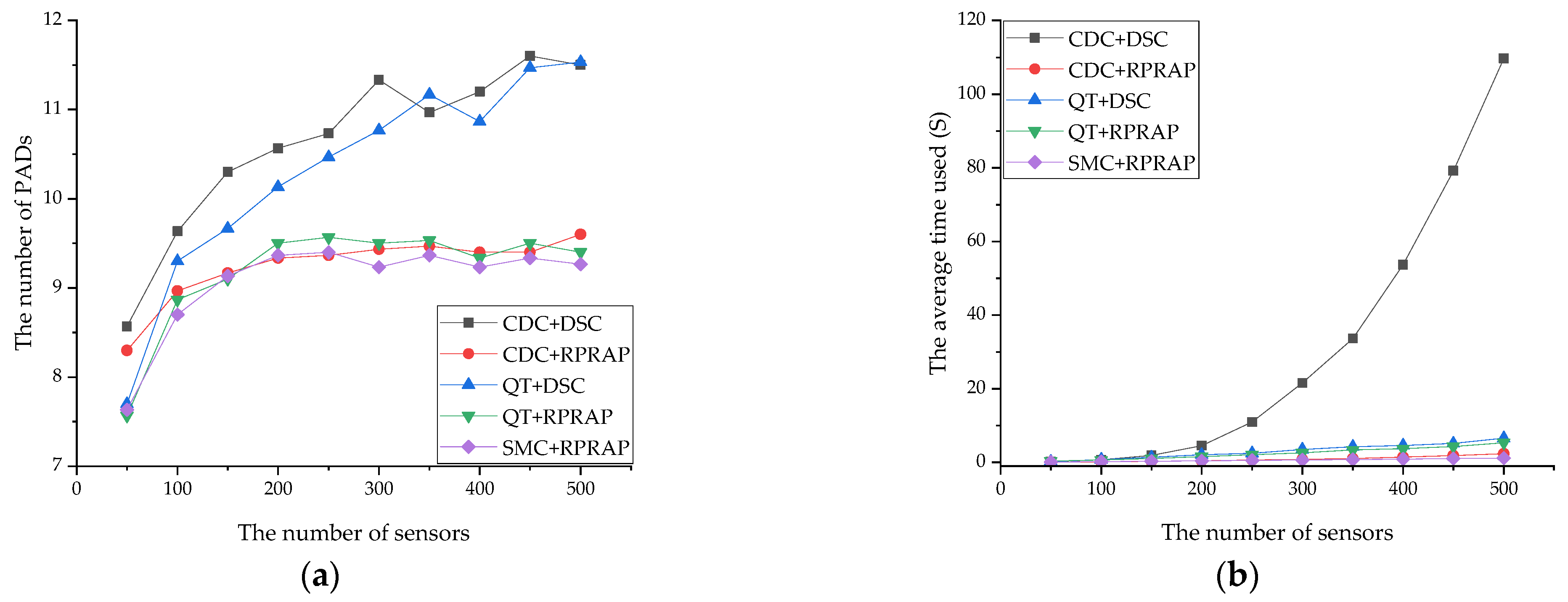
4.1. Performance Impact of Main Components of the Proposed Strategy

This work proposes several key mechanisms: the sink-outward allocation strategy, dynamic regional optimal search, and a redundant pad removal strategy called RPRAP. In studies by Chen et al. [5] and Cheng et al. [7], charging board deployment needed to consider the connectivity between new and existing ones. However, this work suggests ignoring connectivity during configuration and compares this approach with connectivity-considering ones.

In this section’s simulations, SMC+RPRAP represents our proposed method with all mechanisms. MC, SMC-O, SMC-C, and SMC-N respectively denote the versions after removing the sink-outward allocation strategy, RPRAP, ignoring connectivity during pad allocation, and dynamic regional optimal search mechanisms. Note that, apart from SMC-O, all other versions incorporate the RPRAP component. The omission of the RPRAP designation in their names is solely for the sake of simplicity. By comparing with SMC+RPRAP, the impact of each mechanism on performance is observed.

From Figure 3, Figure 4, Figure 5 and Figure 6, under four map sizes, SMC-N requires the most pads and the least execution time. Compared to SMC+RPRAP, it increases pad numbers by up to 55.00%, 98.20%, 80.90%, and 93.61% under the four maps, while reducing execution time by up to 92.79%, 97.23%, 96.58%, and 95.67%. This shows that although dynamic regional optimal search spends time finding optimal pad positions around target sensors, it effectively reduces pad numbers.

The second most pad-affecting mechanism is the redundant pad removal mechanism. Under the four map sizes, SMC-O increases pad numbers by up to 28.75%, 40.36%, 16.24%, and 5.01% compared to SMC+RPRAP while reducing execution time by up to 46.52%, 51.27%, 48.76%, and 57.91%.

The third is the inside-out configuration mechanism. Under the four map sizes, MC increases pad numbers by up to 12.20%, 24.46%, 13.01%, and 9.30% compared to SMC+RPRAP and reduces execution time by up to 39.83%, 44.22%, 33.75%, and 15.59%. The pad number gap tends to widen as sensor numbers increase.

Finally, under the four map sizes, compared to SMC+RPRAP, the pad number difference of SMC-C is nearly negligible in the 4096 × 4096 map, and execution time differences are mostly small. In the other three maps, SMC-C increases pad numbers by up to 7.58%, 8.12%, and 5.16%. In terms of time performance, among 30 environments, SMC-C only used less time in 7 cases, all with fewer sensors. Overall, SMC has a shorter execution time and fewer pads. Therefore, as expected, maintaining connectivity between newly added and configured charging boards during deployment is not necessary.

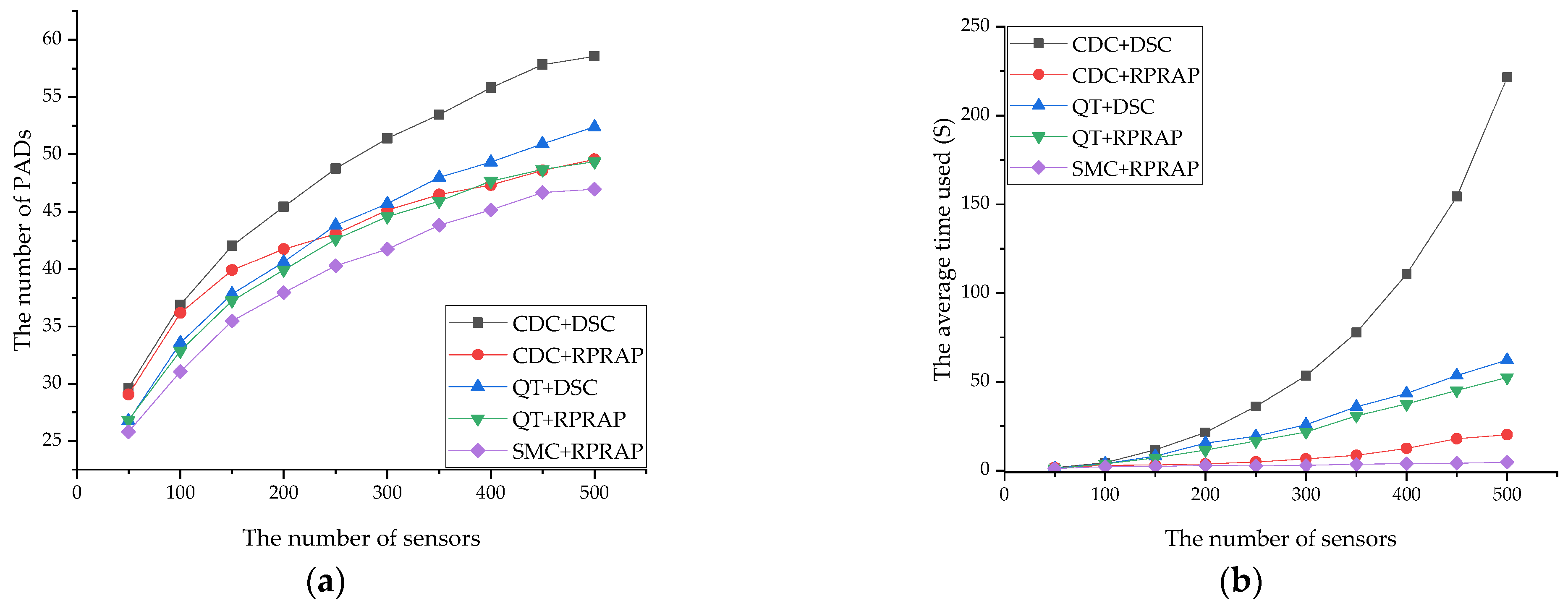
4.2. Performance Comparison

In the relevant literature, adding a redundant pad removal step can reduce the number of pads needed for configuration but will increase processing time. The QT method [7] uses the DSC algorithm [8] for removing redundant pads. Consequently, this section compares the proposed SMC+RPRAP method against CDC+DSC and QT+DSC. Algorithms such as MSC, TNC, and GNC, which were introduced in paper [5], have already been extensively compared with QT+DSC in paper [7] and are thus excluded from this analysis. As illustrated in Figure 7, Figure 8, Figure 9 and Figure 10, SMC+RPRAP demonstrates superior efficiency in pad utilization compared to both CDC+DSC and QT+DSC. Furthermore, the execution time of SMC+RPRAP is significantly reduced, being only a fraction of that of CDC+DSC and QT+DSC, which translates to a performance enhancement of several to tens of times faster.

As shown in Figure 7, Figure 8, Figure 9 and Figure 10, SMC+RPRAP reduces pad numbers by up to 10.61% (5.37 vs. 5.97), 19.54% (9.33 vs. 11.60), 17.27% (14.37 vs. 17.37), and 19.81% (58.57 vs. 46.97) compared to CDC+DSC. In terms of time efficiency, CDC+DSC shows increases of 6967.17% (33.27 vs. 0.48), 9873.93% (109.74 vs. 1.11), 8332.51% (129.70 vs. 1.56), and 5555.40% (221.48 vs. 3.99) over SMC+RPRAP. As discussed in [7], CDC generates numerous clusters, prolonging DSC processing time.

On the other hand, SMC+RPRAP outperforms QT+DSC in pad numbers by 11.11% (5.33 vs. 6.00), 19.65% (9.27 vs. 11.53), 10.64% (14.83 vs. 16.60), and 10.37% (46.97 vs. 52.40). QT+DSC has higher execution times than SMC+RPRAP by 488.63% (2.33 vs. 0.47), 593.49% (6.60 vs. 1.11), 772.95% (7.46 vs. 0.97), and 1561.28% (62.24 vs. 3.99). QT+DSC’s time consumption mainly comes from grid division and DSC-based redundant pad removal. With fewer generated pads, DSC takes less time than CDC+DSC. However, as the map size increases, QT requires more grid division time, widening the execution time gap with SMC+RPRAP.

As seen in the previous comparison, DSC took considerable time when handling numerous pads. What would the performance be if CDC and QT were paired with the RPRAP method proposed in this work for removing redundant pads? As shown in Figure 7, Figure 8, Figure 9 and Figure 10, CDC+RPRAP and QT+RPRAP represent the combination of CDC and QT with the proposed RPRAP method for removing redundant pads. As shown in Figure 7, Figure 8, Figure 9 and Figure 10, replacing DSC with RPRAP while using CDC reduces pad numbers and significantly cuts execution time. Except for the 4096 × 4096 map, where the maximum pad reduction was 9.94%, larger maps saw pad numbers drop by over 15% (18.97%, 15.38%, and 15.97%). Time reductions exceeded 90% in the best cases (97.23%, 97.85%, 96.68%, and 90.90%). Thus, RPRAP not only removes more redundant pads than DSC but also drastically reduces processing time when there are many deployed pads.

When QT is paired with RPRAP instead of DSC, in sparse scenarios (e.g., 150 sensors on a 4096 × 4096 map, 50 sensors on an 8192 × 8192 map, and 50 sensors on a 16384 × 16384 map), the average number of pads used slightly increased (by 0.61%, 1.83%, and 0.25%, respectively). However, in the majority of other cases, the usage of pads decreased. The maximum reductions reached 9.44%, 18.79%, 9.63%, and 5.79% across different maps. Execution times saw minimal increases in extremely sparse situations (e.g., 0.008196 s more for 50 sensors on a 4096 × 4096 map), while other cases showed reductions of up to 47.74%, 39.80%, 36.95%, and 25.66%. As map size grows, QT spends more time on grid division, so the time saved by using RPRAP decreases.

Notably, CDC+RPRAP and QT+RPRAP show varied pad number performance across maps, but the former has better execution times. Both CDC and QT combined with RPRAP, their performance approaches that of the proposed SMC+RPRAP. For CDC+RPRAP, in four of 40 test cases, it used fewer pads than SMC+RPRAP (by 2.38%, 0.58%, 0.36%, and 0.41%), though across the four maps, it used up to 3.66%, 8.73%, 13.55%, and 16.42% more pads. In terms of execution time, nine cases saw shorter times than SMC+RPRAP, with the extra time ranging from 0.96% to 26.24% in scenarios with fewer sensors. The maximum time increase over SMC+RPRAP was 93.16%, 99.02%, 159.71%, and 336.81% across the four maps.

For QT+RPRAP, three of the 40 test cases used fewer pads than SMC+RPRAP (by 0.36%, 0.81%, and 0.40%), but across the four maps, it used up to 6.49%, 3.45%, 7.42%, and 6.79% more. Execution time was lower than SMC+RPRAP only in the 16384 × 16384 map with 50 sensors (by 4.67%). Across the four maps, the maximum time increases over SMC+RPRAP were significant—191.72%, 272.86%, 463.79%, and 1034.08%.

In summary, SMC+RPRAP generally outperforms CDC+RPRAP and QT+RPRAP in pad configuration and execution time. However, it shows room for improvement in ensuring pad connectivity, especially in cases with fewer sensors where execution times were longer.

4.3. The Impact of Obstacle Areas

In some regions, the presence of terrain features or buildings may make it impossible to construct pads. To handle obstacle areas, this paper proposes a method that integrates critical checks into two key algorithms: AdjPadPos and ConnectPads. In AdjPadPos (Line 5, Algorithm 2), it strictly prohibits placing pads within obstacle regions. In ConnectPads, three crucial lines (Lines 9, 16, and 23 of Algorithm 3) enforce two rules: endpoint pads cannot be moved into obstacle areas, and no connection pads can be inserted there. These algorithmic checks effectively prevent any pad-related operations in obstacle areas, ensuring a more reliable design process. When the obstacle area is too large to be traversed by drones, the ConnectPad algorithm must consider how to bypass the obstacle area, and there may even be complex issues such as the inability to connect. These scenarios will be further explored in our future work.

Figure 11 shows the number of pads and execution time required by the SMC+RPRAP method when using four different map sizes with a randomly generated circular obstacle area of radius 1000 m and 50 to 500 sensors uniformly and randomly distributed in the non-obstacle areas of the maps. The legend naming convention is map size–obstacle area count; for example, 4906-0 indicates a 4096 × 4096 map with no obstacle areas. Figure 11a shows that because there are no sensors in the obstacle area, the area available for sensor distribution is reduced, making the sensors relatively denser and thus requiring fewer pads. However, as previously mentioned, an increase in the number and size of obstacle areas may lead to pad connectivity issues. On the other hand, although AdjPadPos and ConnectPads need to avoid placing pads in obstacle locations, the obstacle areas also reduce the area available for sensor distribution (as seen in the experiments in Section 4.2, smaller maps require less time), so Figure 11b shows that adding an obstacle area does not necessarily increase the execution time.

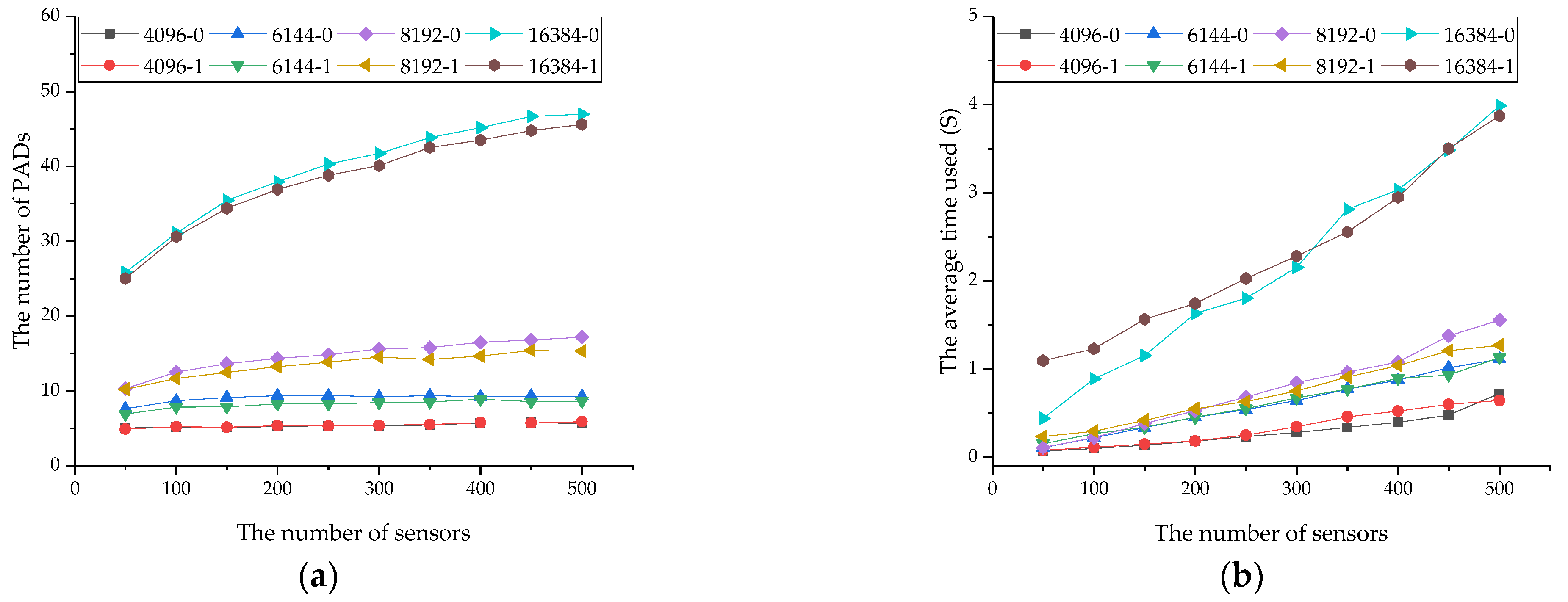
4.4. The Impact of Grid Granularity Setting on Performance

In the algorithm AdjPadPos, we search for the optimal placement locations near the target sensors. The granularity of the search affects both the quality of the found locations and the execution time. In this section, we set the search interval to 25, 50, 100, 150, and 200, respectively, and tested on a 16,384 × 16,384 map using SMC+RPRAP.

Figure 12 shows that as the grid interval increases, the number of pads in the final configuration tends to increase, while the execution time, as expected, decreases. An interval of 100 is a compromise between the execution time and the number of pads. Therefore, in the experiments of this paper, the grid interval is set to 100.

5. Conclusions

In this work, we proposed a novel sink-outward strategy for efficient charging pad deployment in large-scale wireless rechargeable sensor networks (WRSNs). Our approach, termed sink-outward max covering (SMC), along with the optimization step—reducing pads by reallocating pads partially (RPRAP)—demonstrated significant advantages in minimizing the number of deployed charging pads while ensuring network connectivity and coverage. Overall, the proposed strategy offers a more effective and efficient solution for charging pad deployment in large-scale WRSNs. Future work could explore further optimization of pad connectivity and the application of this strategy in more complex network scenarios.

Deploying advanced wireless charging pads in the future represents a substantial challenge. For example, the wireless charging pad is equipped with multiple docking stations so that multiple wireless charging drones can land and be charged simultaneously on the same pad. Moreover, deploying high-power and high-cost wireless charging pads also makes the optimization problem more complicated. In this work, the wireless charging vehicles were applied to charge some mobile sensors that were far away from a wireless charging pad. In the future, we may consider deploying vehicles (cars) mounted with a wireless charging pad in a large-scale WRSN to support real-time wireless charging services for wireless charging drones.

References

1. Akyildiz, I.F.; Su, W.; Sankarasubramaniam, Y.; Cayirci, E. A Survey on Sensor Networks. IEEE Commun. Mag. 2002, 40, 102–114. [Google Scholar] [CrossRef]
2. Zhao, M.; Li, J.; Yang, Y. A framework of joint mobile energy replenishment and data gathering in wireless rechargeable sensor networks. IEEE Trans. Mob. Comput. 2014, 13, 2689–2705. [Google Scholar] [CrossRef]
3. Lin, C.; Zhou, J.; Guo, C.; Song, H.; Wu, G.; Obaidat, M.S. TSCA: A Temporal-Spatial Real-Time Charging Scheduling Algorithm for On-Demand Architecture in Wireless Rechargeable Sensor Networks. IEEE Trans. Mob. Comput. 2017, 17, 211–224. [Google Scholar] [CrossRef]
4. Rong, C.; Duan, X.; Chen, M.; Wang, Q.; Yan, L.; Wang, H.; Xia, C.; He, X.; Zeng, Y.; Liao, Z. Critical Review of Recent Development of Wireless Power Transfer Technology for Unmanned Aerial Vehicles. IEEE Access 2023, 11, 132982–133003. [Google Scholar] [CrossRef]
5. Chen, J.; Yu, C.W.; Ouyang, W. Efficient Wireless Charging Pad Deployment in Wireless Rechargeable Sensor Networks. IEEE Access 2020, 8, 39056–39077. [Google Scholar] [CrossRef]
6. Baek, J.; Han, S.I.; Han, Y. Optimal UAV Route in Wireless Charging Sensor Networks. IEEE Internet Things J. 2020, 7, 1327–1335. [Google Scholar] [CrossRef]
7. Cheng, R.-H.; Yu, C.W.; Zhang, Z.-L. Optimizing Charging Pad Deployment by Applying a Quad-Tree Scheme. Algorithms 2024, 17, 264. [Google Scholar] [CrossRef]
8. Chen, Y.; Gu, Y.; Li, P.; Lin, F. Minimizing the Number of Wireless Charging PAD for UAV-Based Wireless Rechargeable Sensor Networks. Int. J. Distrib. Sens. Netw. 2021, 17, 15501477211055958. [Google Scholar] [CrossRef]
9. Slhu, Y.; Yousefi, H.; Cheng, P.; Chen, J.; Gu, Y.; He, T.; Shin, K.G. Near-optimal velocity control for mobile charging in wireless rechargeable sensor networks. IEEE Trans. Mob. Comput. 2015, 15, 1699–1713. [Google Scholar]
10. Fu, L.; He, L.; Cheng, P.; Gu, Y.; Pan, J.; Chen, J. ESync: Energy Synchronized Mobile Charging in Rechargeable Wireless Sensor Networks. IEEE Trans. Veh. Technol. 2015, 65, 7415–7431. [Google Scholar] [CrossRef]
11. Cheng, R.-H.; Yu, C.W.; Xu, C.J.; Wu, T.-K. A Distance-Based Scheduling Algorithm with a Proactive Bottleneck Removal Mechanism for Wireless Rechargeable Sensor Networks. IEEE Access 2020, 8, 148906–148925. [Google Scholar] [CrossRef]
12. Wang, C.; Li, J.; Yang, Y. Low-latency mobile data collection for wireless rechargeable sensor networks. In Proceedings of the IEEE International Conference on Communications (IEEE ICC), London, UK, 8–12 June 2015; pp. 6524–6529. [Google Scholar]
13. Xie, L.; Shi, Y.; Hou, Y.T.; Lou, A. Wireless poser transfer and applications to sensor networks. IEEE Wirel. Commun. 2013, 20, 140–145. [Google Scholar]
14. Xie, L.; Shi, Y.; Hou, Y.T.; Lou, W.; Sherali, H.D. On traveling path and related problems for a mobile station in a rechargeable sensor network. In Proceedings of the 14th ACM International Symposium on Mobile Ad Hoc Networking and Computing (Mobihoc), Bangalore, India, 29 July–1 August 2013; pp. 109–118. [Google Scholar]
15. Guo, P.; Liu, X.; Tang, S.; Cao, J. Concurrently wireless charging sensor networks with efficient scheduling. IEEE Trans. Mob. Comput. 2017, 16, 2450–2463. [Google Scholar] [CrossRef]
16. Zorbas, D.; Douligeris, C. Computing drone positions to wirelessly recharge IoT devices. In Proceedings of the IEEE INFOCOM 2018—IEEE Conference on Computer Communications Workshops (INFOCOM WKSHPS), Honolulu, HI, USA, 15–19 April 2018; pp. 628–633. [Google Scholar]
17. Lin, T.-L.; Chang, H.-Y.; Wang, Y.-H. A Novel Unmanned Aerial Vehicle Charging Scheme for Wireless Rechargeable Sensor Networks in an Urban Bus System. Electronics 2022, 11, 1464. [Google Scholar] [CrossRef]
18. Chen, J.; Yu, C.W.; Cheng, R.-H. Collaborative Hybrid Charging Scheduling in Wireless Rechargeable Sensor Networks. IEEE Trans. Veh. Technol. 2022, 71, 8994–9010. [Google Scholar] [CrossRef]
19. Wibotic. PowerPad. Available online: https://www.wibotic.com/products/powerpad/ (accessed on 1 March 2025).
20. Skysense. Charging Pad Outdoor Specs. Available online: https://www.skysense.co/charging-pad-outdoor/specs (accessed on 1 March 2025).
21. Getcorp. In-Flight Wireless Charging Outdoor Demonstration. Available online: http://getcorp.com/in-flight-wireless-charging-outdoor-demonstration/ (accessed on 1 March 2025).
22. Long, T.; Ozger, M.; Cetinkaya, O.; Akan, O.B. Energy Neutral Internet of Drones. IEEE Commun. Mag. 2018, 56, 22–28. [Google Scholar] [CrossRef]
23. Xing, Y.; Young, R.; Nguyen, G.; Lefebvre, M.; Zhao, T.; Pan, H.; Dong, L. Optimal Path Planning for Wireless Power Transfer Robot Using Area Division Deep Reinforcement Learning. Wirel. Power Transf. 2022, 9, 21885. [Google Scholar] [CrossRef]
24. Bui, N.; Le Nguyen, P.; Nguyen, V.A.; Do, P.T. A Deep Reinforcement Learning-based Adaptive Charging Policy for WRSNs. arXiv 2022, arXiv:2208.07824. [Google Scholar]
25. Nowrozian, N.; Tashtarian, F.; Forghani, Y. On Optimizing the Charging Trajectory of Mobile Chargers in Wireless Sensor Networks: A Deep Reinforcement Learning Approach. Wirel. Netw. 2023, 30, 421–436. [Google Scholar] [CrossRef]
26. Lee, H.; Ji, D.; Cho, D.-H. Optimal Design of Wireless Charging Electric Bus System Based on Reinforcement Learning. Energies 2019, 12, 1229. [Google Scholar] [CrossRef]
27. Suman, S.; Kumar, S.; De, S. Path Loss Model for UAV-Assisted RFET. IEEE Commun. Lett. 2018, 22, 2048–2051. [Google Scholar] [CrossRef]
28. Dijkstra, E.W. A note on two problems in connexion with graphs. Numer. Math. 1959, 1, 269–271. [Google Scholar] [CrossRef]
Figure 1. Workflow diagram of sink-outward charging pad deployment.
Electronics 14 02159 g001
Figure 2. Illustration of the grid area for optimal pad placement around the target sensor.
Electronics 14 02159 g002
Figure 3. Impact of the proposed strategy’s components on (a) the number of pads and (b) average execution time on small-scale maps.
Electronics 14 02159 g003
Figure 4. Impact of the proposed strategy’s components on (a) the number of pads and (b) average execution time on medium-scale maps.
Electronics 14 02159 g004
Figure 5. Impact of the proposed strategy’s components on (a) the number of pads and (b) average execution time on large-scale maps.
Electronics 14 02159 g005
Figure 6. Impact of the proposed strategy’s components on (a) the number of pads and (b) average execution time on extremely large-scale maps.
Electronics 14 02159 g006
Figure 7. Comparison of different algorithms in terms of (a) the number of pads and (b) average execution time on small-scale maps.
Electronics 14 02159 g007
Figure 8. Comparison of different algorithms in terms of (a) the number of pads and (b) average execution time on medium-scale maps.
Electronics 14 02159 g008
Figure 9. Comparison of different algorithms in terms of (a) the number of pads and (b) average execution time on large-scale maps.
Electronics 14 02159 g009
Figure 10. Comparison of different algorithms in terms of (a) the number of pads and (b) average execution time on extremely large-scale maps.
Electronics 14 02159 g010
Figure 11. Comparison of the performance of SMC+RPRAP in terms of (a) the number of pads and (b) average execution time in maps of different sizes with 0 to 1 circular obstacle areas of radius 1000 m.
Electronics 14 02159 g011
Figure 12. Comparison of the performance impact on (a) the number of pads and (b) average execution time when using different grid search intervals in the algorithm AdjPadPos for extremely large-scale maps.
Electronics 14 02159 g012