A Hybrid TDOA and AOA Visible Light Indoor Localization Method Using IRS

Abstract

Traditional wireless positioning techniques often suffer from accuracy degradation in indoor environments due to multipath effects and occlusion. To address this issue, this paper proposes an indoor positioning method for visible light communication (VLC) combined with intelligent reflective surface (IRS) assistance to improve the positioning accuracy and stability in complex environments. This work proposes the concepts of a virtual source and virtual receiver based on IRS and conducts positioning optimization by combining the measurements of the time difference of arrival (TDOA) and angle of arrival (AOA). The research adopts a semi-positive definite relaxation (SDR) optimization method to efficiently solve the nonlinear optimization problem, ensuring the global convergence and accuracy of the algorithm. Meanwhile, the weights of the positioning results of the virtual light source and the real light source are dynamically adjusted by using the distance residual, thereby reducing the influence of measurement noise. Monte Carlo simulation experiments demonstrate the advantages of the proposed method in terms of the positioning error and robustness compared with traditional positioning algorithms in the environment of large noise interference. The experimental results demonstrate the efficacy of the method in addressing multipath and occlusion issues, while also exhibiting notable adaptability and stability across diverse hardware configurations.

1. Introduction

Recently, with the rapid development of the Internet of Things and industrial technology, high-precision indoor positioning technology has become increasingly important in fields such as smart home, industrial automation, intelligent storage, and indoor navigation [1,2,3]. However, traditional wireless positioning technologies, such as Wi-Fi, Bluetooth, and ultra-wideband (UWB), are vulnerable to electromagnetic signal interference generated by other radio frequency wireless devices and also require additional infrastructure [1,4]. In contrast, visible light communication (VLC) technology has become a research hotspot that attracts much attention in the field of indoor positioning in recent years due to its advantages such as wide bandwidth, strong anti-interference ability, low cost, and high security [5,6,7]. However, to achieve high precision visible light positioning, the system must obtain accurate information about light-emitting diodes’ (LEDs) deployment in advance [8]. At present, such information usually relies on architectural drawings or manual measurements, but the former is often inaccurate and lacks electronic identifiers, and the latter faces problems such as a high labor cost and low efficiency and can be error-prone in large-scale deployment, which seriously restricts the practical application of visible light positioning (VLP) systems [9].

The localization of LEDs is essentially a passive localization problem, and the localization process is performed by taking different types of measurements of the signal sources from stations with known locations and then solving the source locations using localization algorithms [5]. The measurement information includes the received signal strength (RSS), time of arrival (TOA), time difference of arrival (TDOA), and angle of arrival (AOA) [10,11,12,13]. However, the positioning accuracy of a single measurement method is limited, so the hybrid TDOA-AOA positioning method has been widely researched in recent years [14,15,16,17,18]. Reference [14] proposed a hybrid TDOA-AOA source localization approach that achieves higher accuracy than using either TDOA or AOA alone. In ref. [15], a constrained optimization method with geometric constraints was applied to the hybrid model, offering better robustness than traditional linear least squares. Reference [16] presented a closed-form localization solution combining TDOA and AOA measurements, particularly effective in low-probability-of-intercept environments. Reference [17] introduced a structured total least squares method to reduce the estimation bias in hybrid localization problems. Reference [18] proposed a hybrid positioning method based on multi-station TDOA and single-station AOA. This approach enhanced the positioning accuracy by incorporating AOA measurement information into TDOA equations and utilizing the weighted least square method to solve for the closed solution. Consequently, enhanced stability and accuracy can be achieved, surpassing the capabilities of single-station AOA. Nevertheless, this method may not achieve optimal results in environments characterized by significant multipath and occlusion effects.

Furthermore, whether it is TDOA or AOA, the direct relationship between the measured value and the source position is nonlinear and non-convex [19,20]. Directly solving it using nonlinear methods will lead to an increase in computational complexity. Among the existing methods, the most classic algorithms are solved through some non-iterative techniques [21,22]. For example, the two-stage weighted least squares (TWLS) method [21] estimates the target position and auxiliary variables by rearranging the nonlinear TDOA equations into a set of linear equations while ignoring the relationship between the target position and the auxiliary variables and then refines the estimates. Although non-iterative methods have high computational efficiency, they are sensitive to measurement noise. Although the iterative optimization method can improve the accuracy, there exists the problem of convergence [18,23]. For example, the iterative constrained weighted least squares (lCWLS) method [23] takes the relationship between the target position and the auxiliary variables as the constraint and iteratively updates the weight matrix. However, this method faces the divergence problem.

More critically, most of the existing algorithms are based on the hypothesis of line-of-sight (LOS) propagation, but in the actual indoor environment, the signal is often reflected and refracted by obstacles to form non-line-of-sight (NLOS) propagation, resulting in increased measurement errors and seriously affecting the positioning performance.

In recent years, the rise of intelligent reflective surface (IRS) technology has provided a new way to solve the signal enhancement problem in an NLOS environment [24,25]. An IRS can actively regulate the electromagnetic wave propagation environment and optimize the signal quality of the reflection path [26]. Several studies have demonstrated the potential of an IRS in enhancing the VLP accuracy and reliability. Reference [27] analyzed the impact of meta surfaces and mirror arrays in IRS-assisted VLC and showed a significant improvement in signal coverage. Reference [28] proposed a passive indoor localization system using an IRS and verified its effectiveness in practical environments. Reference [29] proposed an RSS-based n-step method for VLP in combination with an IRS, according to high localization accuracy in the NLOS case. Previous studies have demonstrated the effectiveness of an IRS in enhancing VLP systems, achieving improved accuracy and robustness. However, most of these studies are based on RSS algorithms, and there are fewer studies on TDOA and AOA algorithms.

While RSS-based positioning methods are indeed simpler to implement, they typically suffer from lower accuracy and higher susceptibility to multipath fading and noise, particularly in complex indoor environments. In contrast, TDOA provides geometric information that is less sensitive to power fluctuations, and AOA offers direct directional cues. By combining TDOA and AOA, the proposed method harnesses both range-difference and angular diversity, which significantly enhances the positioning robustness and precision. Despite its potential, the existing research has yet to fully explore how an IRS can be systematically integrated into a hybrid TDOA-AOA VLC localization framework.

In summary, the problem of low-cost and high-precision source localization in complex indoor scenarios remains a difficult issue that needs to be studied and implemented. Based on the above situation, this paper studies the feasibility of deploying an IRS in the indoor VLP system and proposes a high-precision indoor positioning method based on TDOA and AOA suitable for this scenario. The proposed system integrates TDOA and AOA measurements using a PD-based receiver array. The IRS module adopts a passive specular reflection design. Compared to UWB systems, our solution offers a lower deployment cost, and compared to RSS-based VLC approaches, it achieves significantly higher accuracy and robustness. This cost–performance balance makes it well-suited for industrial automation, smart lighting, and medical navigation applications that require sub-meter indoor localization. Specifically, the contributions of the paper are summarized as follows:

• A virtual path modeling method based on an IRS was proposed. By establishing virtual light source and virtual receiver models, the NLOS path was transformed into a virtual LOS path. Combined with the measurement information of TDOA and AOA, the geometric symmetry of the IRS was utilized to improve the solution ability of the positioning equation.
• We designed an optimization algorithm based on semi-positive definite relaxation (SDR), which transforms the non-convex positioning problem into a semi-definite programming (SDP) problem. By introducing the initial weighted least squares (WLS) estimation and the IRS reflection path length constraint, as well as relaxing the rank constraint, the convexity and global convergence of the optimization problem are guaranteed.
• A dynamic weighted fusion strategy was proposed, which utilizes the distance residual to dynamically adjust the weights of the positioning results of the virtual light source and the real light source, in order to effectively suppress the influence of measurement noise.

The remainder of this paper is organized as follows. Section 2 presents the system model, including the channel gain and the localization scenario. Section 3 details the proposed hybrid TDOA-AOA localization method, including the mathematical formulation, optimization algorithm, and implementation strategy. Section 4 provides the simulation results and performance evaluations under various conditions. Finally, Section 5 concludes the paper and discusses future work.

In this paper, bold uppercase and lowercase letters are used to denote the matrix and column, respectively. The term ${\mathbf{A}}_{i,j}$ denotes the i-th row and j-th column element of the matrix $\mathbf{A}$. The term ${\left|\right|\mathbf{a}\left|\right|}_2$ is the Euclidean norm, $diag\left(\mathbf{a}\right)$ is the diagonal matrix of the elements of $\mathbf{a}$, and $blkdiag\left(\mathbf{A}\dots \mathbf{B}\right)$ is written as $\mathbf{A}\dots \mathbf{B}$. $blkdiag\left(\mathbf{A},\dots ,\mathbf{B}\right)$ is a diagonal matrix consisting of $\mathbf{A},\dots ,\mathbf{B}$. $tr\left(\mathbf{A}\right)$ represents the determinant and trace of $\mathbf{A}$, respectively. $\mathbf{I}$ and $\mathbf{O}$ represent identity and zero matrices, respectively, and their subscripts denote the matrix size. Vectors ${\mathbf{1}}_N$ and ${\mathbf{0}}_N$ are defined as having a length of N and are expressed in unity and zero, respectively.

2. System Model

2.1. Channel Gain

First, we characterized the indoor model with an LED fixed to the ceiling, as this layout is commonly adopted in VLC systems. Figure 1 shows the proposed indoor positioning model. The IRS is mounted on one side of the wall. The channel of this model consists of LOS and NLOS paths. The LOS channel direct gain in a VLC usually follows the Lambertian model [27,29], which is widely used in VLC and indoor localization to describe the directional radiation pattern of an LED. It assumes that the emitted optical power varies with the cosine of the angle between the light direction and the surface normal, which is mathematically given by

$$h_{LOS}={\displaystyle \frac{(m+1)A}{2\pi d_{l,p}^2}}{cos}^m\left({\theta }_1\right)g_{of}cos\left({\varphi }_1\right)f_{oc},$$

(1)

where $m=-1/lo{g}_2(cos\left({\Theta }_{1/2}\right))$ is the Lambertian index, with ${\Theta }_{1/2}$ as the semi-angle at half illuminance of the LED, A is the receiving area of the photodetector (PD), $d_{l,p}$ is the distance between the transceivers, and ${\theta }_1$ and ${\varphi }_1$ are the angles of irradiance and incidence of the LED to PD, respectively. $g_{of}$ is the optical filter gain, and $f_{oc}$ is the optical concentration gain.

Generally, NLOS paths in wireless communication include the reflection path, diffraction path, and penetration path. Given the extremely high permeability loss and nanometer wavelength of visible light, the penetration path and diffraction path are usually ignored in a VLC. According to the surface characteristics of the reflector, the light reflection can be divided into two types: diffuse reflection and specular reflection. However, it turns out that the path loss of the secondary diffused reflection is 25 dB larger than that of the LOS path, and even the gain of the single-hop diffused reflection path is 15 dB lower than that of the LOS path. As a result, specular reflection is often considered an important NLOS component in IRS-assisted VLC, while diffuse reflection is ignored.

In specular reflection, the irradiation angle is equal to the incident angle, which is also called Snell’s reflection law. The upper bound of irradiance obtained under the point source condition is [27]

$$E={\displaystyle \frac{\mathit{\delta }(m+1)p{cos}^m\left(\theta \right)}{2\pi {(d_{l,i}+d_{i,p})}^2}}cos\left(\varphi \right),$$

(2)

where $\mathit{\delta }$ and p are the reflection factor and the emission power, $d_{l,i}$ is the distance between the LED and the IRS, and $d_{i,p}$ is the distance between the IRS and the PD.

Considering the nanoscale wavelength in VLC, the signal propagation distance in an indoor environment is less than the threshold $L_0$ of the near and far fields as shown in the following formula [30]:

$$L_0={\displaystyle \frac{2D^2}{\lambda }},$$

(3)

where D and $\lambda$ represent the maximum size of the IRS and the wavelength of the signal, respectively. Then, the near field assumption is ensured in IRS-aided VLC.

Based on Equations (2) and (3), the NLOS channel gain can be written as

$$h_{NLOS}=\mathit{\delta }{\displaystyle \frac{(m+1)A}{2\pi {(d_{l,i}+d_{i,p})}^2}}{cos}^m\left({\theta }_2\right)g_{of}cos\left({\varphi }_2\right)f_{oc}.$$

(4)

2.2. Localization Scenario

In the system, first, we assume that the receiver array receives only LOS signals, and then we use the rotation of the IRS to make it receive NLOS path signals. Since the two paths have different propagation delay characteristics, the system can indirectly extract the arrival time difference of the reflected path through the TDOA change measured by the receiver before and after receiving the signal from the NLOS path. Combining the geometrical position and control angle of the IRS, we can establish an equivalent model of IRS paths. Equation (4) demonstrates that the specular reflection path can be equivalent to an extended path consisting of a mirrored LED to PD link. As shown in Figure 2, $s_2$ and $P^{\prime }$ are the virtual mirror source and virtual station of source $s_1$ and the real PD, respectively. The reflection path $d_2+d_3$ is equivalent to the direct path $d_4+d_3$ from $s_2$ to P, as well as the direct path $d_2+d_5$ from $s_1$ to $P^{\prime }$. $d_6$ is the virtual LOS path.

The establishment of a virtual source and virtual PD needs to be based on the location of the IRS in space and also depends on the IRS geometry and rotation angle. As demonstrated in Figure 3, the IRS employs a compact folded actuator design to adjust its rotation angle by electrostatic actuation, thereby enabling a wide range of operations, including wavefront shaping and beam steering. Figure 3 shows the rotation of the IRS around an axis parallel to the x and z axes at its center point, respectively. To ensure the validity of the specular reflection assumption, the IRS rotation angles $\theta \in ({\theta }_{min},{\theta }_{max})$ and $\phi \in ({\phi }_{min},{\phi }_{max})$ are constrained within a pre-defined range. These bounds are selected based on the receiver and spatial geometry to ensure that the reflected beams remain physically receivable by the PD array.

Consider the IRS shown in Figure 2; with its normal vector ${\mathbf{n}}_{\mathbf{y}}={(0,1,0)}^T$, all possible directions towards the interior of the room can be obtained when it is rotated about the x and z axes. The new direction can be obtained by

$${\mathbf{n}}_{\mathbf{y}}^{\ast }={\mathbf{R}}_{\mathbf{x}}{\mathbf{R}}_{\mathbf{z}}{\mathbf{n}}_{\mathbf{y}},$$

(5)

where

$${\mathbf{R}}_{\mathbf{x}}=\left[\begin{array}{ccc}1& 0& 0\\ 0& cos\left(\theta \right)& -sin\left(\theta \right)\\ 0& sin\left(\theta \right)& cos\left(\theta \right)\end{array}\right],{\mathbf{R}}_{\mathbf{z}}=\left[\begin{array}{ccc}cos\left(\phi \right)& -sin\left(\phi \right)& 0\\ sin\left(\phi \right)& cos\left(\phi \right)& 0\\ 0& 0& 1\end{array}\right].$$

(6)

Assume that the IRS center point is $\mathbf{C}$ and the point with known coordinates outside the IRS plane is $\mathbf{P}$. The coordinate ${\mathbf{P}}^{\prime }$ of $\mathbf{P}$ with respect to the rotated IRS symmetry can be obtained by

$${\mathbf{P}}^{\prime }=\mathbf{P}-2·{\displaystyle \frac{{\mathbf{n}}_{\mathbf{y}}^{\ast }·\left(\mathbf{P}-\mathbf{C}\right)}{\parallel {\mathbf{n}}_{\mathbf{y}}^{\ast }{\parallel }^2}}·{\mathbf{n}}_{\mathbf{y}}^{\ast }.$$

(7)

Considering the complexity of the indoor environment, decentralized deployment of PDs is not conducive to localization. Moreover, the range of IRS reflection signals that can be received at a fixed time is limited, and the distributed PD may not be able to simultaneously receive reflection signals at the same time. The rotatable sensor array shown in Figure 4 is used for source localization [13].

The receiver deploys five PDs and one AOA sensor, the PDs are located in the center of the top surface and the four sides, and the AOA sensor is arranged on the top surface, sharing coordinates with the PD1. The receiver array can be rotated around the y and x axes, similar to the IRS rotation, and the coordinates after rotation can be obtained using the rotation matrix of Equation (6). $\alpha$ represents the base angle of the longitudinal cross section of the receiver, and the relationship between the field of view (FOV) satisfies Equation (8) to maximize the reception of incident light from the target.

$$\alpha +FOV={\displaystyle \frac{\pi }{2}}$$

(8)

3. Localization Method

3.1. The Closed-Form Solution for Source Localization

The position coordinates of the $i_{th}$ PD in a three-dimensional space are represented by the vector ${\mathbf{p}}_{\mathbf{i}}={[x_i,y_i,z_i]}^T,i=1,2,\dots ,N$. The coordinates of the signal source ${\mathbf{s}}_{\mathbf{1}}$ and the virtual signal source ${\mathbf{s}}_{\mathbf{2}}$ obtained by IRS reflection are represented by the vector ${\mathbf{s}}_{\mathbf{k}}={[x_{x,k},y_{y,k},z_{z,k}]}^T,k=1,2$. The distance from source $s_k$ to receiving station $p_i$ is given by the following equation:

$$d_{i,k}={\left|\right|{\mathbf{p}}_{\mathbf{i}}-{\mathbf{s}}_{\mathbf{k}}\left|\right|}_2.$$

(9)

Without loss of generality, taking the first PD as the reference station, the difference in distance from the signal source to the $i_{th}$ PD and the reference PD is given by

$$d_{i1,k}=d_{i,k}-d_{1,k},i=2,\dots ,N.$$

(10)

The TDOA localization method is the primary subject of study. By shifting the variable $d_{1,k}$ from the right-hand side of Equation (10) to the left-hand side and subsequently squaring both sides, the operation can be obtained as follows:

$${({\mathbf{p}}_{\mathbf{i}}-{\mathbf{p}}_{\mathbf{1}})}^T({\mathbf{s}}_{\mathbf{k}}-{\mathbf{p}}_{\mathbf{1}})+d_{i1,k}{d}_{1,k}=0.5[{({\mathbf{p}}_{\mathbf{i}}-{\mathbf{p}}_{\mathbf{1}})}^T({\mathbf{p}}_{\mathbf{i}}-{\mathbf{p}}_{\mathbf{1}})-d_{i1,k}^2].$$

(11)

For the sake of expediency, the auxiliary vector $\mathbf{u}={[{({\mathbf{s}}_{\mathbf{1}}-{\mathbf{p}}_{\mathbf{1}})}^T,{({\mathbf{s}}_{\mathbf{2}}-{\mathbf{p}}_{\mathbf{1}})}^T,d_{1,1},d_{1,2}]}^T$ is first defined, after which Equation (11) can be written in matrix form.

$${\mathbf{h}}_{\mathbf{t}}={\mathbf{G}}_{\mathbf{t}}\mathbf{u}$$

(12)

$${\mathbf{G}}_{\mathbf{t}}=\left[\begin{array}{cccc}\mathbf{R}& {\mathbf{O}}_{(\mathbf{N}-\mathbf{1})\times \mathbf{3}}& {\mathbf{d}}_{\mathbf{1}}& {\mathbf{0}}_{\mathbf{N}-\mathbf{1}}\\ {\mathbf{O}}_{(\mathbf{N}-\mathbf{1})\times \mathbf{3}}& \mathbf{R}& {\mathbf{0}}_{\mathbf{N}-\mathbf{1}}& {\mathbf{d}}_{\mathbf{2}}\end{array}\right],$$

(13)

$${\mathbf{h}}_{\mathbf{t}}=\left[\begin{array}{c}{\mathbf{h}}_{\mathbf{1}}\\ {\mathbf{h}}_{\mathbf{2}}\end{array}\right]$$

(14)

where $\mathbf{R}={[{\mathbf{p}}_{\mathbf{2}}-{\mathbf{p}}_{\mathbf{1}},...,{\mathbf{p}}_{\mathbf{N}}-{\mathbf{p}}_{\mathbf{1}}]}^T$, ${\mathbf{d}}_{\mathbf{k}}={[d_{21,k},\dots ,d_{N1,k}]}^T$, and ${\mathbf{h}}_{\mathbf{k}}={\displaystyle \frac{1}{2}}[{({\mathbf{p}}_{\mathbf{2}}-{\mathbf{p}}_{\mathbf{1}})}^T({\mathbf{p}}_{\mathbf{2}}-{\mathbf{p}}_{\mathbf{1}})$ $-d_{21,k}^2,\dots ,{({\mathbf{p}}_{\mathbf{N}}-{\mathbf{p}}_{\mathbf{1}})}^T({\mathbf{p}}_{\mathbf{N}}-{\mathbf{p}}_{\mathbf{1}})-d_{N1,k}^2{]}^T,k=1,2$.

Equation (12) is established without noise. However, in practical engineering applications and scientific research, measurements are often inevitably disturbed by noise. ${\tilde{\mathbf{h}}}_{\mathbf{t}}$ and ${\tilde{\mathbf{G}}}_{\mathbf{t}}$, respectively, represent measurements affected by noise. With the first-order Taylor expansion of the formula, we can obtain a pseudo-linear equation.

$${\tilde{\mathbf{G}}}_{\mathbf{t}}\mathbf{u}-{\tilde{\mathbf{h}}}_{\mathbf{t}}\approx \eta$$

(15)

$$\eta =\left[\begin{array}{c}{\mathbf{B}}_1{\mathbf{n}}_1\\ {\mathbf{B}}_2{\mathbf{n}}_2\end{array}\right],$$

(16)

where $\eta =\mathbf{Bn}$ is the error term, $\mathbf{B}=blkdiag({\mathbf{B}}_{\mathbf{1}},{\mathbf{B}}_{\mathbf{2}})$, ${\mathbf{B}}_{\mathbf{k}}=diag\left[d_{2,k,}{d}_{3,k},d_{4,k},d_{5,k}\right]$, and $\mathbf{n}={\left[{\mathbf{n}}_{\mathbf{1}}^T,{\mathbf{n}}_{\mathbf{2}}^T\right]}^T$ represents the measurement error, which follows a Gaussian distribution with a mean of zero and a covariance matrix denoted as ${\mathbf{Q}}_t$, ${\mathbf{n}}_{\mathbf{k}}={\left[n_{21,k,}{n}_{31,k},n_{41,k},n_{51,k}\right]}^T$.

The relationship between the AOA received at the reference station and the signal source, including azimuth and elevation angles, can be expressed as follows:

$${\alpha }_k=arctan\left({\displaystyle \frac{y_{y,k}-y_1}{x_{x,k}-x_1}}\right)$$

(17)

$${\beta }_k=arctan\left({\displaystyle \frac{z_{z,k}-z_1}{l_k}}\right),$$

(18)

where the azimuth angle ${\alpha }_k\in (-\pi ,\pi ]$, the elevation angle ${\beta }_k\in [-\pi /2,\pi /2]$, and $l_k=\left(x_{x,k}-x_1\right)cos{\alpha }_k+\left(y_{y,k}-y_1\right)sin{\alpha }_k$ denotes the projection on the x-y plane of the distance from the reference PD to the $k_{th}$ signal source. Then, we can obtain the unit direction vector ${\mathbf{b}}_{\mathbf{k}}={[cos{\alpha }_{k}cos{\beta }_k,sin{\alpha }_{k}cos{\beta }_k,sin{\beta }_k]}^T$. Similarly, the symmetric vector ${{\mathbf{b}}_{\mathbf{k}}}^{\prime }$ of ${\mathbf{b}}_{\mathbf{k}}$ can be obtained from Equation (7) as follows:

$${\mathbf{b}}_{\mathbf{k}}^{\prime }={[cos{\alpha }_k^{\prime }cos{\beta }_k^{\prime },sin{\alpha }_k^{\prime }cos{\beta }_k^{\prime },sin{\beta }_k^{\prime }]}^T,$$

(19)

where ${\alpha }_1^{\prime }$ and ${\beta }_1^{\prime }$ correspond to the AOA measurement information from ${\mathbf{p}}_{\mathbf{1}}^{\prime }$ to ${\mathbf{s}}_{\mathbf{2}}$, ${\alpha }_2^{\prime }$ and ${\beta }_2^{\prime }$ correspond to the AOA measurement information from ${\mathbf{p}}_{\mathbf{1}}^{\prime }$ to ${\mathbf{s}}_{\mathbf{1}}$, and ${\mathbf{p}}_{\mathbf{1}}^{\prime }$ is the virtual receiving PD corresponding to ${\mathbf{p}}_{\mathbf{1}}$. So ${\alpha }_k^{\prime }$ and ${\beta }_k^{\prime }$ can be obtained by

$$\begin{array}{cc}\hfill {\alpha }_k^{\prime }& =arctan\left({\displaystyle \frac{{\mathbf{b}}_{\mathbf{k}}^{\prime }\left(2\right)}{{\mathbf{b}}_{\mathbf{k}}^{\prime }\left(1\right)}}\right)\hfill \end{array}$$

(20a)

$$\begin{array}{cc}\hfill {\beta }_k^{\prime }& =arcsin\left({\mathbf{b}}_{\mathbf{k}}^{\prime }\left(3\right)\right).\hfill \end{array}$$

(20b)

The AOA measurements, including azimuth and elevation angles, can be expressed as follows:

$$\begin{array}{c}\hfill {\tilde{\alpha }}_k={\alpha }_k+e_k\end{array}$$

(21a)

$$\begin{array}{c}\hfill {\tilde{\beta }}_k={\beta }_k+r_k,\end{array}$$

(21b)

where $e_k$ and $r_k$ are the measurement noises, and the noise vectors $\mathbf{e}={\left[e_1,\dots ,e_k\right]}^T$ and $\mathbf{r}={\left[r_1,\dots ,r_k\right]}^T$ are independent and modeled as zero-mean Gaussian distributions with covariance matrices ${\mathbf{Q}}_e$ and ${\mathbf{Q}}_r$, respectively. Then, through the IRS symmetry principle, we can obtain the angle information of mirror symmetry ${\tilde{\alpha }}_k^{\prime }$, ${\tilde{\beta }}_k^{\prime }$.

From Equations (17) and (18), we can deduce that

$$\begin{array}{c}\hfill {({\mathbf{s}}_{\mathbf{k}}-{\mathbf{p}}_{\mathbf{1}})}^T{\mathbf{a}}_{\mathbf{k}}^{\mathbf{o}}=0\end{array}$$

(22a)

$$\begin{array}{c}\hfill {({\mathbf{s}}_{\mathbf{k}}-{\mathbf{p}}_{\mathbf{1}})}^T{\mathbf{c}}_{\mathbf{k}}^{\mathbf{o}}=0,\end{array}$$

(22b)

where ${\mathbf{a}}_{\mathbf{k}}^{\mathbf{o}}={[sin{\alpha }_k,-cos{\alpha }_k,0]}^T$, and ${\mathbf{c}}_{\mathbf{k}}^{\mathbf{o}}={[cos{\alpha }_{k}sin{\beta }_k,sin{\alpha }_{k}sin{\beta }_k,-cos{\beta }_k]}^T$. The measured values affected by noise are ${\mathbf{a}}_{\mathbf{k}}={\left[sin{\tilde{\alpha }}_k,-cos{\tilde{\alpha }}_k,0\right]}^T$ and ${\mathbf{c}}_{\mathbf{k}}=[cos{\tilde{\alpha }}_{k}sin{\tilde{\beta }}_k,sin{\tilde{\alpha }}_k$$sin{\tilde{\beta }}_k,-cos{\tilde{\beta }}_k{]}^T$. Using ${\tilde{\alpha }}_k^{\prime }$ and ${\tilde{\beta }}_k^{\prime }$, we can obtain the symmetry vectors ${\mathbf{a}}_{\mathbf{k}}^{\prime }={\left[sin{\tilde{\alpha }}_k^{\prime },-cos{\tilde{\alpha }}_k^{,},0\right]}^T$ and ${\mathbf{c}}_{\mathbf{k}}^{\prime }={[cos{\tilde{\alpha }}_k^{\prime }sin{\tilde{\beta }}_k^{\prime },sin{\tilde{\alpha }}_k^{\prime }sin{\tilde{\beta }}_k^{\prime },-cos{\tilde{\beta }}_k^{\prime }]}^T$. Then, we can obtain the following relationship:

$$\begin{array}{c}\hfill {({\mathbf{s}}_1-{\mathbf{p}}_{\mathbf{1}}^{\prime })}^T{\mathbf{a}}_{\mathbf{2}}^{\prime \mathbf{o}}=0\end{array}$$

(23a)

$$\begin{array}{c}\hfill {({\mathbf{s}}_1-{\mathbf{p}}_{\mathbf{1}}^{\prime })}^T{\mathbf{c}}_{\mathbf{2}}^{\prime \mathbf{0}}=0,\end{array}$$

(23b)

where ${\mathbf{a}}_{\mathbf{2}}^{\prime \mathbf{o}}$ and ${\mathbf{c}}_{\mathbf{2}}^{\prime \mathbf{o}}$ are vectors that correspond to ${\mathbf{a}}_{\mathbf{2}}^{\prime }$ and ${\mathbf{c}}_{\mathbf{2}}^{\prime }$ without noise effects.

When the measurement noise $e_k$ and $r_k$ are small, we can use the first-order Taylor expansion, which can be obtained as follows:

$$\begin{array}{cc}\hfill {\mathbf{a}}_{\mathbf{k}}^{\prime o}& \approx {\mathbf{a}}_{\mathbf{k}}^{\prime }+{\mathbf{f}}_{\mathbf{k}}{e}_k\hfill \end{array}$$

(24a)

$$\begin{array}{cc}\hfill {\mathbf{c}}_{\mathbf{k}}^{\prime o}& \approx {\mathbf{c}}_{\mathbf{k}}^{\prime }+{\mathbf{g}}_{\mathbf{k}}{e}_k+{\mathbf{h}}_{\mathbf{k}}{r}_k,\hfill \end{array}$$

(24b)

where ${\mathbf{f}}_{\mathbf{k}}={\displaystyle \frac{\partial {\mathbf{a}}_{\mathbf{k}}^{\prime }}{\partial {\alpha }_k}},{\mathbf{g}}_{\mathbf{k}}={\displaystyle \frac{\partial {\mathbf{c}}_{\mathbf{k}}^{\prime }}{\partial {\alpha }_k}}$, and ${\mathbf{h}}_{\mathbf{k}}={\displaystyle \frac{\partial {\mathbf{c}}_{\mathbf{k}}^{\prime }}{\partial {\beta }_k}}$.

Then, substituting Equation (24) into (23) and replacing ${\mathbf{p}}_{\mathbf{1}}$ by ${\mathbf{p}}_{\mathbf{1}}^{\prime }$, we obtain the following equation:

$$\begin{array}{cc}\hfill {{\mathbf{s}}_{\mathbf{1}}}^T{\mathbf{a}}_{\mathbf{2}}^{\prime }& \approx {\mathbf{p}}_{\mathbf{1}}^{\prime T}{\mathbf{a}}_{\mathbf{2}}^{\prime }+{({\mathbf{s}}_{\mathbf{1}}-{\mathbf{p}}_{\mathbf{1}}^{\prime })}^T{\mathbf{f}}_{\mathbf{2}}{e}_2\hfill \end{array}$$

(25a)

$$\begin{array}{cc}\hfill {{\mathbf{s}}_{\mathbf{1}}}^T{\mathbf{c}}_{\mathbf{2}}^{\prime }& \approx {\mathbf{p}}_{\mathbf{1}}^{\prime T}{\mathbf{c}}_{\mathbf{2}}^{\prime }+{({\mathbf{s}}_{\mathbf{1}}-{\mathbf{p}}_{\mathbf{1}}^{\prime })}^T({\mathbf{g}}_{\mathbf{2}}{e}_2+{\mathbf{h}}_{\mathbf{2}}{r}_2).\hfill \end{array}$$

(25b)

In addition, to be consistent with the TDOA equation, we rewrite Equation (25) as follows:

$$\begin{array}{cc}\hfill {\left({\mathbf{s}}_{\mathbf{1}}-{\mathbf{p}}_{\mathbf{1}}\right)}^T{\mathbf{a}}_{\mathbf{2}}^{\prime }& \approx {({\mathbf{p}}_{\mathbf{1}}^{\prime }-{\mathbf{p}}_{\mathbf{1}})}^T{\mathbf{a}}_{\mathbf{2}}^{\prime }+({\mathbf{s}}_{\mathbf{1}}-{\mathbf{p}}_{\mathbf{1}}^{\prime }{)}^T{\mathbf{f}}_{\mathbf{2}}{e}_2\hfill \end{array}$$

(26a)

$$\begin{array}{cc}\hfill {({\mathbf{s}}_{\mathbf{1}}-{\mathbf{p}}_{\mathbf{1}})}^T{\mathbf{c}}_{\mathbf{2}}^{\prime }& \approx {({\mathbf{p}}_{\mathbf{1}}^{\prime }-{\mathbf{p}}_{\mathbf{1}})}^T{\mathbf{c}}_{\mathbf{2}}^{\prime }+{({\mathbf{s}}_{\mathbf{1}}-{\mathbf{p}}_{\mathbf{1}}^{\prime })}^T({\mathbf{g}}_{\mathbf{2}}{e}_2+{\mathbf{h}}_{\mathbf{2}}{r}_2).\hfill \end{array}$$

(26b)

Similarly, the following formula can be obtained:

$$\begin{array}{cc}\hfill {\left({\mathbf{s}}_{\mathbf{2}}-{\mathbf{p}}_{\mathbf{1}}\right)}^T{\mathbf{a}}_{\mathbf{1}}^{\prime }& \approx {({\mathbf{p}}_{\mathbf{1}}^{\prime }-{\mathbf{p}}_{\mathbf{1}})}^T{\mathbf{a}}_{\mathbf{1}}^{\prime }+({\mathbf{s}}_{\mathbf{2}}-{\mathbf{p}}_{\mathbf{1}}^{\prime }{)}^T{\mathbf{f}}_{\mathbf{1}}{e}_1\hfill \end{array}$$

(27a)

$$\begin{array}{cc}\hfill {({\mathbf{s}}_{\mathbf{2}}-{\mathbf{p}}_{\mathbf{1}})}^T{\mathbf{c}}_{\mathbf{1}}^{\prime }& \approx {({\mathbf{p}}_{\mathbf{1}}^{\prime }-{\mathbf{p}}_{\mathbf{1}})}^T{\mathbf{c}}_{\mathbf{1}}^{\prime }+{({\mathbf{s}}_{\mathbf{2}}-{\mathbf{p}}_{\mathbf{1}}^{\prime })}^T({\mathbf{g}}_{\mathbf{1}}{e}_1+{\mathbf{h}}_{\mathbf{1}}{r}_1).\hfill \end{array}$$

(27b)

The equations are converted into vector matrix form as follows:

$${\mathbf{D}}_1\mathit{\epsilon }\approx {\mathbf{G}}_{\mathbf{a}}\mathbf{u}-{\mathbf{h}}_{\mathbf{a}},$$

(28)

where

$$\begin{array}{cc}\hfill & {\mathbf{D}}_1=\left[\begin{array}{cc}{\mathbf{D}}_{\mathbf{11}}& \\ & {\mathbf{D}}_{\mathbf{22}}\end{array}\right]\hfill \end{array}$$

(29a)

$$\begin{array}{cc}\hfill & {\mathbf{D}}_{11}=\left[\begin{array}{cc}{({\mathbf{s}}_{\mathbf{1}}-{\mathbf{p}}_{\mathbf{1}}^{\prime })}^{\mathbf{T}}{\mathbf{f}}_{\mathbf{2}}& 0\\ {({\mathbf{s}}_{\mathbf{1}}-{\mathbf{p}}_{\mathbf{1}}^{\prime })}^{\mathbf{T}}{\mathbf{g}}_{\mathbf{2}}& {({\mathbf{s}}_{\mathbf{1}}-{\mathbf{p}}_{\mathbf{1}}^{\prime })}^{\mathbf{T}}{\mathbf{h}}_{\mathbf{2}}\end{array}\right]\hfill \end{array}$$

(29b)

$$\begin{array}{cc}\hfill & {\mathbf{D}}_{22}=\left[\begin{array}{cc}{({\mathbf{s}}_{\mathbf{2}}-{\mathbf{p}}_{\mathbf{1}}^{\prime })}^{\mathbf{T}}{\mathbf{f}}_{\mathbf{1}}& 0\\ {({\mathbf{s}}_{\mathbf{2}}-{\mathbf{p}}_{\mathbf{1}}^{\prime })}^{\mathbf{T}}{\mathbf{g}}_{\mathbf{1}}& {({\mathbf{s}}_{\mathbf{2}}-{\mathbf{p}}_{\mathbf{1}}^{\prime })}^{\mathbf{T}}{\mathbf{h}}_{\mathbf{1}}\end{array}\right]\hfill \end{array}$$

(29c)

$$\begin{array}{cc}\hfill & \mathit{\epsilon }={\left[e_2,r_2,e_1,r_1\right]}^T\hfill \end{array}$$

(29d)

$$\begin{array}{cc}\hfill & {\mathbf{G}}_{\mathbf{a}}=\left[\begin{array}{ccc}{\mathbf{A}}_{\mathbf{2}}& {\mathbf{0}}_{\mathbf{2}\times \mathbf{3}}& {\mathbf{0}}_{\mathbf{2}\times \mathbf{2}}\\ {\mathbf{0}}_{\mathbf{2}\times \mathbf{3}}& {\mathbf{A}}_{\mathbf{1}}& {\mathbf{0}}_{\mathbf{2}\times \mathbf{2}}\end{array}\right]\hfill \end{array}$$

(29e)

$$\begin{array}{cc}\hfill & {\mathbf{h}}_{\mathbf{a}}=\left[\begin{array}{c}{\mathbf{A}}_{\mathbf{2}}\\ {\mathbf{A}}_{\mathbf{1}}\end{array}\right]({\mathbf{p}}_{\mathbf{1}}^{\prime }-{\mathbf{p}}_{\mathbf{1}})\hfill \end{array}$$

(29f)

$$\begin{array}{cc}\hfill & {\mathbf{A}}_{\mathbf{k}}={\left[\begin{array}{cc}{\mathbf{a}}_{\mathbf{k}}^{\prime }& {\mathbf{c}}_{\mathbf{k}}^{\prime }\end{array}\right]}^T.\hfill \end{array}$$

(29g)

Combining the AOA matrix with the TDOA matrix, we obtain

$$\mathbf{Gu}-\mathbf{h}\approx \mathbf{D}\mathit{\delta },$$

(30)

where $\mathbf{G}=\left[\begin{array}{c}{\tilde{\mathbf{G}}}_{\mathbf{t}}\\ {\mathbf{G}}_{\mathbf{a}}\end{array}\right]$, $\mathbf{h}=\left[\begin{array}{c}{\tilde{\mathbf{h}}}_{\mathbf{t}}\\ {\mathbf{h}}_{\mathbf{a}}\end{array}\right]$, $\mathbf{D}=blkdiag\left[\mathbf{B},{\mathbf{D}}_{\mathbf{1}}\right]$, and $\mathit{\delta }={\left[{\mathbf{n}}^T,e_2,r_2,e_1,r_1\right]}^T$.

Equation (30) presents the linear equation for $\mathbf{u}$. The solution can be obtained using the method of weighted least squares, as detailed below:

$$\begin{array}{cc}\hfill \widehat{\mathbf{u}}& =argmin(\mathbf{G}\mathbf{u}-\mathbf{h}{)}^T\mathbf{W}(\mathbf{G}\mathbf{u}-\mathbf{h})\hfill \\ \hfill & =({\mathbf{G}}^T\mathbf{W}\mathbf{G}{)}^{-1}{\mathbf{G}}^T\mathbf{W}\mathbf{h},\hfill \end{array}$$

(31)

where $\mathbf{W}=(E\left[\mathit{\delta }{\mathit{\delta }}^T\right]{)}^{-1}=(\mathbf{DQ}{\mathbf{D}}^T{)}^{-1}$, and $\mathbf{Q}$ is the covariance matrix of noise $\mathit{\delta }$. It is evident that the matrix $\mathbf{W}$ is depends on the true position of the source. Consequently, $\mathbf{W}$ is not available for calculation. To circumvent this issue, we can employ the identity matrix instead of ${\mathbf{W}}_{\mathbf{t}}$, or alternatively, we can use $\mathbf{W}={\mathbf{Q}}^{-\mathbf{1}}$ to obtain the initial position estimate of the source [18]. Subsequently, we can employ this initial position estimate to calculate a more accurate weight matrix $\mathbf{W}$ and finally obtain the final solution through (31).

3.2. TCAS Algorithm

In this section, the obtained non-convex problem is transformed into a convex problem for solving. For convenience, this method is referred to as the TDOA-CHAN-AOA-SDR (TCAS) Algorithm.

According to Equation (31) and constraint Equation (9), we can construct a new cost function:

$$\begin{array}{cc}\hfill \underset{\mathbf{u}}{min}& (\mathbf{G}\mathbf{u}-\mathbf{h}{)}^T\mathbf{W}(\mathbf{G}\mathbf{u}-\mathbf{h})\hfill \\ \hfill \mathrm{such}\mathrm{that}& \mathbf{u}(6+k)={∥\mathbf{u}(3k-2:3k)∥}_2,k=1,2,\hfill \end{array}$$

(32)

where $\mathbf{u}\left(i\right)$ represents the $i_{th}$ element of $\mathbf{u}$, and $\mathbf{u}(i:j)$ represents the $i_{th}$ through $j_{th}$ elements of $\mathbf{u}$. $(\mathbf{G}\mathbf{u}-\mathbf{h}{)}^T\mathbf{W}(\mathbf{G}\mathbf{u}-\mathbf{h})$ can be converted to the following form:

$$trace\left\{\left[\begin{array}{cc}\mathbf{U}& \mathbf{u}\\ {\mathbf{u}}^T& \mathbf{1}\end{array}\right]\mathbf{F}\right\},$$

(33)

where $\mathbf{U}=\mathbf{u}{\mathbf{u}}^T$, $\mathbf{F}=\left[\begin{array}{cc}{\mathbf{G}}^T\mathbf{WG}& -{\mathbf{G}}^T\mathbf{Wh}\\ -{\mathbf{h}}^T\mathbf{WG}& {\mathbf{h}}^T\mathbf{Wh}\end{array}\right]$, and the corresponding equality constraint in Equation (32) is transformed into

$${\mathbf{U}}_{6+k,6+k}=trace{\mathbf{U}}_{\left[\right(3k-2):3k,(3k-2):3k]},k=1,2.$$

(34)

According to the IRS reflection principle, the reflected path length is larger than the direct path length; that is, $d_{1,1}\le d_{1,2}$. Therefore, $d_{1,1}^2\le d_{1,1}{d}_{1,2}\le d_{1,2}^2$ can be obtained by simple mathematical operations, which translates into a constraint:

$$\begin{array}{c}\hfill trace{\mathbf{U}}_{[1:3,1:3]}\le {\mathbf{U}}_{7,8}\end{array}$$

(35a)

$$\begin{array}{c}\hfill {\mathbf{U}}_{7,8}\le trace{\mathbf{U}}_{\left[4:6,4:6\right]}.\end{array}$$

(35b)

Using the angular information of the signal source observed at the reference PD, we have

$${\mathbf{s}}_{\mathbf{k}}-{\mathbf{p}}_{\mathbf{1}}=d_{1,k}{\mathbf{b}}_{\mathbf{k}},k=1,2,$$

(36)

where ${\mathbf{b}}_{\mathbf{k}}={[cos{\alpha }_{k}cos{\beta }_k,sin{\alpha }_{k}cos{\beta }_k,sin{\beta }_k]}^T$ is the unit direction vector from the reference PD to the source. From Equation (36), the following formula can be derived:

$$\begin{array}{c}\hfill d_{1,1}\left({\mathbf{s}}_{\mathbf{1}}-{\mathbf{p}}_{\mathbf{1}}\right)=d_{1,1}^2{\mathbf{b}}_{\mathbf{1}}\end{array}$$

(37a)

$$\begin{array}{c}\hfill d_{1,2}\left({\mathbf{s}}_{\mathbf{2}}-{\mathbf{p}}_{\mathbf{1}}\right)=d_{1,2}^2{\mathbf{b}}_{\mathbf{2}}.\end{array}$$

(37b)

Equation (37a,b) are transformed into equality constraints as follows:

$$\begin{array}{c}\hfill \sum _{i=1}^3{\mathbf{U}}_{i,7}={\mathbf{U}}_{7,7}\sum _{i=1}^3{\mathbf{b}}_1\left(i\right)\end{array}$$

(38a)

$$\begin{array}{c}\hfill \sum _{i=4}^6{\mathbf{U}}_{i,8}={\mathbf{U}}_{8,8}\sum _{i=1}^3{\mathbf{b}}_2\left(i\right).\end{array}$$

(38b)

Equation (38a,b) are replaced by the following quadratic penalty function:

$$\lambda ={∥{\mathbf{U}}_{[1:3,7]}-{\mathbf{U}}_{7,7}{\mathbf{b}}_1∥}_2^2+{∥{\mathbf{U}}_{[4:6,8]}-{\mathbf{U}}_{8,8}{\mathbf{b}}_2∥}_2^2.$$

(39)

Then, the optimization problem in Equation (32) can be reduced to

$$\begin{array}{cc}\hfill \underset{\mathbf{U},\mathbf{u}}{min}& trace\left\{\left[\begin{array}{cc}\mathbf{U}& \mathbf{u}\\ {\mathbf{u}}^T& 1\end{array}\right]\mathbf{F}\right\}+\lambda \hfill \\ \hfill \mathrm{such}\mathrm{that}& \left(34\right),\left(35a\right),\left(35b\right)\hfill \\ \hfill & \mathbf{U}=\mathbf{u}{\mathbf{u}}^T,rank\left(\mathbf{U}\right)=1.\hfill \end{array}$$

(40)

We abandon the constraint term $rank\left(\mathbf{U}\right)=1$ in Equation (40) and relaxthe equality constraint $\mathbf{U}=\mathbf{u}{\mathbf{u}}^T$ to $\mathbf{U}⪰\mathbf{u}{\mathbf{u}}^T$. Using the equivalence between $\mathbf{U}⪰\mathbf{u}{\mathbf{u}}^T$ and $\left[\begin{array}{cc}\mathbf{U}& \mathbf{u}\\ {\mathbf{u}}^T& 1\end{array}\right]⪰{\mathbf{O}}_{9\times 9}$, the following convex positive semidefinite programming optimization problem can be obtained:

$$\begin{array}{cc}\hfill \underset{\mathbf{U},\mathbf{u}}{min}& trace\left\{\left[\begin{array}{cc}\mathbf{U}& \mathbf{u}\\ {\mathbf{u}}^T& 1\end{array}\right]\mathbf{F}\right\}+\lambda \hfill \\ \hfill \mathrm{such}\mathrm{that}& \left(34\right),\left(35a\right),\left(35b\right)\hfill \\ \hfill & \left[\begin{array}{cc}\mathbf{U}& \mathbf{u}\\ {\mathbf{u}}^{\mathbf{T}}& 1\end{array}\right]⪰{\mathbf{O}}_{9\times 9}.\hfill \end{array}$$

(41)

Equation (41) is a positive semidefinite programming problem, which can be solved effectively by using the existing CVX toolbox. By solving for $\tilde{\mathbf{u}}$, we obtain the estimated signal source ${\tilde{\mathbf{s}}}_{\mathbf{1}}=\tilde{\mathbf{u}}[1:3]+{\mathbf{p}}_{\mathbf{1}}$ and the estimated virtual source ${\tilde{\mathbf{s}}}_{\mathbf{2}}=\tilde{\mathbf{u}}[4:6]+{\mathbf{p}}_{\mathbf{1}}$. In order to enhance the precision of the result, the IRS symmetry principle is employed to ascertain the mirror point ${\tilde{\mathbf{s}}}_2^{\prime }$ of ${\tilde{\mathbf{s}}}_2$. In order to improve the accuracy of the solution, the weighted summation of the obtained results is carried out. The weighted centroid idea is introduced to optimize the estimation results, so that the error caused by measurement noise can be effectively suppressed. Taking ${\tilde{\mathbf{s}}}_{\mathbf{k}}={[{\widehat{x}}_k,{\widehat{y}}_k,{\widehat{z}}_k]}^T$ as an example, a distance difference vector can be obtained by reckoning the Euclidean distance from ${\widehat{\mathit{s}}}_k$ to each sensor.

$${\widehat{\mathit{d}}}_k={[{\widehat{d}}_{21,k},{\widehat{d}}_{31,k},{\widehat{d}}_{41,k},{\widehat{d}}_{51,k}]}^T,$$

(42)

where ${\widehat{d}}_{i1,k}$ is obtained by substituting $({\widehat{x}}_k,{\widehat{y}}_k,{\widehat{z}}_k)$ into (9) and (10) for $i=2,3,4,5$.

We assume that the measured distance difference is

$$\mathit{d}={[d_{21,k},d_{31,k},d_{41,k},d_{51,k}]}^T.$$

(43)

Subtracting Equation (43) from Equation (42), the weighted factor can be described as

$${\lambda }_k={\parallel {\widehat{\mathit{d}}}_k-\mathit{d}\parallel }_2.$$

(44)

Based on Equation (44), the weighed vector can be defined as

$$\mathit{\omega }=[{\omega }_1,{\omega }_2],$$

(45)

where ${\omega }_k={\lambda }_k/{\sum }_{k=1}^N{\lambda }_k$ represents the elements re-arranged in descending order. Finally, corrected estimated coordinates can be obtained:

$${\mathit{s}}_c={\omega }_1{\tilde{\mathbf{s}}}_{\mathbf{1}}+{\omega }_2{{\tilde{\mathbf{s}}}_{\mathbf{2}}}^{\prime }.$$

(46)

In order to describe TCAS more specifically, the process of TCAS is given in Algorithm 1:

Algorithm 1 TCAS.

Input:  $d_{i1,k}$, ${\tilde{\alpha }}_k$, ${\tilde{\beta }}_k$, ${\mathbf{p}}_{\mathbf{i}}$, $\theta$, $\varphi$, ${\mathbf{Q}}_{\mathbf{t}},{\mathbf{Q}}_{\mathbf{e}},{\mathbf{Q}}_{\mathbf{r}}$; Output:  $\mathbf{s}$ 1: step 1: 2:    Set ${\mathbf{p}}_{\mathbf{1}}$ as the reference PD; 3:    Calculate rotation matrices ${\mathbf{R}}_{\mathbf{X}}$ and ${\mathbf{R}}_{\mathbf{Z}}$ using Equation (1) 4: step 2: 5:    Calculate virtual signal source ${\mathbf{s}}_{\mathbf{2}}$; 6:    Calculate virtual receiver positions; 7: step 3: 8:    Using IRS symmetry principle, obtain 9:    mirror-symmetric angle information ${\tilde{\alpha }}_k^{\prime }$, ${\tilde{\beta }}_k^{\prime }$ 10: step 4: 11:    Construct the overall matrix G and vector h: 12:       $\mathbf{G}=[{\mathbf{G}}_{\mathbf{t}}^{\prime };{\mathbf{G}}_{\mathbf{a}}^{\prime }]$ 13:       $\mathbf{h}=[{\mathbf{h}}_{\mathbf{t}}^{\prime };{\mathbf{h}}_{\mathbf{a}}^{\prime }]$ 14:    Construct the noise covariance matrix $\mathbf{D}$ 15: step 5: 16:    Use the CVX toolbox to solve the SDP optimization problem 17:    Obtain the solution $\tilde{\mathbf{u}}$ 18: step 6: 19:    Recover the source coordinates ${\tilde{\mathbf{s}}}_1$ and ${\tilde{\mathbf{s}}}_2$ from the result 20:    Calculate the mirror-symmetric virtual source position ${\tilde{\mathbf{s}}}_2^{\prime }$ 21:    Calculated weight 22:    Compute the final estimated position: 23:       $\mathbf{s}={\omega }_1{\tilde{\mathbf{s}}}_{\mathbf{1}}+{\omega }_2{{\tilde{\mathbf{s}}}_{\mathbf{2}}}^{\prime }$

3.3. Source Localization in NLOS-Only Scenarios

In the actual scene, the signal propagation environment is usually a mixture of LOS and NLOS, but it is worth noting that pure NLOS scenes also appear and have a significant impact on the positioning accuracy. Therefore, this section focuses on source location analysis for the typical scenario of pure NLOS.

In the pure NLOS scenario, the LOS channels, which are $d_1$ and $d_6$ in Figure 2, do not exist. Therefore, using TDOA measurement information, only the corresponding equations of the virtual source can be obtained:

$${({\mathbf{p}}_i-{\mathbf{p}}_1)}^T({\mathbf{s}}_2-{\mathbf{p}}_1)+d_{i1,2}{d}_{1,2}=0.5[{({\mathbf{p}}_i-{\mathbf{p}}_1)}^T({\mathbf{p}}_i-{\mathbf{p}}_1)-d_{i1,2}^2].$$

(47)

Similarly, only Equation (26a,b) can be obtained using AOA measurement information. Set ${\mathbf{u}}_{\mathbf{n}}={[{({\mathbf{s}}_{\mathbf{1}}-{\mathbf{p}}_{\mathbf{1}})}^T,{({\mathbf{s}}_{\mathbf{2}}-{\mathbf{p}}_{\mathbf{1}})}^T,d_{1,2}]}^T$. It should be noted that the number of equations is six, but there are seven variables in ${\mathbf{u}}_{\mathbf{n}}$. Therefore, a prior condition needs to be used; that is, the LED is set at a fixed height h. Using this condition can eliminate the uncertainty of ${\mathbf{s}}_{\mathbf{1}}\left(3\right)$. It can then be solved using the methods in the previous section.

4. Simulation and Analysis

In this section, the performance of the localization algorithms is evaluated using Monte Carlo simulations under hybrid LOS and NLOS channel conditions. To evaluate the performance of the proposed localization algorithm, we compared it with four representative baseline methods: ICWLS [23], TWLS [21], WCCT (weighted centroid with Chan–Taylor) [13], and TAWLS (TDOA and AOA based weighted least squares) [18]. These methods were selected due to their representativeness in localization. ICWLS introduces constraints between the target and auxiliary variables and performs iterative updates to improve the positioning accuracy. TWLS adopts a two-step strategy that first linearizes TDOA equations to obtain an initial estimate and then refines it using weighted least squares. WCCT is a simple and practical heuristic method that estimates the target position via weighted centroid computation, typically effective under LOS-dominant conditions. TAWLS is a recent hybrid algorithm that fuses TDOA and AOA measurements and solves the localization problem using a weighted least squares approach. We also continued to compare the TCS algorithm, which has the same flow as the TCAS algorithm but does not use AOA measurement information.

The simulation results are represented by the estimated bias, which is defined by the following equation:

$$\mathrm{Bias}\left(\mathbf{s}\right)={∥\mathbf{s}-{\sum }_{i=1}^L{\tilde{\mathbf{s}}}_{\mathbf{i}}/L∥}_2,$$

(48)

where $\mathbf{s}$ is the true position of the source, and ${\tilde{\mathbf{s}}}_{\mathbf{i}}$ is the estimated value obtained from the $i_{th}$ simulation. $L=1000$ is the number of Monte Carlo experiments. The related parameters are shown in

Table 1. Simulation parameters.

Parameter	Value
The Lambertian index, m	1
The optical filter gain, $g_{of}$	1
The optical concentration gain, $f_{oc}$	1
The PD area, A	1 cm2
The reflection factor, $\delta$	0.9
FoV of the PD	$70°$
The IRS center point coordinates, $\mathbf{C}$	(5,0,3)

.

We set the upper and lower edge lengths of the receiver quadrangle structure to be 6 dm and 8 dm, respectively. When the coordinates of ${\mathbf{p}}_1$ are determined during the simulation, the other PDs coordinates can be derived from the relative geometrical positions with respect to ${\mathbf{p}}_1$. The relative relationship is shown in

Table 2. Relative positions of PDs.

i	Position ${({\mathit{x}}_{\mathit{i}},{\mathit{y}}_{\mathit{i}},{\mathit{z}}_{\mathit{i}})}^{\mathit{T}}$
1	(0, 0, 0)
2	(0, −0.4, ${\displaystyle \frac{tan(\frac{\pi }{2}-FoV)}{10}}$
3	(−0.4, 0, ${\displaystyle \frac{tan(\frac{\pi }{2}-FoV)}{10}}$)
4	(0, 0.4, ${\displaystyle \frac{tan(\frac{\pi }{2}-FoV)}{10}}$
5	(0.4, 0, ${\displaystyle \frac{tan(\frac{\pi }{2}-FoV)}{10}}$)

.

4.1. The Effect of Noise on Algorithm Performance

In this section, we describe the effect of noise on the performance of the algorithm. We set the real coordinates of the light source $\mathbf{s}={[4,5,5]}^T$, set the coordinates of ${\mathbf{p}}_1$ to be (2, 2, 0), and the coordinates of the other PDs can be obtained from Table 2. For each noise condition, we performed L experiments and then calculated $Bias$ according to Equation (48). The performance of the proposed location algorithm was analyzed in terms of TDOA measurement noise and AOA measurement noise. The TDOA and AOA measurement noise are independent. The variance of the measurement noise in the covariance matrix ${\mathbf{Q}}_{\mathbf{t}}$ and ${\mathbf{Q}}_{\mathbf{a}}$ satisfies ${\sum }_{i=1}^L{\sigma }_{n_i}^2/L={\sigma }_n^2$ and ${\sum }_{i=1}^L\left({\sigma }_{e_i}^2+{\sigma }_{r_i}^2\right)/L=2{\sigma }_{\phi }^2$. At a given SNR, the TDOA noise power ${\sigma }_n^2$ is obtained as follows with the speed of light $c=3\times {10}^8$ m/s [22].

$${\sigma }_n^2={\displaystyle \frac{c^2}{8{\pi }^2\times {10}^{\frac{SNR}{10}}(16\times {10}^{18})}}$$

(49)

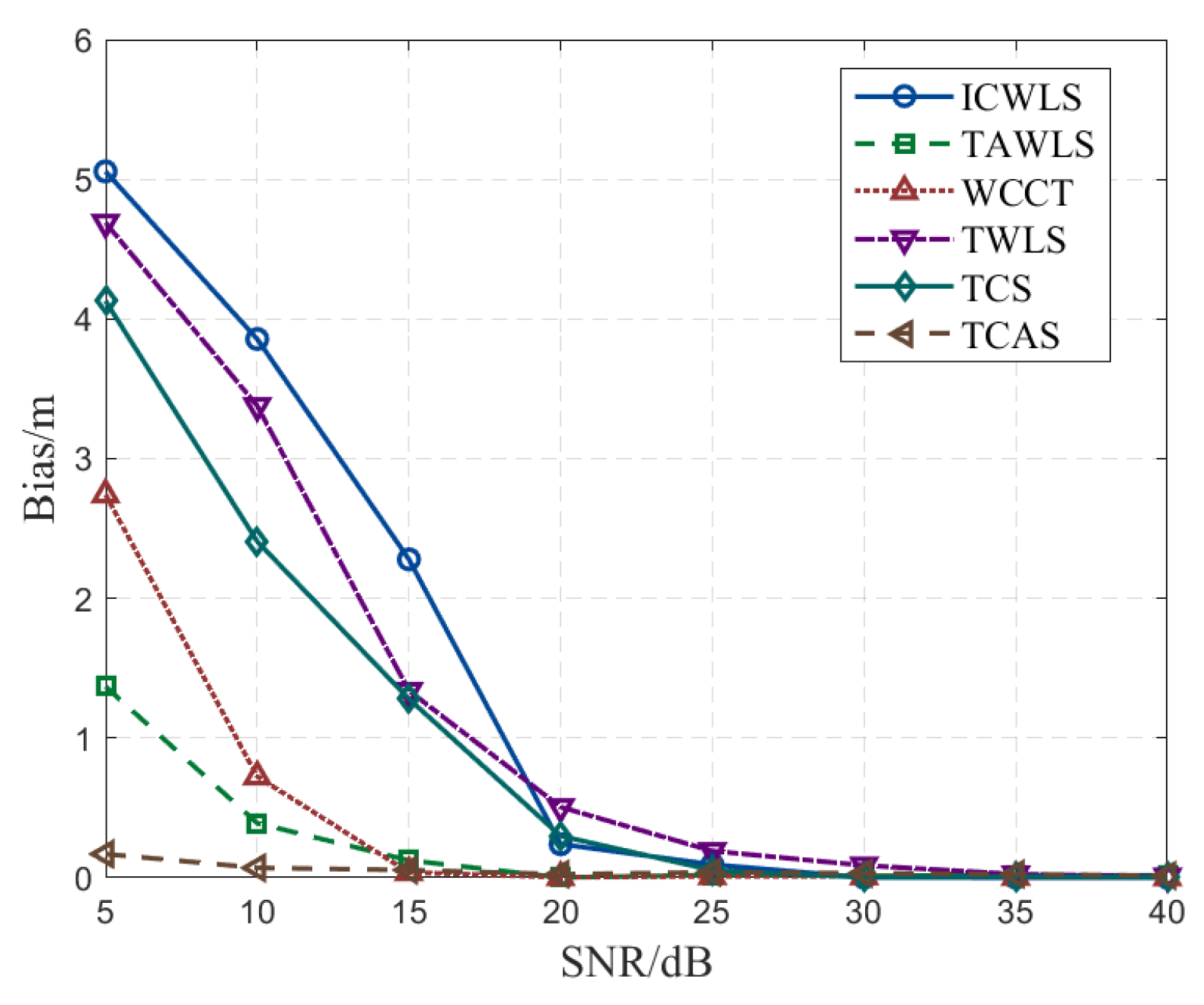
Figure 5 shows the positioning errors of each algorithm in the SNR range of 5–40 dB when ${\sigma }_{\phi }=1^o$. Under the condition of high SNR, all algorithms can achieve ideal positioning results. The convergence of the TWLS and ICWLS algorithms is weaker than that of the other algorithms. In the case of low SNR, the TAWLS algorithm and the TCAS algorithm of mixed AOA measurement information are obviously better than other algorithms.

Figure 6 illustrates the impact of AOA noise on the performance of the TAWLS and TCAS algorithms under different TDOA noise conditions. It can be seen from the figure that under different TDOA noise conditions, the deviation of the TCAS algorithm is significantly lower than that of the TAWLS algorithm. As AOA noise increases, the TCAS algorithm’s deviation remains below 0.2 m. For AOA noise, the TAWLS algorithm is more sensitive to the change in the TDOA noise, which has a greater impact on the estimation results. Therefore, the TCAS algorithm has better robustness in dealing with AOA noise when the TDOA noise is larger.

4.2. The Effect of the Number of Sensors on Algorithm Performance

In practical application scenarios, the sensor array constitutes the primary component for signal reception. Achieving optimal and consistent signal reception can often prove challenging. This is due to the signal being subject to interference by a number of factors in the propagation environment. These factors include the complex indoor environment, which can result in signal occlusion and reflection, and the receiver’s FOV. Simultaneously, to enhance the precision and dependability of the TAWLS and TCAS algorithms, a specific number of superfluous equations were incorporated. In an ideal environment, these redundant equations can have a positive impact; however, in the actual operating environment, the effect may be altered due to the poor signal received by the sensor and other factors, thus affecting the performance of the entire algorithm. In order to make the research more suitable for the conditions of practical application, the TCAS and TAWLS algorithms were tested with a different number of sensors.

The ${\sigma }_{\phi }$ was set to 1°, the SNR range of TDOA was set to 5–40 dB, and the number of sensors N was changed to conduct comparative experiments. The simulation parameters in this subsection remain the same as in the previous subsection. When selecting the PDs, ${\mathbf{p}}_1$ was fixed to be selected, because ${\mathbf{p}}_1$ is fixed to the top surface and generally receives the signal. We randomly selected $N-1$ PDs from the other four PDs for the experiment.

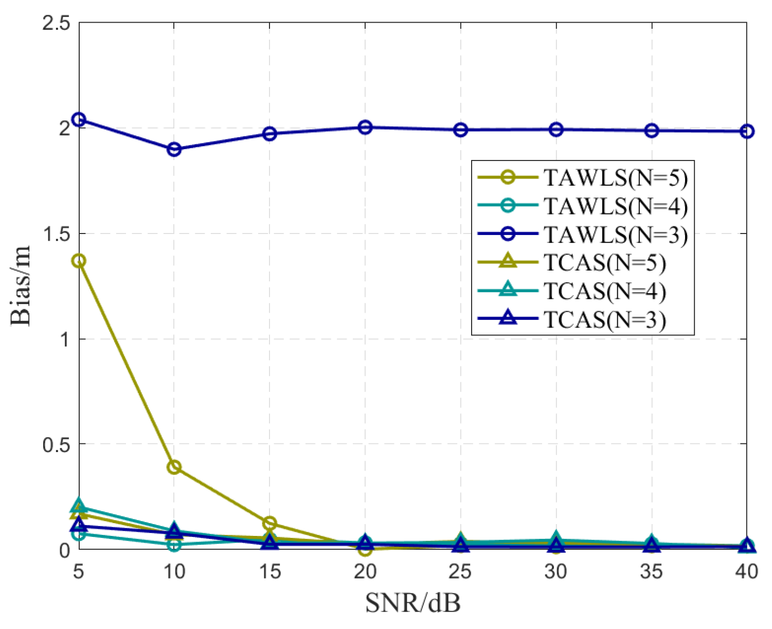
Figure 7 shows the effect of varying the number of PDs $N=3,4,5$ on the localization performance under different TDOA SNR conditions, comparing the proposed TCAS algorithm with the baseline TAWLS method. It can be observed that for TAWLS, the positioning error increases significantly as N decreases, especially under low SNR conditions. For example, when SNR = 5 dB, the bias of TAWLS rises from 1.4 m ($N=5$) to over 2.0 m ($N=3$), indicating strong dependence on TDOA measurement redundancy. In contrast, TCAS maintains a much more stable error across all values of N, and its performance remains nearly unchanged even when the number of sensors is reduced to three.

Interestingly, in low SNR environments, the localization error of TCAS slightly decreases as N decreases. This result is attributed to the increased relative influence of the AOA measurements when fewer PDs are used, as the number of TDOA constraints diminishes. Since the angular observation geometry remains consistent, TCAS shifts reliance toward the more stable AOA constraints, which helps suppress the impact of TDOA noise under sparse configurations.

4.3. Analysis of Overall Algorithm Performance

In order to verify the effectiveness of the proposed algorithm, we used the algorithms to localize the sources at different locations. We numerically simulated $10\times 10$ test points uniformly distributed in the 10 m × 10 m × 5 m region, where the coordinates of x and y ranged from 1 to 10, and coordinate z was fixed at 5. In the experiment, we localized the LEDs located at each of these 100 test points, we set the coordinates of ${\mathbf{p}}_1$ to be (0, 2, 0), and the coordinates of the other PDs were obtained from Table 2. Also, we assume here that the signal of each test point can be received by all PDs. The bias was used in the experimental results to indicate the performance of the algorithms. 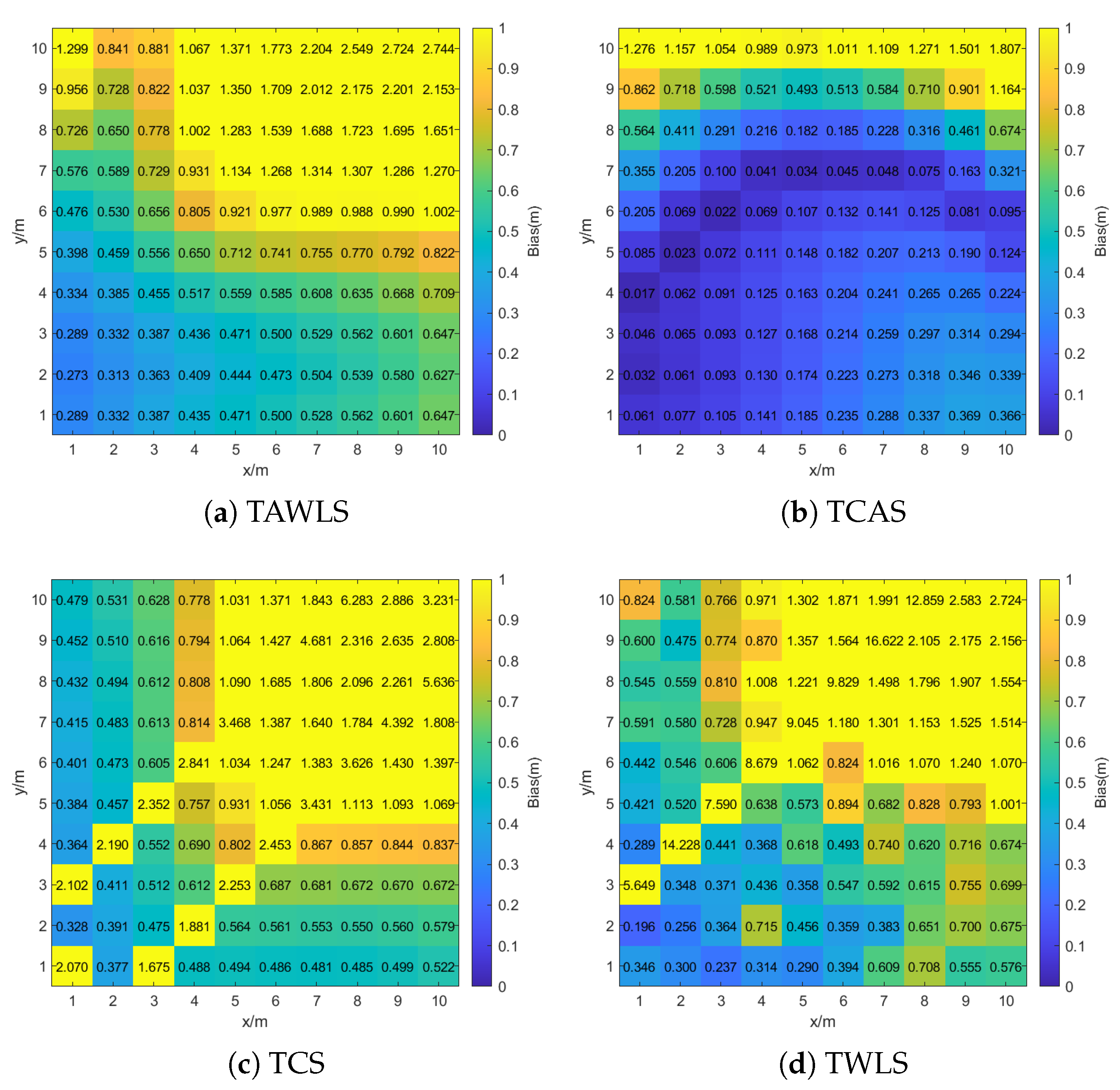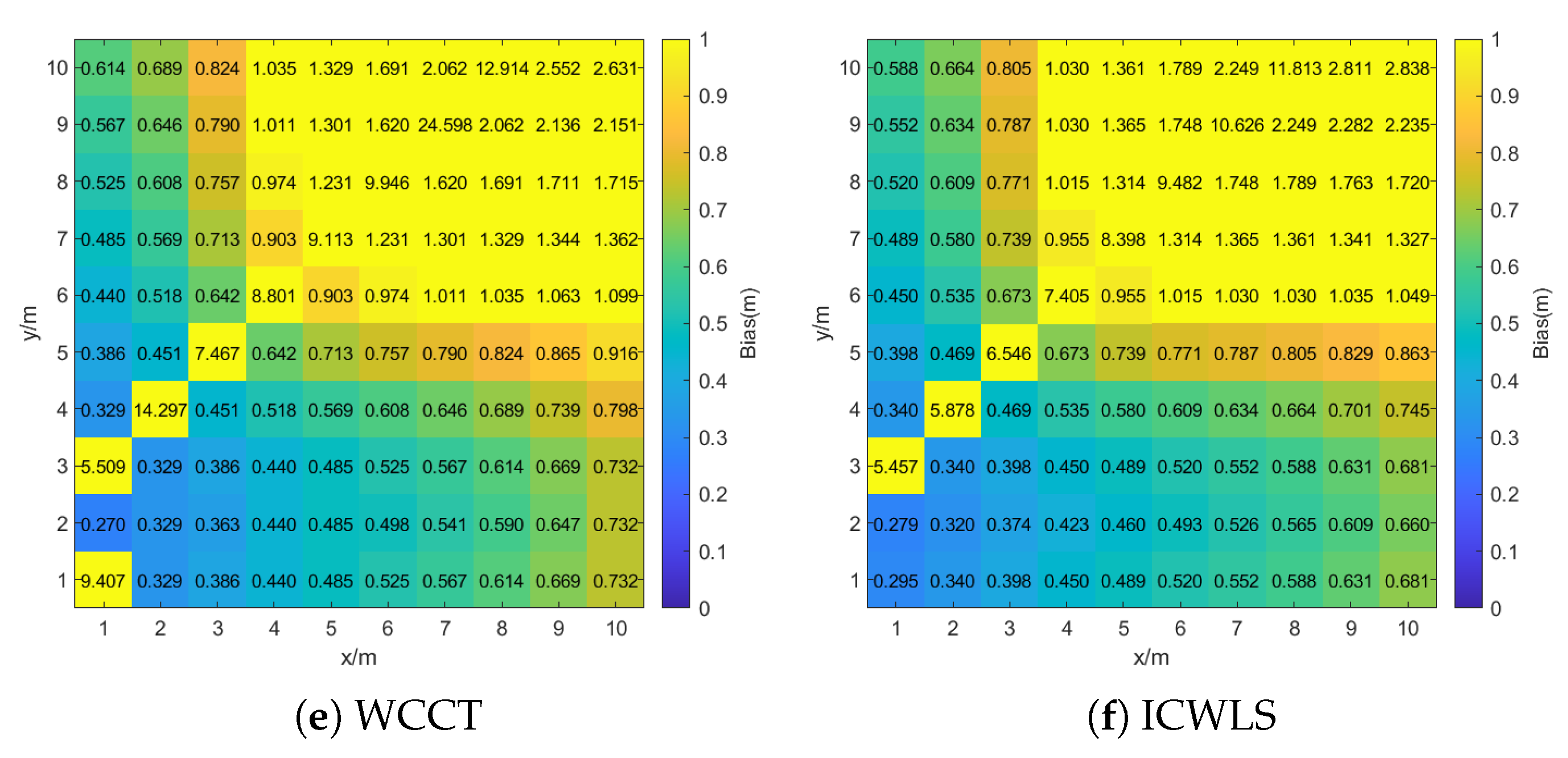We set SNR = 20 dB and ${\sigma }_{\phi }=1°$, and the positioning coordinates of different positioning algorithms were compared with the actual coordinates, as shown in Figure 8.

Figure 8 shows the spatial distribution of the localization bias across the indoor region. It can be observed that most baseline algorithms, such as TAWLS, TCS, TWLS, WCCT, and ICWLS, exhibit larger positioning errors near the upper-right corner of the room (e.g., when $x\ge 8$), with some errors exceeding 2.5 m. This is primarily due to the degradation of TDOA geometric diversity and increased noise in regions farther from the PD array.

Interestingly, it is also observed that in certain points close to the PD array, TDOA-only methods (TCS, TWLS, WCCT and ICWLS) still show unexpectedly large errors. This is attributed to geometric degeneration, where the distances from multiple PDs to the LED source become nearly equal. In such cases, the time difference of arrival becomes approximately the same, leading to poor sensitivity and poor localization results.

In contrast, the proposed TCAS algorithm maintains consistently low errors across the room. Most locations have errors below 0.2 m. This highlights the robustness and adaptability of TCAS, which combines both TDOA and AOA information and is optimized using semidefinite relaxation to mitigate noise and geometric limitations.

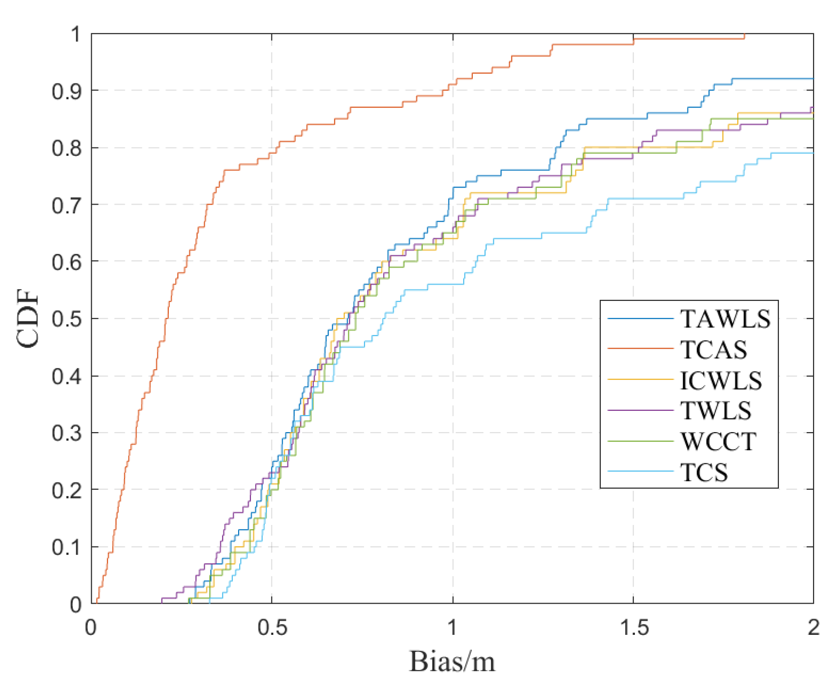
The superior performance of the TCAS algorithm is further illustrated in Figure 9, which uses a biased cumulative distribution function (CDF) to evaluate the performance of the TCAS algorithm and other algorithms.

Figure 9 shows the CDF of the various algorithm deviations. In general, 70% of the localization errors obtained by the TCAS algorithm are below 0.25 m, which indicates that most of the positioning errors are closely clustered near the low value. In contrast, traditional algorithms such as ICWLS and TWLS show significantly poor performance, reflecting their sensitivity to measurement noise. Furthermore, compared to the TAWLS algorithm, the TCAS algorithm has a more pronounced upward trend, especially in the low deviation range that is critical for high-precision applications.

To provide a more comprehensive comparison among the studied localization algorithms, we further analyzed their computational complexity.

Figure 10 presents the average computation time of each algorithm under identical simulation settings. As shown, WCCT and TWLS achieve the lowest runtime, with average delays below 6 ms, making them suitable for fast response scenarios. ICWLS and TAWLS require moderate computation time, while the proposed TCAS algorithm incurs the highest cost, averaging approximately 17 ms. The overall computation time remains within a reasonable range for near-real-time indoor localization. This increase is mainly due to the SDR formulation and the joint utilization of TDOA and AOA information, which adds computational complexity but significantly enhances the robustness and accuracy.

To further interpret the performance gains shown in Figure 8 and Figure 9, we analyzed the fundamental mechanisms that contribute to the superiority of the proposed TCAS algorithm compared with the baseline methods.

First, TCAS jointly utilizes TDOA and AOA measurements, which provide complementary spatial information. TDOA is sensitive to timing accuracy and geometry, whereas AOA is more robust to certain noise types and less dependent on distance. By integrating these two sources, TCAS significantly improves the estimation stability, especially in challenging scenarios such as geometrically degenerate regions or low SNR conditions.

Second, the localization problem in TCAS is formulated as a convex SDP task through SDR. Unlike traditional least-squares approaches that may fall into local minima or suffer from poor conditioning, this convex formulation ensures global optimization, greater numerical stability, and reduced sensitivity to initial values and measurement variance.

Third, TCAS also incorporates symmetry-aware modeling of AOA paths. This additional geometric exploitation allows the algorithm to better utilize angular constraints, further enhancing the robustness.

These algorithmic innovations explain the consistent improvement observed in both mean error and maximum error metrics across the spatial domain. In summary, the combination of multi-modal fusion, convex optimization, and structured geometric modeling forms the foundation of TCAS’s superior performance over conventional localization methods.

Although this study primarily focuses on simulation-based validation, we acknowledge the importance of physical experimentation in evaluating real-world performance. At present, the practical implementation of IRS in visible light systems is still at an early stage, especially regarding controllable reflection direction and optical specular stability. In addition, accurate synchronization and angle sensing required for joint TDOA and AOA measurements involve hardware modules that are still under development. Future work will focus on system prototyping, calibration, and performance testing under dynamic conditions to facilitate practical deployment.

5. Conclusions

In this paper, a novel visible light indoor positioning method combined with IRS is proposed. This method is intended to improve the positioning accuracy and stability in complex environments by introducing the concepts of a virtual signal source and virtual receiver. The experimental results demonstrate that the proposed method exhibits excellent positioning performance under various SNR and sensor configurations. Compared to traditional methods, this approach significantly reduces the positioning error. Although the proposed method has achieved remarkable results in improving the positioning accuracy and stability, the limitations of SDP, the computational cost, and the challenges of IRS deployment still need to be further studied and solved. Future work will be dedicated to optimizing these aspects to promote the further development of high-precision indoor positioning technology.

References

1. Singh, J.; Tyagi, N.; Singh, S.; Ali, F.; Kwak, D. A Systematic Review of Contemporary Indoor Positioning Systems: Taxonomy, Techniques, and Algorithms. IEEE Internet Things J. 2024, 11, 34717–34733. [Google Scholar] [CrossRef]
2. Farahsari, P.S.; Farahzadi, A.; Rezazadeh, J.; Bagheri, A. A Survey on Indoor Positioning Systems for IoT-Based Applications. IEEE Internet Things J. 2022, 9, 7680–7699. [Google Scholar] [CrossRef]
3. Zafari, F.; Gkelias, A.; Leung, K.K. A Survey of Indoor Localization Systems and Technologies. IEEE Commun. Surv. Tutorials 2019, 21, 2568–2599. [Google Scholar] [CrossRef]
4. Abbas, M.; Elhamshary, M.; Rizk, H.; Torki, M.; Youssef, M. WiDeep: WiFi-based Accurate and Robust Indoor Localization System using Deep Learning. In Proceedings of the 2019 IEEE International Conference on Pervasive Computing and Communications (PerCom), Kyoto, Japan, 11–15 March 2019; pp. 1–10. [Google Scholar] [CrossRef]
5. Bastiaens, S.; Alijani, M.; Joseph, W.; Plets, D. Visible Light Positioning as a Next-Generation Indoor Positioning Technology: A Tutorial. IEEE Commun. Surv. Tutorials 2024, 26, 2867–2913. [Google Scholar] [CrossRef]
6. Chen, L.; Feng, L.; Wang, J.; Zhang, T.; Zhang, H.; Xue, Z. Hybrid Indoor Positioning System Based on LED Array. IEEE Photonics J. 2025, 17, 1–11. [Google Scholar] [CrossRef]
7. Liu, A.; Wang, W. An Indoor Positioning Method Based on Smartphone and Surveillance Camera. IEEE Sens. J. 2023, 23, 22742–22753. [Google Scholar] [CrossRef]
8. Zhang, K.; Zhang, Z.; Zhu, B. Beacon LED Coordinates Estimator for Easy Deployment of Visible Light Positioning Systems. IEEE Trans. Wirel. Commun. 2022, 21, 10208–10223. [Google Scholar] [CrossRef]
9. Amsters, R.; Demeester, E.; Slaets, P.; Holm, D.; Joly, J.; Stevens, N. Towards Automated Calibration of Visible Light Positioning Systems. In Proceedings of the 2019 International Conference on Indoor Positioning and Indoor Navigation (IPIN), Pisa, Italy, 30 September–3 October 2019; pp. 1–8. [Google Scholar] [CrossRef]
10. Ye, H.; Yang, B.; Long, Z.; Dai, C. A Method of Indoor Positioning by Signal Fitting and PDDA Algorithm Using BLE AOA Device. IEEE Sens. J. 2022, 22, 7877–7887. [Google Scholar] [CrossRef]
11. Terças, L.; Alves, H.; de Lima, C.H.M.; Juntti, M. Bayesian-Based Indoor Factory Positioning Using AOA, TDOA, and Hybrid Measurements. IEEE Internet Things J. 2024, 11, 21620–21631. [Google Scholar] [CrossRef]
12. Liu, C.; Zhang, Y. 5G Reconfigurable Intelligent Surface TDOA Localization Algorithm. Electronics 2024, 13, 2409. [Google Scholar] [CrossRef]
13. Feng, R.; Zhang, Z.; Lai, Z.; Mao, X. Time-difference-of-arrival positioning based on visible light communication for harbor-border inspection. Appl. Opt. 2022, 61, 8833–8842. [Google Scholar] [CrossRef]
14. Cong, L.; Zhuang, W. Hybrid TDOA/AOA mobile user location for wideband CDMA cellular systems. IEEE Trans. Wirel. Commun. 2002, 1, 439–447. [Google Scholar] [CrossRef]
15. Badriasl, L.; Kennedy, H.; Finn, A. Effects of coordinate system rotation on two novel closed-from localization estimators using azimuth/elevation. In Proceedings of the 16th International Conference on Information Fusion, Montbeliard, France, 28–31 October 2013; pp. 1797–1804. [Google Scholar]
16. Yin, J.; Wan, Q.; Yang, S.; Ho, K.C. A Simple and Accurate TDOA-AOA Localization Method Using Two Stations. IEEE Signal Process. Lett. 2016, 23, 144–148. [Google Scholar] [CrossRef]
17. Jia, T.; Wang, H.; Shen, X.; Jiang, Z.; He, K. Target localization based on structured total least squares with hybrid TDOA-AOA measurements. Signal Process. 2018, 143, 211–221. [Google Scholar] [CrossRef]
18. Kang, X.; Wang, D.; Shao, Y.; Ma, M.; Zhang, T. An Efficient Hybrid Multi-Station TDOA and Single-Station AOA Localization Method. IEEE Trans. Wirel. Commun. 2023, 22, 5657–5670. [Google Scholar] [CrossRef]
19. Ho, K.C. Bias Reduction for an Explicit Solution of Source Localization Using TDOA. IEEE Trans. Signal Process. 2012, 60, 2101–2114. [Google Scholar] [CrossRef]
20. Wang, G.; Ho, K.C. Convex Relaxation Methods for Unified Near-Field and Far-Field TDOA-Based Localization. IEEE Trans. Wirel. Commun. 2019, 18, 2346–2360. [Google Scholar] [CrossRef]
21. Yang, L.; Gao, H.; Ling, Y.; Zhou, S.; Li, B. 3D Joint Estimation of Position and Velocity for a Moving Target in Multistatic Radar System by VHC-2WLS Algorithm. IEEE Commun. Lett. 2020, 24, 1939–1943. [Google Scholar] [CrossRef]
22. Zhang, L.; Zhang, T.; Shin, H.S. An Efficient Constrained Weighted Least Squares Method with Bias Reduction for TDOA-Based Localization. IEEE Sens. J. 2021, 21, 10122–10131. [Google Scholar] [CrossRef]
23. Wang, S.; He, Y.; Yin, B.; Ning, S.; Zeng, W. Partial Discharge Localization in Substations Using a Regularization Method. IEEE Trans. Power Deliv. 2021, 36, 822–830. [Google Scholar] [CrossRef]
24. Sun, S.; Yang, F.; Song, J.; Han, Z. Joint Resource Management for Intelligent Reflecting Surface–Aided Visible Light Communications. IEEE Trans. Wirel. Commun. 2022, 21, 6508–6522. [Google Scholar] [CrossRef]
25. Zhang, H.; Di, B.; Song, L.; Han, Z. Reconfigurable Intelligent Surfaces Assisted Communications with Limited Phase Shifts: How Many Phase Shifts Are Enough? IEEE Trans. Veh. Technol. 2020, 69, 4498–4502. [Google Scholar] [CrossRef]
26. Zhang, G.; Zhang, D.; Deng, H.; Wu, Y.; Zhan, F.; Chen, Y. Practical Passive Indoor Localization with Intelligent Reflecting Surface. IEEE Trans. Mob. Comput. 2024, 23, 12477–12490. [Google Scholar] [CrossRef]
27. Abdelhady, A.M.; Salem, A.K.S.; Amin, O.; Shihada, B.; Alouini, M.S. Visible Light Communications via Intelligent Reflecting Surfaces: Metasurfaces vs. Mirror Arrays. IEEE Open J. Commun. Soc. 2021, 2, 1–20. [Google Scholar] [CrossRef]
28. Ohyama, T.; Kawamoto, Y.; Kato, N. Standalone Intelligent Reflecting Surface with Automatic Update of Phase-Shift Switching Schedule for Improved Communication and Localization. IEEE Trans. Veh. Technol. 2024, 73, 8503–8513. [Google Scholar] [CrossRef]
29. Kokdogan, F.; Gezici, S. Intelligent Reflecting Surfaces for Visible Light Positioning Based on Received Power Measurements. IEEE Trans. Veh. Technol. 2024, 73, 13108–13121. [Google Scholar] [CrossRef]
30. Tang, W.; Chen, M.Z.; Chen, X.; Dai, J.Y.; Han, Y.; Di Renzo, M.; Zeng, Y.; Jin, S.; Cheng, Q.; Cui, T.J. Wireless Communications with Reconfigurable Intelligent Surface: Path Loss Modeling and Experimental Measurement. IEEE Trans. Wirel. Commun. 2021, 20, 421–439. [Google Scholar] [CrossRef]
Figure 1. Channel model using PD to receive LOS and IRS-reflected signals.
Electronics 14 02158 g001
Figure 2. Virtual paths model.
Electronics 14 02158 g002
Figure 3. IRS rotates around the x and z axes.
Electronics 14 02158 g003
Figure 4. Sensor array structure.
Electronics 14 02158 g004
Figure 5. Average localization error under varying SNR conditions.
Electronics 14 02158 g005
Figure 6. Performance of the source localization as σ φ increases.
Electronics 14 02158 g006
Figure 7. Localization error comparison under different TDOA SNRs with varying numbers of PDs.
Electronics 14 02158 g007
Figure 8. The positioning error of each algorithm when locating signal source at different positions.
Electronics 14 02158 g008aElectronics 14 02158 g008b
Figure 9. CDF of biases for different algorithms.
Electronics 14 02158 g009
Figure 10. Comparison of computational complexity for different algorithms.
Electronics 14 02158 g010