Optimized Universal Droop Control Framework for Enhancing Stability and Resilience in Renewable-Dense Power Grids

Abstract

High penetration of green energy sources presents substantial challenges to grid stability and resilience, primarily due to inherent voltage and frequency variability, which worsens during critical events. This study proposes an integrated framework for stability and resilience enhancement in renewable-dense power grids by designing optimized universal droop controllers (UDCs) tailored for grid-forming operations under high-impact contingencies. The UDC incorporates fault localization functionality via grid-forming inverters embedded with phasor measuring capabilities (phase voltage magnitude and angle) to facilitate real-time fault detection and response, thus augmenting operational reliability. Leveraging integrated solution environments, the developed framework employs numerical optimization routines for resource allocation, load prioritization, economic dispatch of distributed energy resources (DERs), and adaptive network reconfiguration under constrained conditions and during critical events that may necessitate decentralized network configurations in the wake of main grid failures. Validation conducted on the IEEE 123-node distribution network indicates that the optimized UDC framework achieves superior voltage and frequency regulation compared to conventional droop-based methods, ensuring optimal resource distribution and sustained load support.

1. Introduction

The growing integration of distributed energy resources into the power grid is essential in achieving sustainable energy goals but introduces new challenges for grid stability and reliability. DERs, like wind and solar, are not consistent in supply, leading to fluctuations in power generation that can destabilize voltage and frequency levels. As the global energy landscape shifts toward increased decentralization, there is an urgent need for microgrid solutions that can maintain stability and ensure efficient power sharing, even under variable and challenging operating conditions. Traditional control methods, like the widely adopted droop control strategy, provide a basis for decentralized power sharing but have limitations when applied to complex microgrid configurations, particularly in island operations where communication links are minimal or absent. These challenges can be further amplified during extreme events such as hurricanes, flooding, and severe snowstorms that can disrupt main grid connections, necessitating robust, standalone control within microgrids.

Recent advancements in decentralized control strategies have enhanced droop control for microgrids, improving stability and accuracy in power-sharing under variable loads and mismatched impedances. Dual-frequency droop control (DFDC) addresses these challenges by adjusting power-sharing based on local frequency changes, distributing real, reactive, and harmonic powers precisely without relying on communication links. Additionally, incorporating a dynamic droop slope regulator (DDR) mitigates frequency deviations, thus stabilizing distributed generation (DG) units [1,2,3,4,5]. Dynamic nonlinear droop control (DNDC) further improves power-sharing by introducing nonlinear gain adjustments, which has hardware testing validated as effective under heavy loads, outperforming traditional methods [6,7,8,9,10].

Advanced droop control (ADC) refines droop control by focusing on reactive power sharing to stabilize voltage levels, especially in islanded microgrids. ADC minimizes reactive power-sharing errors, enhancing renewable integration, and balancing voltage under dynamic conditions [11,12,13,14,15]. Similarly, adaptive droop control enables flexible power limits and current adjustments in response to grid disturbances [16]. This adaptive control method improves power quality and prevents overloading by dynamically controlling output, enhancing microgrid resilience against faults. In addition, adaptive hierarchical and consensus-based controls add flexibility by supporting transitions between master–slave and peer-to-peer modes for more effective power-sharing [17,18,19,20].

Adaptive droop control (ADC) enables gain modulation based on system dynamics. While ADC enhances regulation precision, reducing steady-state errors from over 5% to approximately 4.2%, its real-time implementation requires substantial computation, limiting responsiveness in rapidly changing environments [21]. UDC provides a low-latency response (<200 ms), enhanced regulation accuracy (<1.5% steady-state error), and improves power-sharing efficiency by up to 18% compared to ADC. Quantitative performance comparisons under IEEE 14-bus test scenarios indicate that UDC outperforms ADC and DFDC in load disturbance rejection by 30%, achieves a 25% faster recovery time under voltage sag events, and ensures optimal power flow with less than 1.2% variance from centralized dispatch [22,23].

In grid-connected applications, droop control with current-limiting features helps DG control units to manage grid fluctuations more effectively. For instance, droop control with floating characteristics stabilizes power and current for inverter-based DG units, handling frequency, and voltage fluctuations to improve power quality [24,25,26]. Offshore wind farms also benefit from droop control through DC link current controllers that enhance stability and operational efficiency, even during faults or varying wind speeds, supporting HVDC transmission integration [7]. Multi-terminal HVDC systems in hybrid AC/DC networks employ adaptive droop techniques to dynamically adjust droop coefficients, thus reducing transient overshoot and enhancing frequency and voltage stability with lead-lag compensators [8,18,27].

In DC microgrids, the adaptive master–slave (AMS) control strategy uses nonlinear droop controllers for seamless control mode transitions and improved power-sharing among voltage source converters (VSCs). This approach ensures coordinated power sharing in multi-terminal systems under changing grid conditions and during contingencies, such as converter outages or shifts in renewable output [3,13,19,25]. Optimization based on multiple objectives, like the nondominated sorting genetic algorithm II (NSGA II), has been applied to droop-controlled systems, enhancing voltage regulation, reducing losses, and improving current sharing by using fuzzy logic for control evaluation under conflicting objectives [14,24].

Despite these advancements, challenges persist in decentralized microgrid control. While DFDC [1,2,3] and DNDC [6,8] facilitate communication-free power sharing, achieving precise voltage and frequency control under variable conditions remains difficult. Approaches like ADC [11,13] and adaptive droop control [12,19,20] enhance reactive power sharing and current limiting but still face challenges under extreme conditions, such as fault events or severe weather. Additionally, adaptive droop methods in applications like multi-terminal HVDC [18,25] and DG optimization [19,24] improve efficiency but often lack the dynamic resource management needed for high-stakes, resource-limited conditions. As microgrids evolve, developing robust solutions to address these gaps will be essential.

The proposed work addresses these gaps by introducing a universal droop controller (UDC) in grid-forming mode, designed to enhance both precision and resilience in microgrid control. Unlike prior methods, the UDC integrates GAMS-enabled optimization to maximize load and resource allocation dynamically, ensuring efficient economic dispatch across DERs. Additionally, the UDC incorporates fault localization capabilities by using grid-forming inverters with PMU functionalities, which enable real-time fault detection and response. This approach not only achieves high precision in voltage and frequency control, but also supports resilient, autonomous operation during low-frequency, high-impact events, fulfilling key requirements for modern, reliable microgrids as resiliency-enhancing tools [28,29]. Summarized below are the major contributions of the proposed model:

• Achieving better voltage/frequency control under varied line conditions;
• Integrating frameworks for load and resource allocation across multiple DERs;
• Integrating a grid-forming inverter with phasor measuring capabilities for real-time network monitoring and fault detection to ensure network stability;
• Maintaining autonomous operation (resilient) during high-impact disruptions (loss of distribution line, loads, and DERs);
• Supporting stable performance in both grid-tied and islanded microgrids.

The GAMS-UDC approach offers several novel features compared to existing methods like DFDC, DNDC, or ADC. First, it leverages GAMS for numerical optimization, providing efficient and timely power system management that surpasses heuristic methods. The GAMS-UDC approach operates without communication protocols, relying solely on local variables for control, which enhances system reliability and reduces complexity. Unlike metaheuristic approaches such as HHO, the GAMS-UDC approach is problem-dependent, offering more realistic and effective solutions tailored to the specific characteristics of the system. It also provides a robust and adaptable solution across multiple microgrids, accommodating various power system configurations. The approach reduces operational and resource dispatch costs by using optimization, leading to lower implementation costs. Additionally, it achieves fast network reconfiguration (within 200 milliseconds) during high-impact low-frequency (HILF) events. Finally, GAMS optimization significantly reduces simulation time, delivering optimal solutions efficiently when the model is properly implemented.

The rest of the paper is organized as follows: Section 2 presents the materials and methods, mathematical modeling, and GAMS optimization modeling. A case study considering different fault conditions and load scenarios is presented in Section 3. Relevant results are also reported in Section 3. Section 4 further discusses the results and Section 5 concludes our work. Finally, Appendix A presents important distribution network configuration resources.

2. Materials and Methods

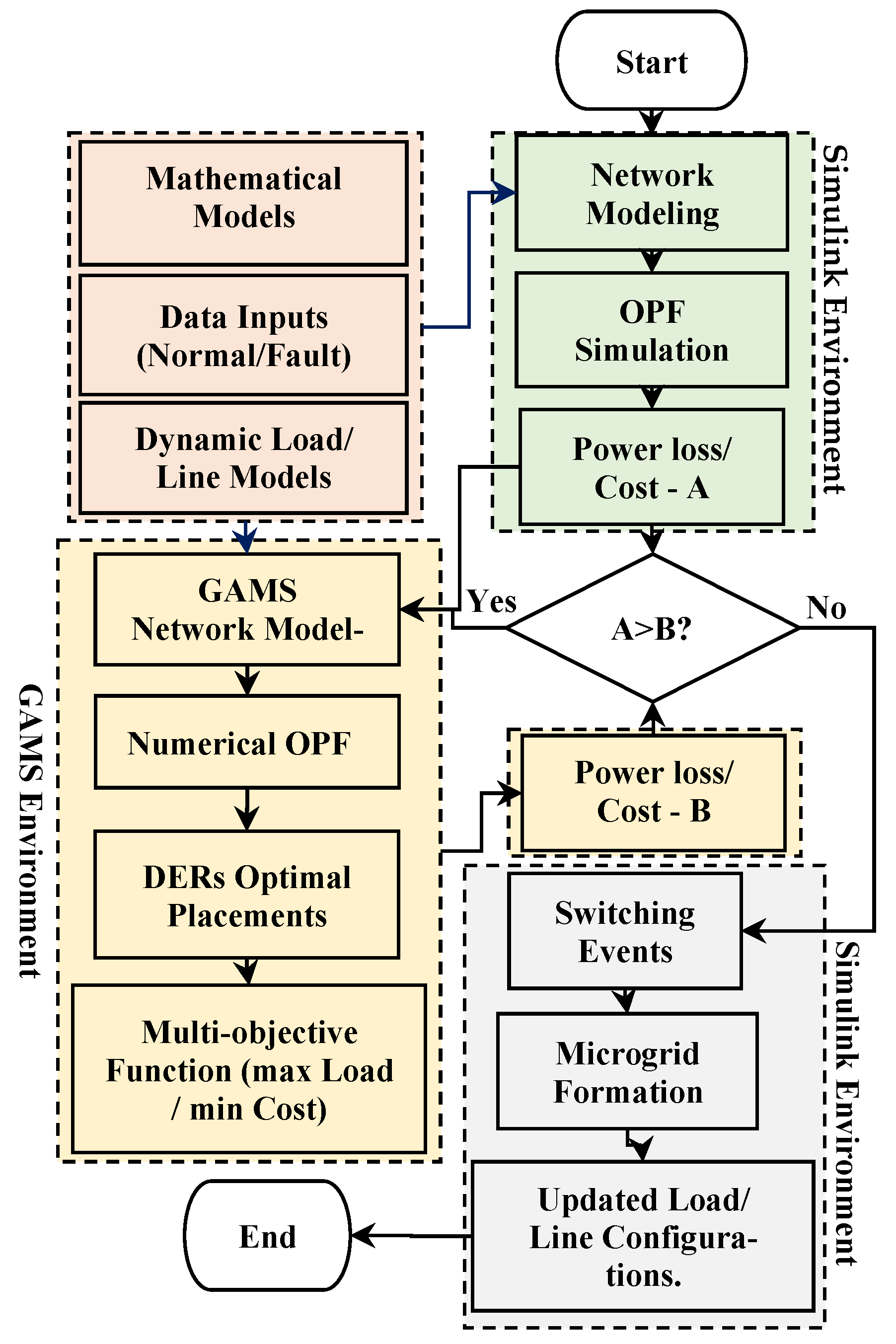
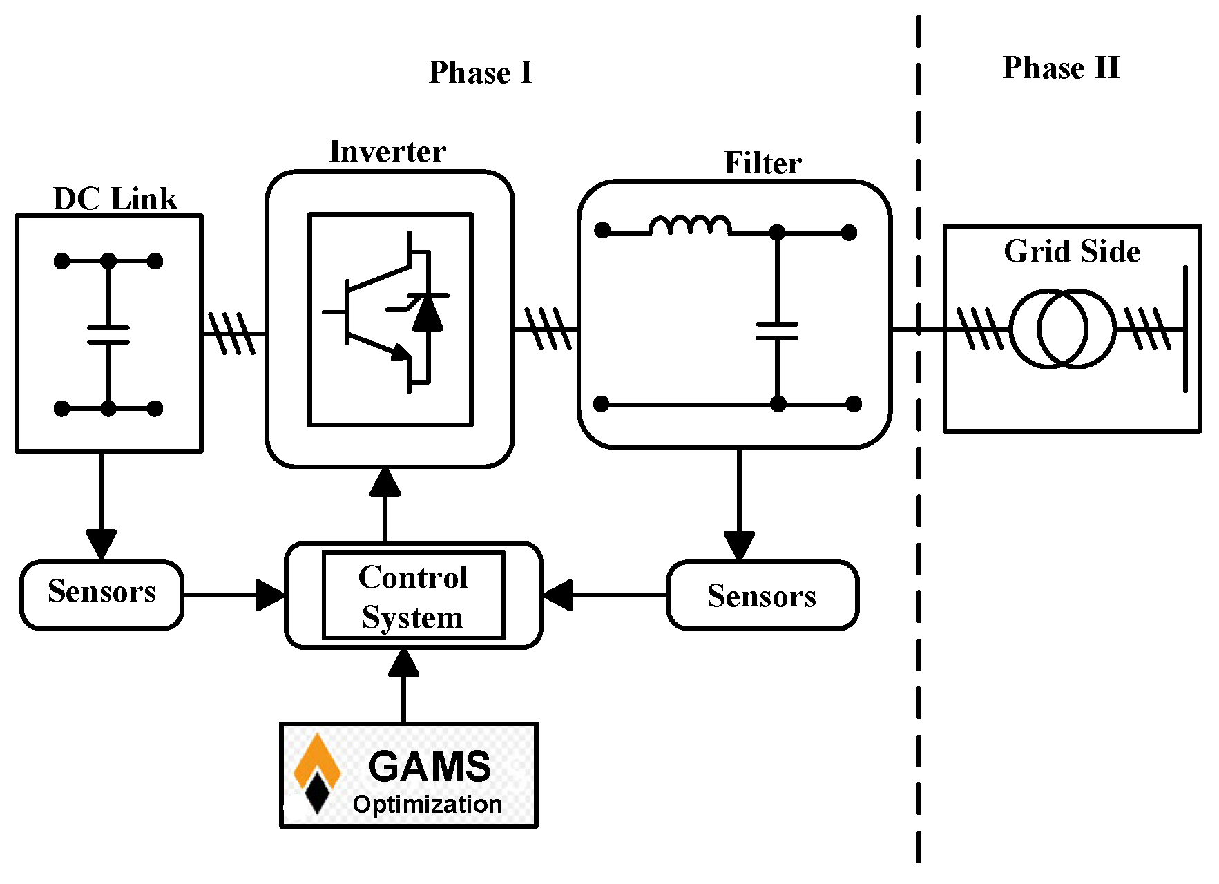
Proposed Integrated Framework

The proposed framework is shown in Figure 1, depicting the step-by-step procedures for implementing the integrated solution for grid stability and resilience enhancement.

The optimization model is divided into two parts, namely, (i) MATLAB R2023a MATLAB-Simulink electrical network modeling and (ii) GAMS 43.4.0 numerical optimization. A seamless data exchange is established between the electrical network model in Simulink and the GAMS environment through the MATLAB workspace and Excel file. MATLAB-Simulink simulates the power flow of the unbalanced three-phase of the modeled network. The electrical network consists of multiple DERs that are inverter-based with grid-forming GF-UDC controllers. The Simulink model of the electrical network incorporates four UDCs in the grid-forming inverters provisioned with systemic parametric variables tuning using an enhanced system transfer function. Figure 2a shows the GF-UDC that self-synchronizes with the grid.

The inverter’s current-limiting capability is implemented through software control (algorithm), which operates based on the outer and firing control loops. These loops, as shown in Figure 2b, incorporate GAMS numerical optimization to determine reference values for generating firing signals within the current control block. The load’s active and reactive power controls are optimized via GAMS and provide inputs to the supplementary and outer control loops, effectively constraining the current drawn from the inverters. The active power controller stabilizes the inverter’s voltage output by adjusting voltage differences between the grid and the inverter. GF-UDC enables voltage and frequency management in island modes, improving power system stability. On the other hand, GAMS performs the numerical optimization of the simulated electrical network using a mixed-integer linear programming (MINLP) solver (SCIP) and a Mixed Integer Programming (MIP) solver (CPLEX). The MINLP and MIP solvers handle OPF analysis, DER allocation, generation cost minimization, load management, load curtailment, switching operations, and microgrid formation. This is a two-layer operation. The Simulink model calls the optimized DERs and switches from GAMS, streamlining integration and improving network stability and resilience while reducing simulation convergence time.

The integrated solution framework flow chart is presented in Figure 3. The design framework in Figure 3 includes several key components: first, a robust grid-forming inverter (GFI) implemented to enhance grid resilience by minimizing active power oscillations throughout the network. Second, dynamic load control mechanisms are employed to adaptively manage loads based on available resources and system constraints.

Third, microgrid formation is guided by GAMS optimization outputs, aligning with specified objective functions and constraints to ensure resilient operation. Finally, optimized switch control is incorporated to maximize load in cases of main grid failures, distribution line disruptions, or DER losses. Figure 4 illustrates the typical import of GAMS numerical optimization on the inverter UDC control mechanism in limiting the current drawn from the inverter per unit of time.

3. Mathematical Modeling

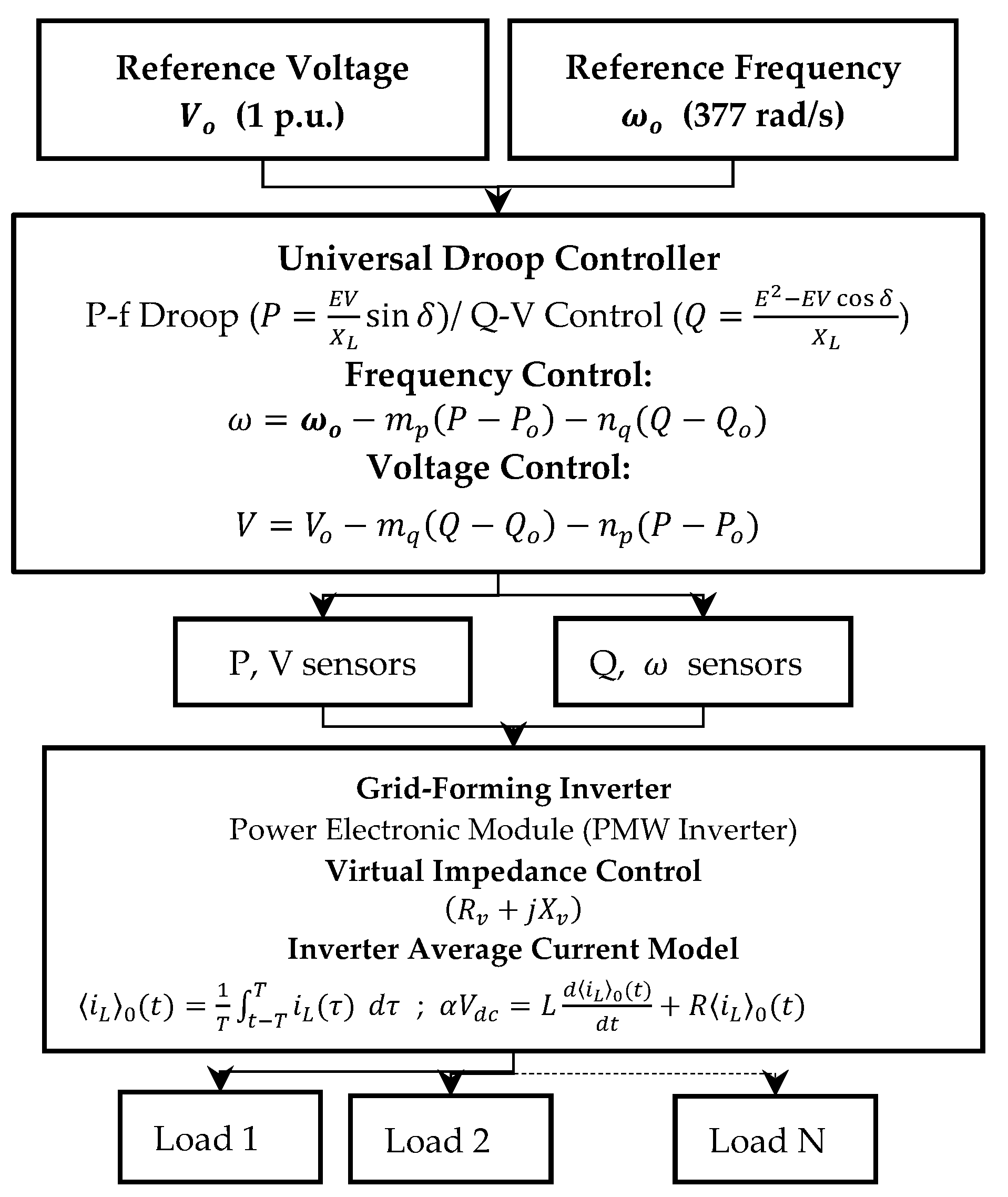
3.1. Grid-Forming Universal Droop Controller (GFM-UDC)

Designing a universal droop controller (UDC) with both frequency and voltage control is a core task in decentralized control of inverter-based distributed energy resources (DERs), especially in microgrids. UDC is a generalized droop control strategy that regulates both frequency via active power (P) and voltage via reactive power (Q). It combines P–f droop, which adjusts frequency based on active power output, and Q–V droop to adjust voltage based on reactive power. It also includes secondary control loops to eliminate steady-state error and adapt to grid dynamics. To achieve autonomous microgrid inverter control in island mode, with grid-forming capability and no communication, there is need to design local control laws based entirely on local power network measurements. The integration of general algebraic modeling system (GAMS) numerical optimization in the control mechanism design, as shown in Figure 4 above, further enhances the UDC accuracy, resilience, and robustness in managing several network contingencies. The equations describing the modeling of the proposed GFM-UDC are presented in Section 3.1.1.

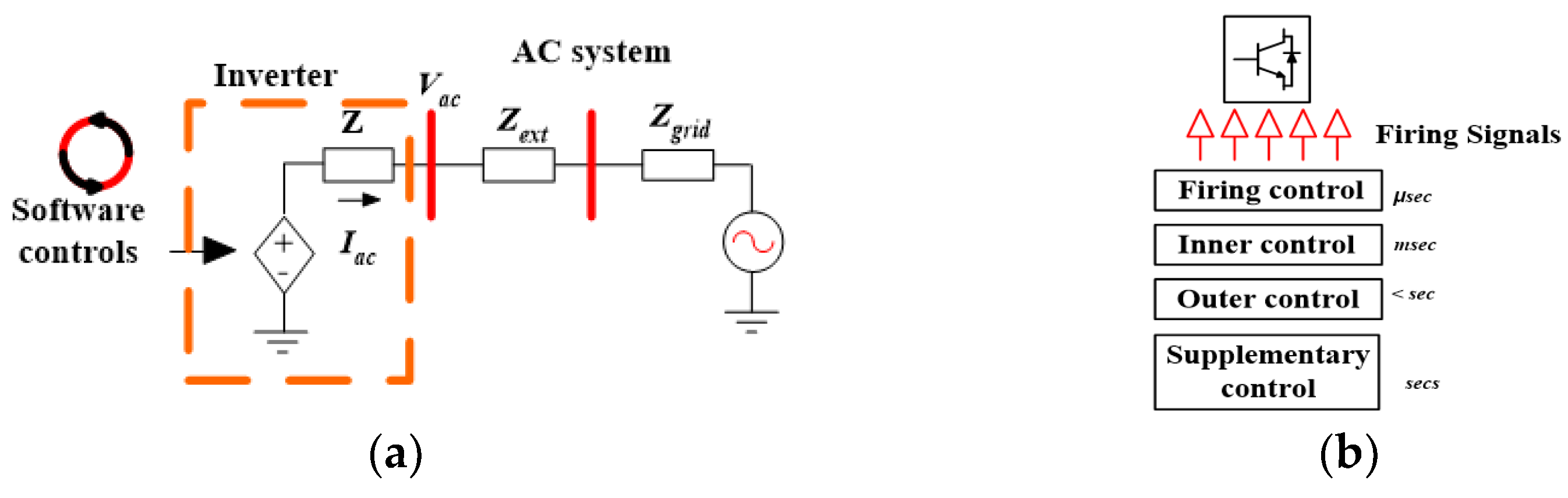
3.1.1. Dynamic Modeling of Droop Control with Inverter

The four inverter dynamics have been incorporated using a first-order filter, as shown in Equations (1)–(32). The active and reactive power dynamics for each inverter are given in Equations (1) and (2), respectively.

$${\tau }_P{\displaystyle \frac{d{P}_i}{dt}}+P_i=P_{ref,i} \forall i\in \left\{N\right\}$$

(1)

$${\tau }_Q{\displaystyle \frac{d{Q}_i}{dt}}+Q_i=Q_{ref,i} \forall i\in \left\{N\right\}$$

(2)

where $P_{ref,i}$ and $Q_{ref,i}$ are the nominal/reference/scheduled active and reactive power derived using the frequency and voltage droop control in Equations (3) and (4), respectively, ${\tau }_P$ and ${\tau }_Q$ are active and reactive power time constants, and $N$ is a set of inverters.

$$f=f_{ref,i}-K_P\left(P_i-P_{ref,i}\right) \forall i\in \left\{N\right\},$$

(3)

$$V=V_{ref,i}-K_Q\left(Q_i-Q_{ref,i}\right) \forall i\in \left\{N\right\}$$

(4)

where $f_{ref,i}$ and $V_{ref,i}$ are the nominal/reference frequency and voltage, $P_i$ and $Q_i$ are the measured output active and reactive power, and $K_P$ and $K_Q$ are the frequency and voltage droop coefficients, respectively. Equations (1)–(4) can be re-expressed in state-space model form as shown by Equation (16). Power dynamics to incorporate inverter filtering and response delay are given in Equations (5) and (6), respectively.

$${\tau }_P{\displaystyle \frac{d{P}_i}{dt}}+P_i=P_{meas, i}\forall i\in \left\{N\right\},$$

(5)

$${\tau }_Q{\displaystyle \frac{d{Q}_i}{dt}}+Q_i=Q_{meas, i}\forall i\in \left\{N\right\},$$

(6)

where $P_{meas,i}$ and $Q_{meas,i}$ are the real-time local active and reactive power measurement. The active power–frequency and reactive power–voltage droops are presented in Equations (7) and (8), respectively.

$$f_i=f_o-k_{P_i}(P_i-{P_i}^{\ast })\hspace{1em}\forall i\in \left\{N\right\},$$

(7)

$$V_i=V_o-k_{Q_i}(Q_i-{Q_i}^{\ast })\hspace{1em}\forall i\in \left\{N\right\},$$

(8)

where $f_i$ and $V_i$ are the local frequency (Hz) and voltage (p.u.) at inverter $i$, ${P_i}^{\ast }$ and ${Q_i}^{\ast }$ are the active and reactive power setpoints/reference at inverter $i$, $f_o$ and $V_o$ are the power system nominal frequency and voltage at inverter $i$, and $k_{P_i}$ and $k_{Q_i}$ are droop coefficients at inverter $i$. The frequency and voltage error integrals incorporate integration for restoring both the frequency and voltage back to nominal values and are presented in Equations (9) and (10), respectively.

$${\xi }_f\left(t\right)=\int \{f_o-f\left(t\right)\}dt$$

(9)

$${\xi }_v\left(t\right)=\int \{V_o-V\left(t\right)\}dt,$$

(10)

Secondary control PI equations are used to eliminate steady-state error and fully restore frequency and voltage to their nominal values; these are presented in Equations (11) and (12), respectively.

$$f_{adj}=f+K_{If}\ast \left\{\int (f_o-f)dt\right\}$$

(11)

$$V_{adj}=V+K_{Iv}\ast \left\{\int (V_o-V)dt\right\}$$

(12)

where $f_{adj}$ and $V_{adj}$ are the adjusted frequency and voltages, respectively, serve as input to the inverter’s reference signal generation. $K_{If}$ and $K_{Iv}$ are secondary integral gains. However, the expanded control model is deployed for this work as it is intended to handle microgrid inverter control, islanded operation of DERs, autonomous grid-forming inverters, and frequency/voltage regulation without a communication protocol [29,30].

3.1.2. Phase Angle and Voltage Waveform Generation (Grid-Forming)

This section introduces the procedure for estimating inverter voltage generation and phase angle of the inverters presented in Equations (13) and (14), respectively.

$${\theta }_i\left(t\right)={\int }_0^{t}2\pi f_i\left(t\right)dt\hspace{1em}\forall i\in \left\{N\right\},$$

(13)

$$v_i\left(t\right)=V_i\sin \left\{{\theta }_i\left(t\right)\right\}\hspace{1em}\forall i\in \left\{N\right\},$$

(14)

Here, the locally generated frequency and voltage are used to generate a reference voltage waveform according to Equations (13) and (14). Each inverter generates a voltage waveform using its own local frequency and phase ${\theta }_i$ which enables the grid-forming capability of the inverters. Since there is no communication protocol used, only local variables are used in the base droop control laws. These equations are used to model the autonomous, decentralized, and resilient microgrid network with IBRs [31].

3.1.3. Virtual Impedance Incorporation

To improve stability in decentralized microgrid operation, virtual impedance ($Z_{virt}$) must be included, as shown in Equation (15).

$$v_i=V_i-Z_{virt}{I}_i,$$

(15)

This helps damp power oscillations and reduce circulating currents between inverters [28,29,31,32,33]. It should be noted that each inverter behaves as a voltage source, droop control adjusts this voltage source based on local power output, and the system self-regulates frequency and voltage without coordination, which is suitable for microgrids, disaster-resilient grids, and remote systems.

3.1.4. Modeling an Expanded State–Space Model

Equations (1)–(15) can be modeled using a state–space model under frequency and voltage droop control, power dynamics (first-order lag), phase angle integration, and grid-forming sinusoidal output generation. The state vector $x\left(t\right)$ is given by Equation (16).

$$x\left(t\right)=\left[\begin{array}{c}P\left(t\right)\\ \begin{array}{c}Q\left(t\right)\\ \theta \left(t\right)\\ {\xi }_f\left(t\right)\end{array}\\ {\xi }_v\left(t\right)\end{array}\right],$$

(16)

where ${\xi }_f\left(t\right)$ is the frequency error integral: $\int \{f_o-f\left(t\right)\}dt$, and ${\xi }_v\left(t\right)$ is the voltage error integral: $\int \{V_o-V\left(t\right)\}dt$. The updated droop plus secondary control to handle frequency and voltage dynamics is guided by Equations (17)–(20), respectively.

$$f\left(t\right)=f_o-k_P\left(P\left(t\right)-P^{\ast }\right)+k_{I_f}{\xi }_f\left(t\right),$$

(17)

$${\dot{\xi }}_f=f_o-f\left(t\right),$$

(18)

$$V\left(t\right)=V_o-k_Q\left(Q\left(t\right)-Q^{\ast }\right)+k_{I_v}{\xi }_v\left(t\right),$$

(19)

$${\dot{\xi }}_v=V_o-V\left(t\right),$$

(20)

The virtual impedance injection to estimate load current is given by Equation (21).

$$Z_{virt}=R_v+j{X}_v,$$

(21)

$$v_{out}\left(t\right)=v\left(t\right)-Z_{virt}\ast i\left(t\right),$$

(22)

where $v_{out}\left(t\right)$ is the inverter output voltage with virtual impedance, and $i\left(t\right)$ is the inverter’s current derived as Equation (23).

$$i\left(t\right)\approx {\displaystyle \frac{S^{\ast }\left(t\right)}{v\left(t\right)}}\approx {\displaystyle \frac{P\left(t\right)-jQ\left(t\right)}{v\left(t\right)}},$$

(23)

$$v_{out}\left(t\right)=v\left(t\right)-\{R_v+j{X}_v\}{\displaystyle \frac{P\left(t\right)-jQ\left(t\right)}{v\left(t\right)}},$$

(24)

$$v\left(t\right)=V_i\mathit{sin}\left\{{\theta }_i\left(t\right)\right\},$$

(25)

$$v_{out}\left(t\right)=V_i\mathit{sin}\left\{{\theta }_i\left(t\right)\right\}-\{R_v+j{X}_v\}{\displaystyle \frac{P\left(t\right)-jQ\left(t\right)}{V_i\mathit{sin}\left\{{\theta }_i\left(t\right)\right\}}} ,$$

(26)

Equation (24) adds passive damping, reduces circulating currents, and improves plug-and-play behavior of the inverter [34]. Coupling the inverter to a load or grid node, load current is estimated using Equations (27) and (28), respectively.

$$Z_{Load}=R_L+j{X}_L,$$

(27)

$$i_{Load}\left(t\right)={\displaystyle \frac{v_{out}\left(t\right)-v_g\left(t\right)}{Z_{Line}}},$$

(28)

where $Z_{Load}$ is load impedance, $i_{Load}\left(t\right)$ is the current drawn by the load, $v_g\left(t\right)$ is the grid voltage that is 0 in islanded mode of operation, and $Z_{Line}$ is the line impedance between inverter and load/grid. The system active and reactive power demanded by the system load is estimated by Equations (29) and (30), respectively.

$$P_{meas}=\mathfrak{R}\left\{v_{out}\left(t\right).{i^{\ast }}_{Load}\left(t\right)\right\},$$

(29)

$$Q_{meas}=\mathfrak{I}\left\{v_{out}\left(t\right).{i^{\ast }}_{Load}\left(t\right)\right\},$$

(30)

Equations (29) and (30) give real-time power feedback for the inverter based on the actual grid load, where ${i^{\ast }}_{Load}\left(t\right)$ is the complex conjugate of load current. Since the grid operation along with the IBRs operation are nonlinear operations in real life. Equations (31)–(33) can be approximated as nonlinear state dynamics and output equations as follows:

$$\dot{P}\left(t\right)={\displaystyle \frac{1}{{\tau }_P}}(P_{meas}\left(t\right)-P\left(t\right)),$$

(31)

$$\dot{Q}\left(t\right)={\displaystyle \frac{1}{{\tau }_Q}}(Q_{meas}\left(t\right)-Q\left(t\right)),$$

(32)

$$\dot{\theta }\left(t\right)=2\pi [f_o-k_P(P-P^{\ast })+k_{I_f}{\xi }_f]$$

(33)

The GFM-UDC implementation is succinctly described using the set of equations shown in Figure 5 and are suitable for grid-forming inverters in microgrids, isolated grids, or systems with high renewable integration.

Droop control is governed by the real power droop-frequency and reactive power and droop-voltage laws. E and $V$ are the “from-bus-end” and “to-bus-end” voltages, δ · is the phase angle of V, $X_L$ is the coupling reactance, $n_q$ and $n_p$ are the cross-coupling factors for reactive power influence on frequency and voltage values, respectively, $m_p$ and $m_q$ are the real and reactive power droop coefficients, $\omega$ and ${\mathit{\omega }}_{\mathit{o}}$ are the angular and nominal frequency of the inverter output, $P$ and $P_o$ are the inverter’s active power output and reference, $Q$ and $Q_o$ are the inverter’s reactive power output and reference, and $V$ and $V_o$ are the inverter’s nominal and output voltage, respectively. The current limiting capacity of the inverter uses the average model, with $V_{dc}$ is the DC link voltage, $\alpha$ is the coefficient of the firing period at inverter peak current, T is the firing period, t’ is the instantaneous time, and L and R are line inductance and resistance. Adding virtual impedance improves droop controller stability by emulating the natural impedance in lines, which can help reduce circulating currents among multiple parallel inverters [22,35].

3.2. GAMS Optimization Modeling

The objective function is to minimize generation cost, switching cost, and load curtailment costs, as shown in Equation (34).

$$min{\sum }_{i\in G}\left[C_{i,0}+C_{i,1}{P}_{g,i}+C_{i,2}{P_{g,i}}^2\right]u_{g,i}+{\sum }_{l\in L}{C}_l{S}_l+{\sum }_{d\in D}{\lambda }_d{LC}_d,$$

(34)

The generation cost is the fuel cost of the generators, the switching cost is the cost of reconfiguring the network/microgrid, and the load curtailment cost is the penalty imposed due to the unserved load, where $P_{g,i}$ is the generator output power at bus i; $u_{g,i}$ is a binary decision variable; $S_l$ is the binary switching status of distribution line l; ${LC}_d$ is the curtailed load at load bus d; $C_{i,0}$, $C_{i,1}$, and $C_{i,2}$ are cost coefficients of generator i; $C_l$ is the switching operation cost of line l; and ${\lambda }_d$ is the curtailed load cost at bus d.

The power balance, generator, line flow, line capacity, load curtailment, and voltage angle constraints are defined in (35)–(40), respectively.

$${\sum }_{i\in G}{P}_{g,i}{u}_{g,i}-{\sum }_{l\in L}{P}_l{S}_l-{\sum }_{d\in D_j}\left(P_d-{LC}_d\right)=0,$$

(35)

$${P_{g,i}}^{min}{u}_{g,i}\le P_{g,i}\le {P_{g,i}}^{max}{u}_{g,i}\forall i\in G,$$

(36)

$$P_l={\displaystyle \frac{1}{X_l}}\left({\theta }_j-{\theta }_k\right)S_l\forall l\in L,$$

(37)

$$-{P_l}^{min}{S}_l\le P_l\le {P_l}^{max}{S}_l,\forall l\in L,$$

(38)

$$0\le {LC}_d\le P_d,\forall d\in D,$$

(39)

$${{\theta }_j}^{min}\le {\theta }_j\le {{\theta }_j}^{max}\forall j\in B,$$

(40)

where $P_d$ is the load at bus d; $D$ is the set of load buses; $B$ is the set of buses; $G$ is a set of generators; $L$ is a set of lines; ${P_{g,i}}^{min}$, ${P_{g,i}}^{max}$ are the min. and max. generation limits; $X_l$ is the reactance of line l; ${\theta }_j,{\theta }_k$ are the voltage angles at buses j and k; and ${\theta }_{slack}=0$.

GAMS Numerical Optimization Implementation

The GAMS numerical optimization implementation in MATLAB Simulink has the following key features: economic dispatch of generators, switch state optimization to minimize the costs of switching operations, dynamic load curtailment to establish network-safe operations, network constraints enforcement (bus voltages, and angle), optimal power flow (OPF) analysis to maintain network stability via power balance constraints enforcement, and GDXXRW exported optimized switch states to MATLAB for execution in Simulink.

The following are inputs for GAMS network optimization:

• Network total number of buses, Gen_buses, DER_buses, Batt_buses, Switch_lines, Demand response capable buses;
• Active power load (P_load) and reactive power load (Q_load);
• Voltage magnitude constraint (0.95–1.05 p.u.);
• Base bus voltage (p.u.);
• Power flow equations definition based on the distribution flow model;
• Network branch resistance and reactance, maximum generator’s active and reactive powers, maximum DER active and reactive powers;
• SoC—battery maximum storage capacity (MWh), battery maximum charging power (MW), battery maximum discharging power (MW);
• Line failure probability, and demand response savings per MW curtailment (USD/MW).

3.3. Fault Localization Using Harris Hawks Optimization (HHO)

Harris hawks optimization (HHO) is a population-based metaheuristic algorithm inspired by the cooperative hunting strategy of Harris’s hawks in nature. HHO emulates dynamic attack patterns like surprise pounce and soft/hard siege phases to balance exploration and exploitation during search. Its mathematically modeled energy-based behavior makes it particularly useful for high-dimensional and nonlinear optimization problems [36]. In intelligent fault diagnosis, particularly under few-shot learning scenarios, HHO plays a crucial role in optimizing feature selection, classifier parameters, and representation mappings, where labeled data are scarce, but generalization is critical. This method is indicated to be highly effective in capturing localized irregularities caused by early or asymmetrical faults, enhancing sensitivity in few-shot scenarios [37,38,39,40].

IQE as a Feature Descriptor

IQE is a statistical measure that captures texture complexity within different regions of an image. A spectrogram is divided into four quadrants (Q1–Q4), and entropy is computed for each quadrant as follows:

$$H\left(Q\right)=-{\sum }_{i=1}^n{p}_i{\log }_2{p}_i,$$

(41)

$$IQE=[H\left(Q1\right)+H\left(Q2\right)+H\left(Q3\right)+H(Q4\left)\right] ,$$

(42)

where $p_i$ is the probability of $i$th intensity level (histogram bin) in quadrant Q, $n$ is the number of intensity level that is 256 for an 8-bit grayscale image, and ${\log }_2(\ast )$ is logarithms in base 2 (entropy in bits).

4. Case Study

The GF-UDC framework is validated on a modified IEEE 123-bus distribution network, as shown in Figure 6. The network consists of four dynamic loads and 22 DERs across the network. The four nodal green DERs indicate the locations of the developed UDCs, which are controlled by a unique algorithm that leverages GAMS-optimized results to enable microgrid islanding. The process involves coordinated switching operations and load curtailments applied at specific intervals to initiate microgrid formation and ensure network stability. Additionally, the algorithm manages active inertia power provisioning to prevent system collapse and enhance the controller’s response time. The overall power system network health is checked with an unbalanced three-phase OPF performed on the modified network in GAMS. Detailed descriptions of the network are given in

Table A1. IEEE 123-bus microgrid resources distribution in Figure 6.

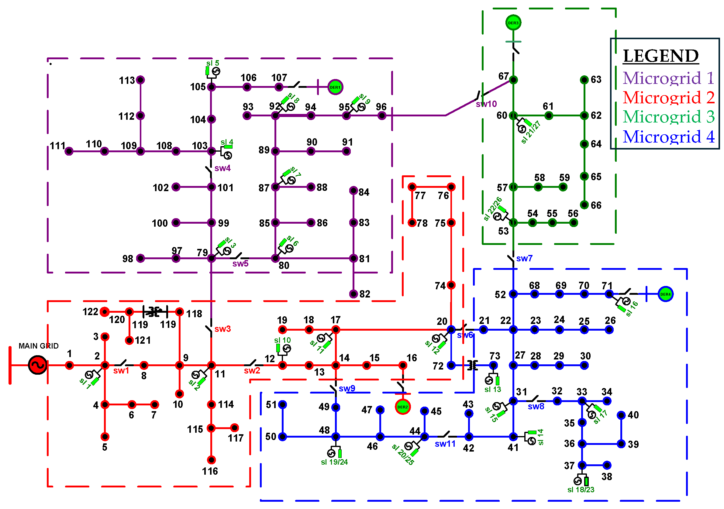
Microgrid No.	Bus No. (GAMS-IEEE 123)	No. DER Resources	UDC Buses
1-Purple	79–18, 80–135, 87–42, 92–47, 95–50, 103–25, 105–29	7	107–251
2-Red	2–1, 11–13, 12–152, 17–57, 20–60,	5	16–56
3-Green	53–197, 60–105,	2	67–350
4-Blue	48–93, 44–91, 41–87, 31–76, 37–82, 33–78, 73–610, 71–450,	8	71–451
Total: 4-Microgrids	22-Buses	22-DER Resources each 130 kW	4-Inverters

and

Table A2. List of nodes with dynamic loads based on the modified IEEE 123-node configuration.

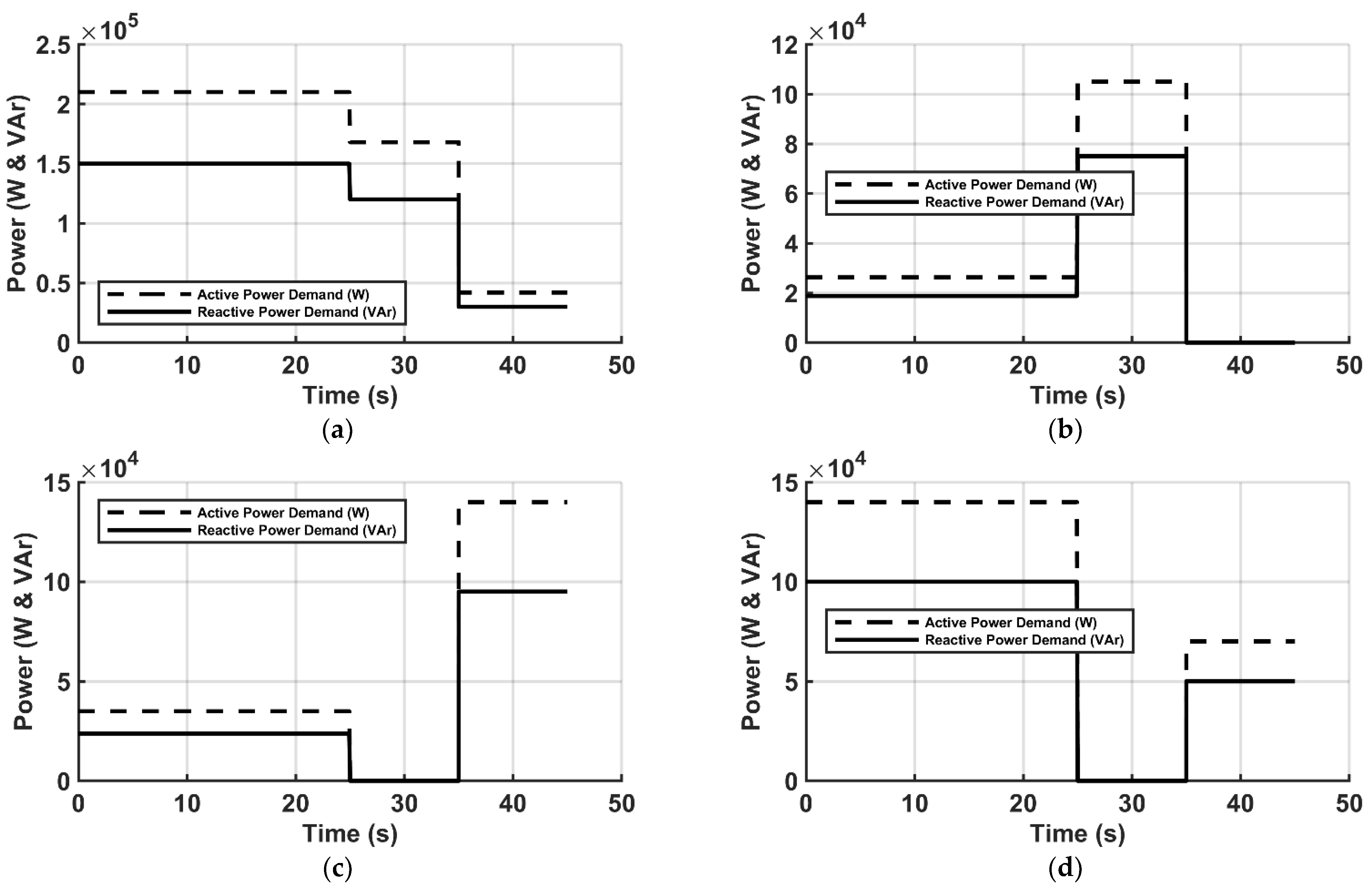
S/N	GAMS-IEEE Nodes	PQ Dynamic Load	Load Curtailment (%)
1	92–47	210 kW & 150 kVAr	100, 80, 20
2	93–48	105 kW & 75 kVAr	20, 100, 0
3	94–49	140 kW & 95 kVAr	20, 0, 100
4	77–65	140 kW & 100 kVAr	100, 0, 50

in Appendix A. Table A2 in the appendix describes the major DERs resources on the network with their GAMS and IEEE standard bus number labels.

The overall system operates without traditional communication protocols; instead, it relies entirely on local measurements and control via droop-based laws. All switching actions and load coordination in the Simulink environment are driven by precomputed GAMS optimization results, which are loaded into the model using “From Workspace” blocks. These blocks provide control signals to dynamic loads, DERs, and decoupled line switches (e.g., lines 13–14 and 14–17), enabling timely responses during microgrid reconfiguration and HILF event simulations. Each GFM inverter functions as a decentralized aggregator using local voltage and frequency measurements, with multiple monitoring points across the network that feed directly into each UDC controller. This decentralized architecture ensures resilience during communication failures, as no real-time data exchange is required between nodes. Even under loss of workspace inputs or partial controller failure, the system remains self-sustaining, unless all inverters become simultaneously inoperative, a highly improbable scenario.

The choice of droop and PI control parameters in this work is guided by a combination of heuristic tuning and established practices from relevant literature while considering the specific dynamic and transient characteristics of the test network. Heuristic methods were used to iteratively adjust parameters based on the system’s voltage and frequency response during simulations. Grid dynamics, such as gradual load changes and renewable intermittency, informed the droop control settings to ensure stable power-sharing and voltage regulation under varying load conditions. For transient events like faults and switching operations, PI controller parameters ($k_{P_i}\mathrm{a}\mathrm{n}\mathrm{d}{k}_{Q_i})$ were tuned to provide fast and stable response, minimizing overshoot and settling time. The effectiveness of these parameters was validated through simulation under various operating scenarios, ensuring the control strategy maintains synchronization and supports both steady-state and dynamic stability.

The main tunable parameters used in the GFM-UDC control include the droop coefficients (Q-V droop gains, and P-f droop gains), voltage controller proportional gain ($k_p$), and voltage controller integral gain ($k_i$), while other parameters like upper and lower limits of each voltage loop output and active/reactive power outputs depend on the output of the tunable parameters. The rated system frequency ($f_o$), system nominal voltage ($V_o$), inverter nominal ratings, filter inductance/capacitance, and network topology constraints are heuristically selected based on documentation, which are fixed parameters. Tuning the Q-V droop gain controls the inverter’s output voltage, the P-f droop gain controls the inverter’s output frequency, necessary for synchronization of parallel inverters and network stability [41,42,43].

In general, the following are considered in selection of appropriate parameter values: (a) system stability must be guaranteed under diverse operating conditions; (b) power sharing capability, which droop coefficients are responsible for in the design; (c) dynamic response-tuning PI controller gains to achieve desired transient response characteristics, such as damping, settling time, and overshoot; (d) operational limits, which set overload and reactive power limit controller gains to prevent inverter operation beyond specified limits; and (e) noise rejection, which is controlled by the choice of appropriate filter time constants (${\tau }_f$) to establish a balance between system noise rejection and responsiveness.

The tuning implementation is carried out in the MATLAB Control Toolbox under the PID tuner. A system with 8-Core Processor, 4501Mhz, RAM-64GB, x64-based PC was used with MATLAB R2023a-Simulink, and GAMS 43.3.1 version for numerical optimization of the network. The various simulated operating conditions on the network are performed during a 45 s simulation time window. All the network parameters can be accessed in Appendix A and the referenced documentation [44].

4.1. Simulation Results and Discussions

Measurement Metrics Used

Network measurement metrics used in this work include percentage voltage deviation, frequency recovery time, optimization run-time, and load curtailment reduction.

Table 1. Network measurements compared with benchmarks.

S/N	Evaluation Metrics	GFM-UDC Approach	Benchmark
1	Voltage deviation (%)	2.8%	±5%
2	Frequency recovery time	1.57s	2–5 s
3	Optimization run-time	54 s	1–5 min
4	Load curtailment reduction	25.24%	Up to 30%
5	Active power loss (%)	0.4%	5% of total load

presents vital network metrics used in this work as the basis for comparing the approach with the benchmark values using other models [44].

Table 1 indicates minimized voltage deviation of 2.8% with frequency recovery time of 1.57 s as compared with the benchmark. The optimization run-time is significantly reduced as compared with the benchmark value for a distribution network. Load curtailment is reduced by up to 25.24% as compared with the base case. A 0.4% network active power loss reduction is also recorded as compared to the benchmark value of 5% of total load. The microgrids’ frequency levels are stabilized with synchronized inverters with reduced frequency recovery time after each simulated HILF event on the network, as shown in Figure 7 and Figure 8.

The frequency spikes in Figure 7a,b show the fault levels, which help in localizing the probable fault location on the network.

The measured frequency from inverter-2 highlights two network events—normal and abnormal operating conditions—with the latter caused by intentional disconnections of lines and loads. Figure 7a depicts two zones (A and B), where zone A represents the grid-tied operation mode of the network, and zone B is the island mode of operation with HILF events simulated. Zone B shows pronounced frequency spikes that indicate abnormal network conditions. At 25 s, a major spike aligns with the disconnection of dynamic loads.

At 30 s, the line disconnection between nodes 14–17 caused further upward frequency spikes, followed by reconnection after 5 s, and additional line adjustments between buses 13 and 14 from 35 s to 40 s. These frequency fluctuations indicate high-impact low-frequency (HILF) events, that correlate with spikes observed at inverters-1, -3, and -4 in Figure 7b and Figure 8a,b, confirming faults near them as they exhibit the most pronounced spikes.

The network phase voltages were equally monitored from the four (4) nodal grid-forming inverters with UDC capabilities. The measured RMS phase voltages are taken from the four nodal GFM-UDC inverters to validate the global control of the inverters on the network, as shown in Figure 9a–d. Figure 9a revealed smooth transitioning from grid-connected to islanded mode of operation at 20 s by inverter-2. There are voltage fluctuations due to load disconnect on the network at 25 s, line disconnection (between buses 14 and 17) occurred at the 30 s, further line disconnection (between buses 13 and 14) at 35 s, leading to observed spike followed by drop in the network RMS phase voltages measured, and line reconnection at 40 s that resulted in a slight spike in voltage, which was promptly controlled by the UDC-inverter.

Figure 9b–d illustrate the RMS phase voltages measured at inverters-1, -3, and -4, respectively. Figure 9b illustrates pronounced spikes in phase voltages at 35 s and 40 s because inverter-1 is very close to the location of line disconnections (simulated HILF events) and reconnections, respectively. The UDC inverters quickly restored the network phase voltages back to nominal values after the HILF events, thus making the distribution network more resilient to HILF events. The voltage waveforms shown in Figure 9a–d indicate a smooth transition from grid-connected to island modes of operation at 20 s. An insignificant voltage swell due to load curtailment at 25 s. At 30 & 35 s, a major voltage drops occur due to line disconnections and load curtailments.

A line reconnection and simultaneous disconnection occurred at 40 s. It followed the waveform pattern in Figure 9d, confirming the global visibility of the network state from the GAMS optimized UDC-inverters. Figure 9a–d confirm the global visibility of the network and network improved resiliency with UDC-inverter implementation along with GAMS numerical optimization of active network operation, which includes switching operations, load curtailments, and HILF event simulations.

Figure 10a shows a Y-connected PQ load at node 93 with a peak demand of 210 kW real power and 150 kVAr reactive power. The demand response follows a load curve with managed curtailments. Initially, 100% of the load is supported for 25 s. Then, over the next 10 s, noncritical loads are shed, reducing load support to 80%. Between 35 and 45 s, further shedding reduces the load to 20%, following the customer’s load profile. Load control is optimized in GAMS, dynamically adjusting weights for resources across various microgrids with different load schedules. The results of other dynamic loads on the distribution network are shown in Figure 10b–d.

Figure 10b is a Y-connected PQ load-shedding profile on bus 92; dynamic load 2: 92 Y-PQ: P = 105 kW, Q = 75 kVAr. The initial load pick-up follows at 20%, 100%, and 0%. Figure 10c indicates dynamic load 3 on bus 94; 94 Y-PQ: P = 140 kW, Q = 95 kVAr. The initial load pick-up follows at 20%, 0%, and 100%. Figure 10d shows dynamic load 4 at bus 77; 77 D-PQ: P = 140 kW, Q = 100 kVAr. The initial load pick-up follows at 100%, 0%, and 50%. The four dynamic load pick-up percentages are optimized with the GAMS numerical optimization tool. The weights are dynamically allocated to the loads for implementation in the Simulink model of the distribution network, as shown in Figure 6.

The RMS active power at the inverters is presented in Figure 11a,b.

In Figure 11a, the RMS active power at the inverter-4 output was monitored, where the network operates in grid-connected mode in the first 20 s. At 12 s, the GFM-UDC is activated to supply 0.3 p.u. of network total active power from the DERs still in grid-connected mode of operation, and in the 20 s, the microgrid switched to island mode. The grid-forming inverter increased power to support loads, while dynamic loads were shed at 25 s. Lines 14–17 were disconnected at 30 s and reconnected after 5 s, with lines 53–54 disconnected at 35 s and reconnected at 40 s. This demonstrates robust active power flow control and stability, with effective power sharing across IBR resources in grid-tie and island modes of operation. Figure 11b shows the RMS reactive power at DER-4 with significant downward spikes after 30 s, similar to DER-3, which is located near the simulated fault. This indicates that the fault is closer to DER-3 and DER-4 when compared to the other DERs, thus allowing easy localization of the fault. The GFM-UDC design improves fault detection and isolation, as shown by spikes at 35 s, reflecting line restoration and subsequent disconnection.

The rest of the IBR resources network active and reactive power measurements are shown in Figure 12a–f. The observed patterns indicate global visibility of the network from each of the GFM inverters.

This control approach enhances system resilience and stability, maintaining voltage and frequency during abnormal conditions.

4.2. Discussion

4.2.1. Improved System Stability

Figure 13a–d illustrate the effect of proper tuning of the droop and PI controller gains on the system power stability at inverter-4.

The results in Figure 13 illustrate the effects of appropriate parameter settings on the active/reactive power in a power system before and after the tuning at inverter-4. Shown in Figure 13a,b, the system experiences a huge oscillation between 0 and 10 s (about 4 and 8 p.u. in magnitude in active and reactive power) in grid-connected mode, and between 20 and 30 s (island-operation mode), another huge spike occurs in active and reactive power above the recommended level (1 p.u.). Lines 14–17, 13–14 are scheduled for disconnections between (30–35 s) and (35–40 s), respectively. Between 30 and 40 s, HILF events are applied to the networks with line disconnection at 30 s, line reconnection and simultaneous line disconnection carried out at 35 s; thus, there is an upward spike for line reconnection and downward spike for the line disconnections. The untuned UDC network experienced a huge power surge in the range of 8 p.u. deviation from the nominal, while the tuned network achieved a recovery time of 1.57 s and power flow within 1.0 p.u. Although spikes were experienced in both networks, indicating the inception of the HILF events, the fine-tuned network shows that the power stays within the acceptable range of 0–1 p.u. for active power and −1.0 to 1.0 p.u. for reactive power. A careful tuning of P–f droop gain from 0.01 p.u. to 0.015 p.u. achieved better system response while the Q–V gain remains the same (0.01 p.u.) to achieve stable operating conditions under abnormal operating conditions. The initial network instability was eliminated with appropriate parameter settings.

The per-phase voltage after optimizing the network operation is shown in Figure 14.

As shown in Figure 14, the optimized unbalanced 3-ϕ phase bus voltages are maintained within the required voltage range of 0.95 and 1.05 p.u. with percentage voltage deviation of 2.8%, validating the effectiveness of the developed framework. Furthermore, in the grid-tied mode of operation, the active and reactive power output of the GFM inverters is at zero (0) until otherwise set to inject 0.3 p.u. of the total active power requirement of the network via IBR resources. This confirms the robust control capability of the designed GMF-UDC inverter to handle both modes of operation. The GFM-UDC controllers effectively handle the distribution power network transitioning from grid-tied to islanded mode of operation, and dynamic microgrid formation in islanded mode of operation, as shown in Figure 8 (network frequency profile), Figure 9 (network RMS phase voltages), 21–28 (network active and reactive powers). Furthermore, in the face of HILF events discussed earlier, the proposed control mechanism managed the necessary network vitals (frequency and bus voltages) within an acceptable range and experienced improved network recovery time after HILF events. Network resiliency was enhanced with the proposed integrated solution.

Compared with relevant existing models, the results obtained revealed an unparallel benefit in the proposed approach over conventional techniques. In [41], a global solution at times is not guaranteed, especially when the load-end appliance controller loses communication with the inverters in HILF events. In contrast, GAMS-optimized GFM-UDC ensures a global solution even during an HILF event, as the GAMS GFM-UDC system operates independent of traditional communication protocols; instead, it relies entirely on local measurements and control via droop-based laws. In [42], a simulation time of 1407.14 s was recorded with a voltage deviation 0.04 p.u. on the IEEE 123-node distribution network; in contrast, the developed GFM-UDC achieved a simulation time of 107.53 s and 0.028 p.u. voltage deviation. It required about 5 s to recover from the HILF event described in [42]; however, with the GAMS-optimized GFM-UDC, an average of 1.57 s recovery time could be observed from different HILF event scenarios. Also, while a 23.5% reduction in active power loss and 6 s recovery time from secondary frequency transient conditions after optimization was recorded in [43], the GFM-UDC achieved 25.24% reduction in active power loss plus a better secondary frequency recovery time of 1.57 s.

4.2.2. Fault Localization with HHO

The HHO algorithm is implemented for fault detection on the modified IEEE 123-bus distribution network using the bus voltage signatures obtained after simulation along with the extracted bus coordinates. Although the results indicate fast simulation time (0.086 s), the optimal solution accuracy is about 40% on 500 maximum iterations. The low accuracy level could indicate the inability of the HHO algorithm to find a global solution in many instances. Fitness function typically combines classification loss (accuracy), feature dimensionality, and generalization error. The multi-objective HHO convergence curve plot (shown in Appendix A, Figure A1b) reveals the extent to which the solution is accurate. The simulation was run recursively, identifying faulty buses at the ratio of 2:5. However, the GAMS-UDC solution provided a useful analytical solution for fault localization with the fault voltage and frequency signatures, which correspond to the nodes where the HILF events occurred. This is a unique solution that is problem dependent and useful in localizing the faults on the network and making informed decisions by the network operators. The plot of the common points of frequency and voltage spikes coincides with or is close to the bus where the HILF events are applied. Figure A1b presents the output from the HHO algorithm result. Figure A1a,b in Appendix A present the result from the HHO technique for network fault localization using the bus voltage signature of the network simulation output, where the HHO technique could favorably predict the faulty buses.

4.2.3. Applicability for Real-Time Solution and Challenges

The proposed GAMS-MATLAB framework shows potential for real-time applicability under specific conditions. On the modified IEEE 123-bus network, the total simulation time was 107.53 s, with the GAMS-based optimization (using the CPLEX −MIP, SCIP −MINLP solvers) converging in approximately 53 s under 69 constraints. While this timing does not meet strict real-time requirements (typically <1 s for fast control loops), performance can be significantly improved by using linearized models and deploying the framework on high-performance platforms such as OPAL-RT for hardware-in-the-loop (HIL) testing. Among the solvers tested (CPLEX, SOPLEX, IPOPT, SCIP, GUROBI, CBC), CPLEX, SCIP offered the best trade-off between computation time and solution accuracy. Although the MINLP formulation has higher computational complexity (nonpolynomial time in worst cases), the problem size remains tractable for near-real-time applications in slower control layers such as reconfiguration and optimization-based dispatch. The GAMS engine offers scalable and efficient optimization routines that outperform conventional MATLAB solvers in both latency and robustness.

Assuming no communication breakdown between the UDC inverters and the GAMS optimization can be a challenge in a truly complex distribution network with multiple network facilities, as smart and more expensive computational resources will be required to cope with this assumption in a larger distribution network. Another assumption is that of simplified fixed loads and DER models across the network, for the majority of which in real-life may not be the case, leaving this approach to only larger grids with significant computational resources. Managing and processing vast amounts of data from numerous DERs and sensors becomes challenging, and as such, potential delays in decision-making and control actions may arise, compromising the system performance if not carefully managed with GAMS optimization using parallel computing. Ensuring coordinated control among numerous UDC inverters to prevent conflicts and ensure system stability can result in increased complexity in control algorithms and potential for control conflicts when not managed properly. Integrating the GMF-UDC approach with legacy power infrastructure may not support the control strategy or the required advanced communication protocols required by GFM-UDC on a large scale, which may necessitate significant upgrades and increasing implementation costs and communication architecture complexity.

5. Conclusions

This research introduces a multi-layer distribution network optimization approach, integrating GFM-UDC, GAMS, and MATLAB-Simulink to enhance network stability and resilience under abnormal operating conditions. The results demonstrate efficient voltage and frequency stability in response to simulated HILF events in MATLAB-Simulink. By using GAMS to optimize microgrid formation, switching actions, and dynamic load management, the approach effectively stabilizes the system while leveraging available network resources. Additionally, optimal power flow (OPF) solutions in GAMS achieved cost-effective operation by minimizing load loss during HILF events, ensuring a more stable and reliable distribution network. Future work will focus on implementing the developed MATLAB-Simulink model on an OPAL-RT laboratory platform to enable real-time hardware-in-the-loop (HIL) testing. This will provide a realistic and practical testbed for simulating various high-impact low-frequency (HILF) events. The integration with OPAL-RT will allow validation of the control strategies under real-time conditions, bridging the gap between simulation and physical implementation.

References

- An, R.; Liu, Z.; Liu, J.; Liu, B.A. Comprehensive Solution to Decentralized Coordinative Control of Distributed Generations in Islanded Microgrid Based on Dual-Frequency-Droop. IEEE Trans. Power Electron. 2022, 37, 3583–3597. [Google Scholar] [CrossRef]
- Zhang, Z.; Dou, C.; Yue, D.; Zhang, B. Predictive Voltage Hierarchical Controller Design for Islanded Microgrids Under Limited Communication. IEEE Trans. Circuits Syst. 2022, 69, 933–942. [Google Scholar] [CrossRef]
- Xie, X.; Quan, X.; Wu, Z.; Cao, X.; Dou, X.; Hu, Q. Adaptive Master-Slave Control Strategy for Medium Voltage DC Distribution Systems Based on a Novel Nonlinear Droop Controller. IEEE Trans. Smart Grid. 2021, 12, 4765–4772. [Google Scholar] [CrossRef]
- Lin, F.-J.; Tan, K.-H.; Chang, C.-F.; Li, M.-Y.; Tseng, T.-Y. An Improved Droop-Controlled Microgrid Using Intelligent Variable Droop Coefficient Estimation. IEEE J. Emerg. Sel. Top. Power Electron. 2024, 12, 4128–4140. [Google Scholar] [CrossRef]
- Munir, M.S.; Li, Y.W.; Tian, H. Residential distribution system harmonic compensation using priority driven droop controller. IEEE Trans. Power Electron. 2020, 35, 213–223. [Google Scholar] [CrossRef]
- Tu, H.; Yu, H.; Lukic, S. Dynamic Nonlinear Droop Control (DNDC): A Novel Primary Control Method for DC Microgrids. IEEE Trans. Power Electron. 2024, 39, 10934–10944. [Google Scholar] [CrossRef]
- Almeida, A.O.; Almeida, P.M.; Barbosa, P.G. Design Methodology for the DC Link Current Controller of a Series-Connected Offshore Wind Farm with a Droop Control Strategy. IEEE Trans. Ind. Appl. 2024, 60, 3568–3577. [Google Scholar] [CrossRef]
- Gu, M.; Meegahapola, L.; Wong, K.L. Coordinated Voltage and Frequency Control in Hybrid AC/MT-HVDC Power Grids for Stability Improvement. IEEE Trans. Power Syst. 2021, 36, 635–644. [Google Scholar] [CrossRef]
- Prakash, S.; Nougain, V.; Mishra, S. Adaptive Droop-Based Control for Active Power Sharing in Autonomous Microgrid for Improved Transient Performance. IEEE J. Emerg. Sel. Top. Power Electron. 2021, 9, 3010–3020. [Google Scholar] [CrossRef]
- Zhong, Q.C.; Nguyen, P.L.; Ma, Z.; Sheng, W. Self-synchronized synchronverters: Inverters without a dedicated synchronization unit. IEEE Trans. Power Electron. 2021, 29, 617–630. [Google Scholar] [CrossRef]
- Minetti, M.; Rosini, A.; Denegri, G.B.; Bonfiglio, A.; Procopio, R. An Advanced Droop Control Strategy for Reactive Power Assessment in Islanded Microgrids. IEEE Trans. Power Syst. 2022, 37, 3014–3023. [Google Scholar] [CrossRef]
- Tavakoli, S.D.; Sánchez-Sánchez, E.; Prieto-Araujo, E.; Gomis-Bellmunt, O. DC Voltage Droop Control Design for MMC-Based Multiterminal HVDC Grids. IEEE Trans. Power Deliv. 2020, 35, 2414–2424. [Google Scholar] [CrossRef]
- Ambia, M.N.; Meng, K.; Xiao, W.; Al-Durra, A.; Dong, Z.Y. Adaptive Droop Control of Multi-Terminal HVDC Network for Frequency Regulation and Power Sharing. IEEE Trans. Power Syst. 2021, 36, 566–577. [Google Scholar] [CrossRef]
- Ghanbari, N.; Bhattacharya, S. Adaptive Droop Control Method for Suppressing Circulating Currents in DC Microgrids. IEEE Open Access J. Power Energy 2020, 7, 100–110. [Google Scholar] [CrossRef]
- Wang, X.; Zhang, J.; Zheng, M.; Ma, L. A distributed reactive power sharing approach in microgrids with improved droop control. CSEE J. Power Energy Syst. 2021, 7, 1238–1245. [Google Scholar]
- Xu, Y.; Liu, C.-C.; Schneider, K.P.; Ton, D.T. Placement of remote-controlled switches to enhance distribution system restoration capability. IEEE Trans. Power Syst. 2016, 31, 1139–1150. [Google Scholar] [CrossRef]
- Saleh, A.; Rastegarnia, A.; Farzamnia, A.; Kin, K.T.T. Power and Current Limiting Strategy Based on Droop Controller with Floating Characteristic for Grid-Connected Distributed Generations. IEEE Access 2022, 10, 13967–13973. [Google Scholar] [CrossRef]
- Wang, Y.; Wang, Z.; Lei, M.; Qiu, F. Analysis and Control of DC Voltage Dynamics Based on a Practical Reduced-Order Model of Droop-Controlled VSC-MTDC System in DC Voltage Control Timescale. IEEE Trans. Power Deliv. 2024, 39, 1031–1038. [Google Scholar] [CrossRef]
- Dissanayake, A.M.; Ekneligoda, N.C. Multiobjective Optimization of Droop-Controlled Distributed Generators in DC Microgrids. IEEE Trans. Ind. Inform. 2020, 16, 2423–2435. [Google Scholar] [CrossRef]
- Shin, D.-Y.; Kwon, D.-H.; Moon, S.-I.; Yoon, Y.-T. Real-Time Coordinated Control of a Grid-VSC and ESSs in a DC Distribution System for Total Power Loss Reduction Considering Variable Droop Using Voltage Sensitivities. IEEE Access 2023, 11, 8300–8312. [Google Scholar] [CrossRef]
- Majumder, R. Some aspects of stability in microgrids. IEEE Trans. Power Syst. 2013, 28, 3243–3252. [Google Scholar] [CrossRef]
- Zhao, X.; Liu, J.; He, J. Experimental validation of UDC-based inverter control in hardware-in-the-loop microgrid. Electr. Power Syst. Res. 2022, 209, 107950. [Google Scholar]
- Tan, J.; Zhong, H.; Xia, Q. Unified grid-interactive inverter design for resilience-oriented microgrid control. IEEE Access 2022, 10, 35491–35504. [Google Scholar]
- Lasheen, A.; Ammar, M.E.; Zeineldin, H.H.; Shaaban, M.F.; El-Saadany, E. Assessing the Impact of Reactive Power Droop on Inverter Based Microgrid Stability. IEEE Trans. Energy Convers. 2021, 36, 2385–2395. [Google Scholar] [CrossRef]
- Zhang, Y.; Wang, L.; Li, W. Autonomous DC Line Power Flow Regulation Using Adaptive Droop Control in HVDC Grid. IEEE Trans. Power Deliv. 2021, 36, 3550–3561. [Google Scholar] [CrossRef]
- Du, W.; Tuffner, F.K.; Schneider, K.P.; Lasseter, R.H.; Xie, J.; Chen, Z.; Bhattarai, B. Modeling of grid-forming and grid-following inverters for dynamic simulation of large-scale distribution systems. IEEE Trans. Power Del. 2021, 36, 2035–2045. [Google Scholar] [CrossRef]
- Schneider, K.P.; Radhakrishnan, N.; Tang, Y.; Tuffner, F.K.; Liu, C.C.; Xie, J.; Ton, D. Improving primary frequency response to support networked microgrid operations. IEEE Trans. Power Syst. 2019, 34, 659–667. [Google Scholar] [CrossRef]
- Schneider, K.P.; Tuffner, F.K.; Elizondo, M.A.; Liu, C.-C.; Xu, Y.; Ton, D. Evaluating the feasibility to use microgrids as a resiliency resource. IEEE Trans. Smart Grid. 2017, 8, 687–696. [Google Scholar]
- Yao, Y.; Liu, W.; Jain, R. Power System Resilience Evaluation Framework and Metric Review. In Proceedings of the IEEE PES Innovative Smart Grid Technologies Conference, New Orleans, LA, USA, 24–28 April 2022. [Google Scholar]
- He, J.; Li, Y.W. An Enhanced Microgrid Load Demand Sharing Strategy. IEEE Trans. Power Electron. 2012, 27, 3984–3995. [Google Scholar] [CrossRef]
- Olivares, D.E.; Mehrizi-Sani, A.; Etemadi, A.H.; Canizares, C.A.; Iravani, R.; Kazerani, M.; Hajimiragha, A.H.; Gomis-Bellmunt, O.; Saeedifard, M.; Palma-Behnke, R.; et al. Trends in Microgrid Control. IEEE Trans. Smart Grid 2014, 5, 1905–1919. [Google Scholar] [CrossRef]
- Farrokhabadi, M.; Ca, C.A.; Bhattacharya, K. Power Quality in Microgrids: An Overview. IEEE Access 2018, 6, 29587–29612. [Google Scholar]
- Yazdani, A.; Iravani, R. Voltage-Sourced Converters in Power Systems: Modeling, Control, and Applications; IEEE Press: Piscataway, NJ, USA, 2010; pp. 3–12. [Google Scholar]
- Savaghebi, M.; Jalilian, A.; Vasquez, J.C.; Guerrero, J.M. Secondary Control Scheme for Voltage Unbalance Compensation in an Islanded Droop-Controlled Microgrid. IEEE Trans. Smart Grid. 2012, 3, 797–807. [Google Scholar] [CrossRef]
- Xue, N.; Wu, X.; Gumussoy, S.; Muenz, U.; Mesanovic, A.; Dong, Z.; Bharati, G.; Chakraborty, S. Dynamic security optimization for N-1 secure operation of power system with 100% non-synchronous generation: First experiences from Hawaii Island. In Proceedings of the PES General Meeting, Washington, DC, USA, 26–29 July 2021. [Google Scholar]
- Heidari, A.A.; Mirjalili, S.; Faris, H.; Aljarah, I.; Mafarja, M.; Chen, H. Harris hawks optimization: Algorithm and applications. Future Gener. Comput. Syst. 2019, 97, 849–872. [Google Scholar] [CrossRef]
- Tan, Z.; Zhang, Y.; Liu, X.; Wang, H.; Li, J.; Zhang, Y.; Wang, L.; Li, W.; Zhang, Z.; Liu, Y. Entropy-enhanced few-shot learning with HHO for industrial machinery fault classification. Expert Syst. Appl. 2023, 210, 118533. [Google Scholar]
- Zhang, M.; Wang, D.; Xu, Y.; Zhang, H.; Feng, G.; Wang, H.; Gu, F.; Sinha, J.K.; Zhang, H.; Feng, G. Few-shot fault diagnosis using meta-learning and entropy-optimized deep features. IEEE Trans. Ind. Inform. 2022, 18, 133–143. [Google Scholar]
- Liu, Z.; Li, W.; Gao, M.; Zhang, Z.; Wang, R.; Guan, C.; Wang, Q.; Zhang, Z.; Li, W.; Gao, M. Multi-scale CNN with HHO optimization for intelligent fault diagnosis. Measurement 2021, 178, 109401. [Google Scholar]
- Guo, Y.; Zhang, Z.; Li, W.; Wang, R.; Guan, C.; Wang, Q.; Zhang, Z.; Li, W.; Wang, R.; Guan, C. Fault diagnosis based on image entropy fusion and deep CNN. IEEE Access 2021, 9, 45522–45534. [Google Scholar]
- Schneider, K.P.; Tuffner, F.K.; Elizondo, M.A.; Liu, C.-C.; Xu, Y.; Backhaus, S.; Ton, D. Enabling Resiliency Operations Across Multiple Microgrids with Grid Friendly Appliance Controllers. IEEE Trans. Smart Grid 2018, 9, 4755–4764. [Google Scholar] [CrossRef]
- Li, P.; Ji, H.; Wang, C.; Zhao, J.; Song, G.; Ding, F.; Wu, J. Coordinated Control Method of Voltage and Reactive Power for Active Distribution Networks Based on Soft Open Point. IEEE Trans. Sustain. Energy 2017, 8, 1430–1442. [Google Scholar] [CrossRef]
- Zeng, Y.; Wang, Y.; Li, P. Unified Active and Reactive Power Coordinated Optimization for Unbalanced Distribution Networks in Radial and Looped Topology. Front. Energy Res. 2022, 9, 840014. [Google Scholar] [CrossRef]
- Du, W.; Liu, Y.; Tuffner, F.K.; Huang, R.; Huang, Z. Model Specification of Droop-Controlled, Grid-Forming Inverters (GFMDRP_A), Pacific Northwest National Laboratory: Richland, WA, USA. 2021. Available online: https://www.pnnl.gov/main/publications/external/technical_reports/PNNL-32278.pdf (accessed on 30 June 2023).
- IEEE PES Distribution System Analysis Subcommittee. IEEE 123 Node Test Feeder Benchmark Documentation. IEEE Power and Energy Society. 2010. Available online: https://site.ieee.org/pes-testfeeders/resources/ (accessed on 1 April 2023).