Abstract
In this study, we propose an innovative inner–outer loop control framework for a quadcopter unmanned aerial vehicle (UAV) that significantly enhances the trajectory-tracking speed and accuracy while enhancing robustness against external disturbances. The inner loop employs a Linear Active Disturbance Rejection Controller (LADRC) and the outer loop a proportion integral differential (PID) controller, unified within a fuzzy control scheme. We introduce a Self-Adaptive Bald Eagle Search Optimization algorithm to optimize the initial controller settings, thereby accelerating convergence and improving parameter-tuning precision. Simulation results show that our proposed controller outperforms the conventional two-loop cascade PID configuration, as well as alternative strategies combining an outer-loop PID with a second-order inner-loop LADRC or a fuzzy-enhanced PID-LADRC approach. Moreover, the system maintains the desired position and attitude under external perturbations, underscoring its superior disturbance-rejection capability and stability.
1. Introduction
In recent years, quadrotor unmanned aerial vehicles (UAVs) have been widely used in various fields, including the military, agriculture, and logistics, due to their uncomplicated structure, strong maneuverability, and flexible operation [1,2,3,4,5,6]. The control effectiveness of quadcopter UAVs is greatly affected by their characteristics as a highly coupled, nonlinear, and multivariable system. The strong coupling among the channels causes them to interfere with one another, resulting in control instability and overshooting. Additionally, nonlinearity decreases the accuracy of the model, while the multivariate nature of the inputs and outputs creates a high degree of correlation among them, leading to complex interactions. This makes them particularly susceptible to external environmental disturbances and system uncertainties. As a result, enhancing the control accuracy, stability, and resistance to wind disturbances in quadrotor UAVs has become a central focus in UAV research [7,8].
The utilization of conventional control algorithms, such as proportion integral differential (PID) control, has emerged as a pervasive practice in the design of quadrotor UAV control systems. This preference can be attributed to the inherent simplicity and straightforward implementation characteristics of these algorithms [9,10]. Conventional unmanned aerial vehicle (UAV) control methodologies frequently employ inner–outer loop cascade proportional integral derivative (PID) control, wherein the outer loop governs the position through the regulation of speed, while the inner loop manages the attitude by regulating angular velocity. However, due to the limited performance of PID control in handling strong nonlinearities and complex dynamic systems, [11] extended the original PID control by incorporating fuzzy logic and self-tuning fuzzy parameters using the Extended Kalman Filter (EKF) algorithm. An intelligent selection technique and proactive fuzzy parameter adjustment were proposed to reduce computation time. In [12], the PID parameters were optimized through the implementation of a differential evolution algorithm, which helps to reduce the energy consumption during each trajectory movement of the quadrotor UAV. In [13], the Particle Swarm Optimization (PSO) algorithm was applied to tune the PID parameters, and the results showed that the absolute error fitting function provided optimal PID parameters, which resulted in a lower overshoot, better settling time, and higher setpoint performance compared to other methods.
The Active Disturbance Rejection Control (ADRC) concept was first introduced by Professor Han Jingqing, a Chinese scholar, in 1998 [14]. Professor Han initially introduced this control theory and continued to improve on and promote it in subsequent research. ADRC is a control technology that functions without the use of models. It was specifically designed for systems with unknown dynamics and external disturbances. The system′s primary function is to improve its resilience by estimating and compensating for disturbances in real time, eliminating the need for a comprehensive system model. In [15], ADRC was applied to the control system of quadrotor UAVs, and a double-loop ADRC controller was established. The simulation results showed that this control scheme could maintain stability and accurately track the target even under external disturbances. Professor Gao Zhiqiang simplified Professor Han′s ADRC into a linear form, resulting in LADRC [16]. LADRC connects ADRC parameters to controller and observer frequencies, transforming parameter tuning into a simpler bandwidth adjustment problem, thereby streamlining controller design and implementation. In [17,18], the LADRC controller was implemented in the control system of the quadrotor UAV, and the estimation of total disturbance is achieved through the utilization of a linear extended state observer, while a linear feedback control module is employed to compensate for the disturbance. The designed LADRC system effectively estimated and mitigated the overall disturbance′s effect on the UAV′s attitude. In [19], fuzzy control was incorporated into the LADRC controller to attain peak performance levels through continuous real-time optimization of the controller parameters of the LADRC system. The outcomes demonstrated that the suggested control technique considerably enhanced the responsiveness and the capacity to reject disturbances, and the UAV’s tracking control signal and disturbance compensation ability were significantly enhanced. In [20], the PSO method was utilized to tune the parameters of the LADRC controller, solving the difficulty of tuning too many parameters. The results indicated that the optimized LADRC controller significantly improved the tracking speed.
Sliding mode control (SMC) is a widely used nonlinear control method in various engineering fields. The fundamental concept underpinning this system is the design of a sliding surface, along which the system′s state is intended to move to achieve the desired level of control. SMC has the advantages of strong robustness and fast response; the aforementioned property renders the system especially suitable for contexts characterized by significant uncertainty and external disturbances. In [21], SMC was applied to the quadrotor UAV, and the simulation results demonstrated that this control strategy could drive the quadrotor UAV to accurately reach the given position and yaw angle while maintaining stability even under external disturbances. With the continuous development of control systems, more and more improved sliding mode control strategies have been applied to UAVs. The authors of [22] proposed a model-free terminal sliding-mode control (MFTSMC) strategy intended to regulate both the attitude and position of the quadrotor UAV, with the results showing better tracking performance than PID, backstepping, and sliding mode control. In [23], a controller, designed to function in an adaptive sliding mode, was proposed based on a positive correlation. This controller was developed according to a Lyapunov configuration, continuously correcting the feedback signal to achieve dynamic balance. In [24], an adaptive terminal sliding mode control was proposed, combining PID with sliding mode control, where the control strategy proved to be able to track and stabilize the quadrotor UAV′s state within a finite time under both known and unknown upper bounds of external disturbances, using Lyapunov stability theory. In [25], a new control strategy combined adaptive RBFNN with double-loop IntSMC for improved performance. By combining the advantages of IntSMC with the arbitrary function approximation capability of RBFNN, the method achieved convergence to the desired value in a shorter time. The findings indicated the efficacy and resilience of the proposed control law.
Currently, most controllers are complicated due to the substantial number of control parameters present, and the tuning process often relies on manual experience, making parameter optimization difficult. To address this issue, there is an increasing prevalence of intelligent optimization algorithms that are being applied to quadrotor UAV control systems. In [26], a gravitational optimization algorithm is proposed to improve the parameters of the backstepping controller using Integral Absolute Error (IAE) as the fitness function. The findings demonstrated that the enhanced control performance was optimized, and good tracking effects were achieved. In [27], the implementation of an enhanced whale optimization algorithm was undertaken to address the slow convergence rate and low accuracy of traditional whale optimization algorithms. Using the improved algorithm to adjust the error correction coefficient of the ADRC controller, the results indicated that the control strategy improved system responsiveness and decreased steady-state error. In [28], the pigeon-inspired optimization (PIO) algorithm is proposed to optimize the parameters of the Linear Quadratic Regulator (LQR) controller. This algorithm simulates the behavior of pigeons during migration using geomagnetic fields and visual navigation. The algorithm exhibits advantageous properties, including rapid convergence and a robust global search capability. The findings demonstrated that, in comparison to the PSO algorithm, the PIO algorithm was capable of identifying optimized parameters more efficiently. In [29], the genetic algorithm (GA) was employed to optimize the PID controller parameters. It leverages genetic operators—selection, crossover, and mutation—to emulate natural evolution and iteratively converge on an optimal solution. Simulation results demonstrated that the GA-optimized PID controller substantially enhanced overall system performance, enabling fast and stable tracking of the given trajectory. In [30], the Kriging surrogate optimization algorithm was used to adjust the parameters of the ADRC controller. This algorithm is a methodological framework based on the principles of the Kriging model widely used in the parameter optimization and prediction of complex systems. By using known sample responses to predict the response at unknown points and estimate prediction errors, this algorithm has high accuracy and reliability. Experimental results showed that after optimization, the ADRC controller′s response speed improved and steady-state error decreased, demonstrating the effectiveness of this optimization algorithm.
This paper presents an innovative nested inner–outer loop control model designed to significantly enhance parameter tuning efficiency while effectively mitigating the influence of complex external disturbances on UAVs. The model is based on the dynamics of a quadrotor UAV system. In the position control, we use a state-of-the-art fuzzy PID controller that is optimized through the advanced SABES method. In attitude control, we implement a fuzzy control second-order LADRC, also refined using the SABES algorithm. This advanced SABES algorithm not only improves optimization capabilities but also accelerates convergence, ensuring superior performance. A key highlight of our approach is the fuzzy control mechanism, which enables real-time adjustments to the parameters of both the PID and LADRC controllers, allowing for dynamic responses to varying disturbances and effectively minimizing their impact. To evaluate the effectiveness of this control strategy, we conducted a series of comparative simulations. These simulations aimed to compare our approach with the conventional two-loop cascade PID control, as well as hybrid configurations that combine outer-loop PID with inner-loop LADRC. Additionally, we assessed the PID-LADRC control strategy under fuzzy control modulation. The results of these rigorous simulations robustly validate our approach, demonstrating its remarkable ability to accurately track reference trajectories while adeptly suppressing external disturbances.
2. Quadrotor Modeling
A conventional quadrotor UAV consists of three primary components: the fuselage, the electronics, and the rotors. The fuselage comprises two intersecting rods with rotors symmetrically mounted at their extremities. The configuration under scrutiny here can be shown to guarantee that propellers situated near one another rotate in directions that are opposed. This ensures the maintenance of zero net torque around the central axis and serves to avert the occurrence of uncontrolled spinning. This paper presents the construction of an X-type quadrotor UAV, as depicted in Figure 1, which illustrates its three rotational and three translational axes. The rotational motion about the lateral and longitudinal axes corresponds to roll and pitch, respectively, while yaw represents rotation about the vertical axis. In rotor-based UAVs, the pitch angle controls motion along the vertical axis, whereas the roll angle governs movement along the horizontal axis.
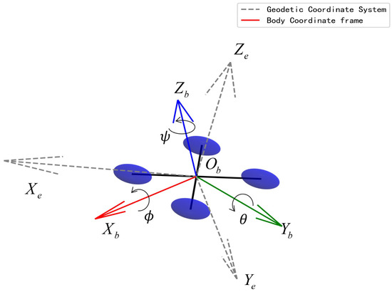
Figure 1.
Schematic diagrams of different coordinate systems.
Determining the altitude and orientation of a UAV with six degrees of freedom necessitates the implementation of two coordinate systems: geodetic and airframe coordinate systems. These systems are employed to ascertain the position and attitude of the UAV in flight, utilizing the transformation matrix , as delineated in Equation (1):
Employing Newton′s and Euler′s laws of motion, we can derive the kinematic equations for the quadrotor UAV in consideration:
In the equations, are moments of inertia around the ; is the total thrust; represent the control input; is wheelbase; represent the drag coefficients for translation and rotation around the three axes, respectively.
The relation between Euler angle and the body angular speed can be described as follows:
When the roll and pitch angles are very small, Equation (3) can be simplified as .
The control inputs , for the quadrotor UAV correlate with the rotational speeds of the four rotor motors as follows:
In the equation, is the thrust coefficient, and is the counter-torque coefficient.
In this study, to focus on the verification of the proposed control algorithm and reduce model complexity, we made the following idealized assumptions in the quadrotor UAV dynamics: air resistance and wind disturbances are neglected, the UAV structure is assumed to be perfectly rigid with no elastic deformation, the thrust and torque generated by the propellers are considered to be linearly controllable, and actuator delays or saturations are ignored. These assumptions are generally valid under controlled indoor environments with little or no wind and for small-scale quadrotor platforms operating at low to moderate speeds. Under such conditions, the influence of aerodynamic drag and external disturbances is limited, and the simplified model provides sufficient accuracy for early-stage controller development and simulation-based performance evaluation. If these assumptions do not hold in real-world applications, the following effects may arise: degraded control performance, such as steady-state error or increased response delay; reduced robustness, potentially leading to instability or large overshoot and discrepancies between simulation and experimental results due to unmodeled dynamics.
3. Controller Design
To tackle the challenges associated with the highly coupled nature, nonlinearity, and under-driving of quadrotor UAV systems, we propose a novel control structure that incorporates both inner and outer loops. The outer loop employs a fuzzy PID controller, while the inner loop consists of a fuzzy control second-order LADRC. The initial parameters for both controllers are optimized using a SABES algorithm. The overall system architecture is depicted in Figure 2.
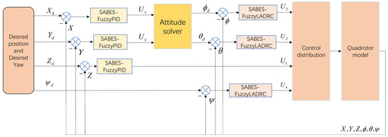
Figure 2.
Control system general block diagram.
3.1. Self-Adaptive Bald Eagle Search Algorithm
The Bald Eagle Search Algorithm (BES), introduced by Alsattar et al. in 2020 [31], was inspired by the hunting process of bald eagles. This algorithm mimics three key stages of the condor′s foraging process: exploration, exploitation, and attack. The algorithm is simple to implement and suitable for global exploration and local development. However, because the algorithm has problems such as high-dimensional complex problems easily falling into local optimization, slow convergence speed, and difficulty determining the parameters, Sharm et al. [32] introduced Dynamic Opposites Learning (DOL) to form the SABES through the setting of the time-varying parameter adaptation.
In the traditional BES:
In the search stage, bald eagles fly randomly through the search space to find prey, and the initial BES uses a flight strategy:
where is a random variable with values in the range of [0, 1], is an algorithm parameter with values in the range of [1.5, 2], represents the best position searched for, and represents the average of the positions searched for.
In the predation stage, the bald eagle selects the best individual (the current optimal solution) to move towards:
where
The algorithm parameter is in the range of [5, 10], the random variable is in the range of [0, 1], and the search period is in the range of [0.5, 2].
The attack phase, in which the algorithm performs a fine-grained search in the vicinity of the current local optimum, is as follows:
where
The algorithm’s parameters take values in the range of [1, 2], and the algorithm’s parameter takes values in the range of [5, 10].
The deployment of the vulture optimization algorithm can be achieved by the above steps, but due to the disadvantages of uncertainty in the parameters of the algorithm and the tendency to fall into local optima, Sharm et al. introduced time-varying parameter adaptation and DOL.
By establishing the mechanism of parameter change over time, linear [33] and nonlinear methods [34] are introduced to select the algorithm’s parameters with the following equations:
where is the exponential adjustment value in the range of [0.9, 1.3], denotes the maximum number of iterations, is the current number of iterations, and denotes the maximum and minimum values of the algorithm’s parameters.
The algorithm employs a nonlinear parameter selection method during the search and hunt phases to enhance its overall search capabilities. In contrast, a linear parameter selection method is used in the attack phase to optimize short boards that are likely to fall into local optima.
The optimal solution and convergence speed of the algorithm are affected by the initial position, so Xu et al. [35] proposed a dynamic opposition learning strategy to avoid entrapment in local optima and accelerate convergence to the global optimum. The DOL equation is as follows:
where denote the lower and upper bounds, denotes the dimension, is a random variable in the range of [0, 1], is obtained according to the pairwise learning method, and denotes the weighting factor.
The operation of the SABES is as follows:
- Use Equation (15) to search for the initialized and dynamic opposing positions, calculate the fitness values for both positions, and select the best search agent based on the best fitness.
- Use Equation (14) to compute the corresponding parameter, after which Equation (5) identifies the current best position and updates the iteration’s position. The fitness value for this iteration is then calculated, and the iteration counter is incremented.
- Calculate the control parameter values using Equation (14) and update the number of iterations by updating the position and the dynamic opposite position using Equations (6)–(9), calculating their fitness values.
- Calculate the values of the algorithm’s parameters using Equation (14), update the current position using Equations (10)–(13), calculate the fitness value for the current iteration, and update the iteration count accordingly.
- Continue to repeat steps 1–4 until the fitness value converges or the number of iterations is reached to stop and obtain the best solution.
To test the merits of the sought value to introduce the fitness function, that is, the time-weighted absolute error integral (ITAE), the size of which can simultaneously reflect the controller on the system′s regulatory speed, overshooting, error, and other aspects of the information, the following formula is defined:
Here, represents current time, and represents the error between the expected value and the true value.
The above steps are used to search for the initial parameters of the LADRC and PID controllers, which are then imported into the corresponding controller modules. For example, the x-position channel is compared with the BES, the PSO algorithm, and the GAPSO algorithm. The iterative changes in the fitness function for different optimization algorithms are shown in Figure 3.
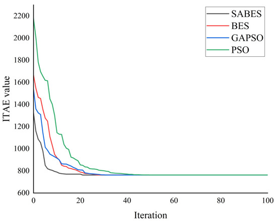
Figure 3.
Convergence curves of fitness functions of different optimization algorithms.
Comparing the fitness function curves of SABES, BES, PSO, and GAPSO over the number of iterations reveals that SABES converges more quickly.
3.2. Fuzzy Control Design
Fuzzy control is a method based on fuzzy logic that addresses uncertainty and complexity. It is particularly suitable for systems where the model is unclear or difficult to describe precisely. The theoretical foundation of fuzzy control was established by Lotfi Zadeh, a renowned American computer scientist, in 1965. The fundamental idea of fuzzy control is to utilize fuzzy sets and fuzzy inference methods to replicate human decision-making processes. Traditional control theory relies on precise numerical values for inputs and outputs, while fuzzy control utilizes fuzzy sets to model uncertainty. A key feature of fuzzy sets is their ability to allow elements to have partial membership, rather than being strictly inside or outside a set. The process of fuzzification, fuzzy inference, and defuzzification—through which outputs are sent to various modules to adaptively adjust the system’s control parameters—is central to the operation of fuzzy control. The fuzzy process is shown in Figure 4.
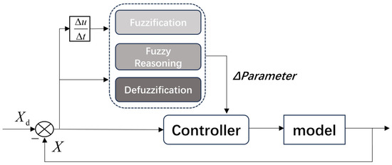
Figure 4.
Fuzzy process.
In the equation, the initialization parameters are obtained by SABES optimization; are the output.
In this study, we used “trimf” for the input and output belonging functions. The fuzzy rule table for is presented in Table 1.

Table 1.
Fuzzy rule for .
Membership functions of the inputs , shown in Figure 5. The outputs are represented by surface plots and membership functions, depicted in Figure 6, Figure 7 and Figure 8.
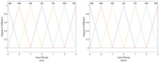
Figure 5.
membership functions.
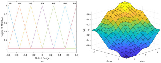
Figure 6.
surface plots and membership function.
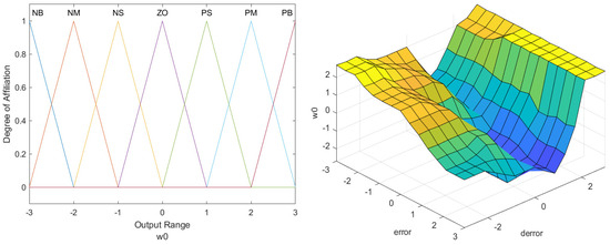
Figure 7.
surface plots and membership function.
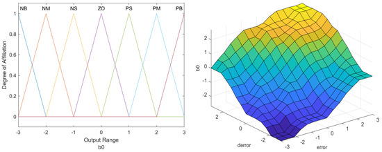
Figure 8.
surface plots and membership function.
Traditional PID controllers are typically tuned empirically, and their performance may not always be optimal. Therefore, to optimize the initial PID parameters, this paper proposes using the SABES algorithm. The following table and figure show the underlying principle and parameter settings.
After optimizing the initial PID parameters using the SABES algorithm, a fuzzy controller is added to enable real-time dynamic adjustment of the PID parameters, thus improving the system′s anti-interference capability. The “trimf” membership function is selected for input and “gaussmf” for output, and the fuzzy rule table is shown in Table 2.
Table 2.
Fuzzy rules for .
Membership functions of the inputs , shown in Figure 9. The output variables are represented by surface plots and membership functions, depicted in Figure 10, Figure 11 and Figure 12.
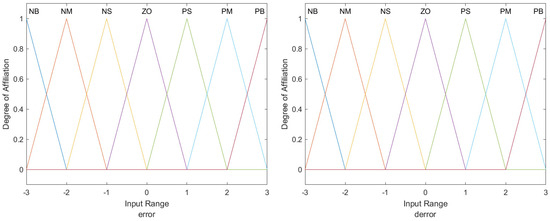
Figure 9.
, membership functions.
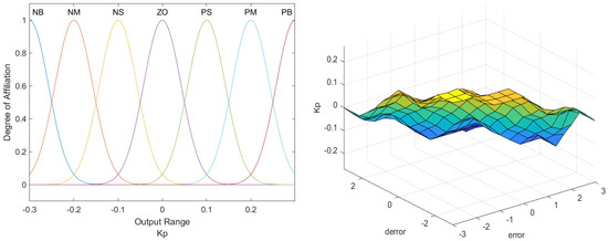
Figure 10.
surface plots and membership function.
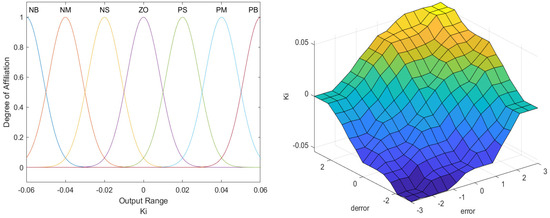
Figure 11.
surface plots and membership function.
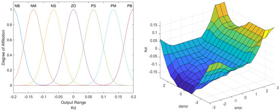
Figure 12.
surface plots and membership function.
The configuration of the inner and outer fuzzy control rules, as well as the fuzzy control parameter ranges, is completed by the aforementioned settings.
3.3. Attitude Control
The attitude controller is a fuzzy control second-order LADRC, optimized using the SABES algorithm, as shown in Figure 13. Unlike the conventional LADRC, this controller combines the SABES algorithm with fuzzy control. The SABES algorithm plays a crucial role in optimally selecting the initial parameters for the LADRC. In contrast, the fuzzy control modifies the LADRC parameters in real time to respond effectively to external uncertainties and disturbances. The components of the LADRC controller include a tracking differentiator (TD), a linear extended state observer (LESO), and a Linear State Error Feedback (LSEF) mechanism.
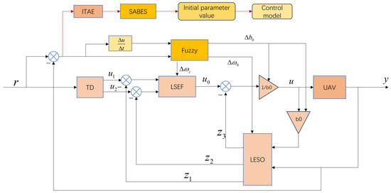
Figure 13.
Structure of attitude controller.
The desired signal is fed into the tracking differentiator to reduce significant initial errors. This process produces two outputs: the first is used for the transition at the tracking point, while the second is used to differentiate the transition at that specific point.
Here, is the target signal; are the analog signal and its derivative. is the factor that adjusts the speed of the tracking signal.
The LESO is tasked with estimating a system′s state variables and disturbances. It achieves this by continuously updating its estimates based on the results from evaluating the system′s output. The dynamic model of the system, which is second-order, can be described as follows:
where represents the total system output, is the control input, is the controller gain, refers to the system state variables, and denotes external disturbances. The total disturbance term is defined by the combination of system state and external disturbances:
Consequently, the dynamic model can be expressed as follows:
The following definition is employed to design the LESO:
The following equation constitutes a formal statement of the state–space equations of the system:
It is hypothesized that the total disturbance varies slowly and is small; therefore, can be approximated as a constant.
To observe , a linear extended observer must be created to estimate it:
Here, is the estimated value of the system state , and is the estimated total disturbance. represent the observer gain and , where is the observer bandwidth and is the compensation factor.
Then, the controller can be described as follows:
Here, represents the complete oversight of the LADRC controller.
The LSEF system integrates the analog signals and their derivatives generated by the TD, with the system states quantities estimated by the LESO through the PD controller. This integration enables the calculation of the virtual control input .
Here, is the analog control input calculated by LSEF. The controller gains are represented by and , while is the controller coefficient.
Frequency Domain Stability Analysis
To verify the controller’s stability, we consider the pitch channel within the attitude control loop as a representative case. In the UAV model, internal coupling effects and external disturbances are collectively defined as the total system perturbation. Accordingly, the pitch-channel dynamics can be expressed as follows:
where represents the total pitch channel perturbation, and denotes the pitch acceleration, which can be derived by applying the Laplace transform to Equations (23)–(26):
where represents the desired value of the pitch angle; it is obtained by substituting Equation (28) into Equation (29):
Assuming that the LESO can accurately observe the amount of perturbation, Equation (27) is derived by applying the Laplace transform to the equation:
This describes the relationship of pitch angle between the actual output and the desired value:
According to Routh′s criterion, a system is considered stable if the conditions and are sufficiently satisfied, thereby confirming the stability of the closed-loop system, as all closed-loop poles reside in the left half of the complex plane. Since represents a controller parameter and is positive, this indicates that the system is indeed stable.
Once the previously mentioned steps are completed, the design of the LADRC controller is considered finalized. However, tuning it can be complicated due to the large number of parameters that must be taken into account, which may prevent optimal performance. Therefore, the next steps will involve using the SABES algorithm to optimize the initial parameters of the LADRC. Following this, a fuzzy control algorithm will be implemented. This series of operations is expected to finalize the design of the attitude control loop.
3.4. Position Control
The block diagram for the position loop control presented in this paper is displayed in Figure 14. The controller utilizes a standard cascaded PID structure, with its initial parameters optimized using the SABES algorithm. The implementation of fuzzy control allows for real-time dynamic adjustments to the controller parameters, improving disturbance rejection performance.
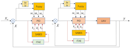
Figure 14.
Structure of position controller.
The PID controller is composed of proportional, integral, and differential control. The proportional term helps to increase the speed of convergence of the feedback value to the target value. The derivative term introduces damping effects to reduce oscillations and overshoots, while the integral term reduces the steady-state error. The addition of fuzzy control results in the identification of three correction functions:
The total expression obtained by combining the three parameters of the PID is given by
Through this process, the SABES algorithm optimizes the controller parameters for both attitude and position loops. Furthermore, a fuzzy control system is configured and integrated to enable real-time dynamic adjustments of the controller parameters.
4. Simulation and Discussion
This paper presents a novel adaptive controller design, a PID-LADRC controller under SABES combined with fuzzy control, which is compared to three conventional controllers: the two-loop cascade PID controller, the outer-loop cascade PID controller combined with the inner-loop LADRC, and the PID-LADRC controller under fuzzy control, referred to as Fuzzy (PID-LADRC). The controllers are designated as SABESFuzzy (PID-LADRC), PID-LADRC, PID-PID, and Fuzzy (PID-LADRC), respectively. All four controllers were implemented using the same quadrotor UAV model. The performance of these controllers, as well as their ability to reject interference, is evaluated by applying identical reference and interference signals.
To validate the proposed controller’s performance in trajectory tracking and disturbance rejection, two simulation scenarios were designed:
- Regular trajectory tracking test: to evaluate the accuracy of tracking under ideal conditions.
- Wind disturbance test: external half-period sinusoidal gusts in three directions are introduced as external perturbations to assess the stability and resilience of the system.
The parameters relevant to the quadrotor UAV are listed in Table 3.
Table 3.
Parameters of quadrotor UAV.
4.1. Simulation of Signal Tracking
The quadrotor UAV’s initial position and orientation were set to (0, 0, 0), corresponding to a zero-velocity condition. The desired flight trajectory is specified in Table 4. The following discussion concentrates on two main aspects: the position tracking results and the tracking error results in Figure 15 and Figure 16.
Table 4.
Desired tracking trajectory.
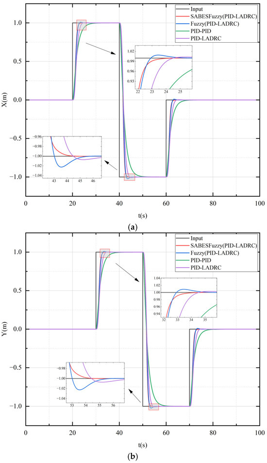
Figure 15.
Tracking results of different channels. (a) X-channel; (b) Y-channel; (c) Z-channel.
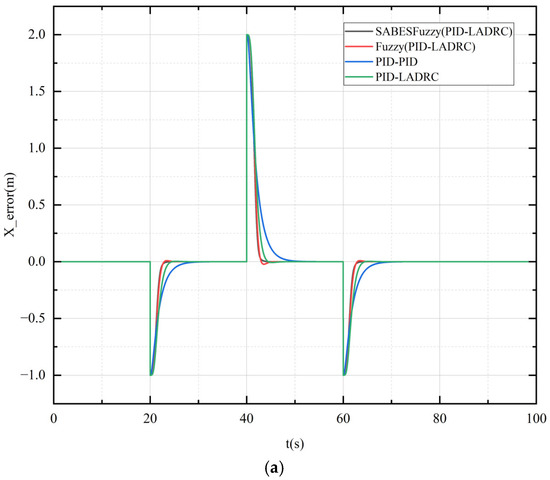
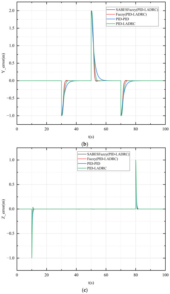
Figure 16.
Tracking error results of different channels. (a) X-channel; (b) Y-channel; (c) Z-channel.
As shown in Figure 15 and Figure 16, in the x-axis direction, the SABESFuzzy (PID-LADRC) controller successfully tracked the desired trajectory from 0 m to 1 m in approximately 4.39 s. In comparison, the Fuzzy (PID-LADRC) controller took 5.09 s to stabilize the tracking of a given signal, and the PID-LADRC and PID-PID controllers required 7.26 s and 12.39 s, respectively, to stabilize and reach the desired trajectory. Notably, the PID-LADRC controller exhibited a slight overshoot of about 0.31%, and the Fuzzy (PID-LADRC) controller exhibited a slight overshoot of about 0.89%, while both the SABESFuzzy (PID-LADRC) and PID-PID controllers achieved the trajectory without any overshoot. Similarly, the SABESFuzzy (PID-LADRC) controller stabilized and tracked the trajectory in approximately 4.17 s over a range of 1 m to −1 m, the Fuzzy (PID-LADRC) controller took 5.41 s, and the PID-LADRC and PID-PID controllers took 7.48 s and 12.67 s, respectively. Additionally, the PID-LADRC controller exhibited a slight overshoot of about 0.73%, and the Fuzzy (PID-LADRC) controller exhibited a slight overshoot of about 2.25%, while both the SABESFuzzy (PID-LADRC) and PID-PID controllers maintained zero overshoot.
As shown in Figure 14 and Figure 15, the SABESFuzzy (PID-LADRC) controller tracked the trajectory from 0 to 1 m in the Z-direction in approximately 1.75 s. In comparison, the Fuzzy (PID-LADRC) took 1.84 s, and the PID-LADRC and PID-PID controllers required 2.3 s and 2.67 s to stabilize and track the desired trajectory. Notably, the PID-LADRC controller exhibited a 3.57% overshoot, while the SABESFuzzy (PID-LADRC), Fuzzy (PID-LADRC), and PID-PID controllers achieved overshoot-free tracking. Furthermore, the SABESFuzzy (PID-LADRC) controller demonstrated excellent performance over the tracking range from 1 m to 0 m, stabilizing in approximately 1.45 s. This represents a significant improvement relative to the Fuzzy (PID-LADRC), PID-LADRC, and PID-PID controllers, which exhibited settling times of 1.50 s, 1.52 s, and 2.08 s, respectively. Moreover, whereas the PID-LADRC configuration experienced a minor overshoot of approximately 0.51%, the SABES-Fuzzy (PID-LADRC), Fuzzy (PID-LADRC), and PID-PID architectures achieved zero overshoot.
The ITAE is adopted as the evaluation criterion for the controllers to facilitate analysis, as illustrated in Table 5. As presented in Table 5, the SABESFuzzy (PID-LADRC) controller exhibits the smallest ITAE value, indicating faster convergence and reduced overshoot compared to the other two controllers. The findings underscore the efficacy of the proposed controller and substantiate the ITAE′s role as an effective evaluation metric.
Table 5.
ITAE values of different channels.
4.2. Simulation of Tracking Signal Response Under External Wind Disturbances
The quadrotor UAV′s initial position and attitude angle were set to (0, 0, 0), and the specified fixed trajectory is shown in Table 6. An external half-period sinusoidal gust was introduced as an external perturbation to the UAV in Table 7. Fixed-point flight simulations were conducted to validate the robustness and efficacy of the proposed control system.
Table 6.
Desired fixed-point hovering trajectory.
Table 7.
External disturbances in different channels.
As shown in Figure 17, the integrated PID and LADRC controllers enhanced by fuzzy control, optimized using the SABES, exhibited faster convergence and stronger resistance to wind disturbances under the same level of gust disturbances compared to the conventional dual-closed-loop PID controllers. The latter were less resistant to external perturbations and exhibited slower recovery in tracking speed. As shown in Figure 18, the fast convergence rate of this new controller resulted in frequent motor adjustments, leading to significant changes in the attitude angle. However, the system quickly reached a steady state.
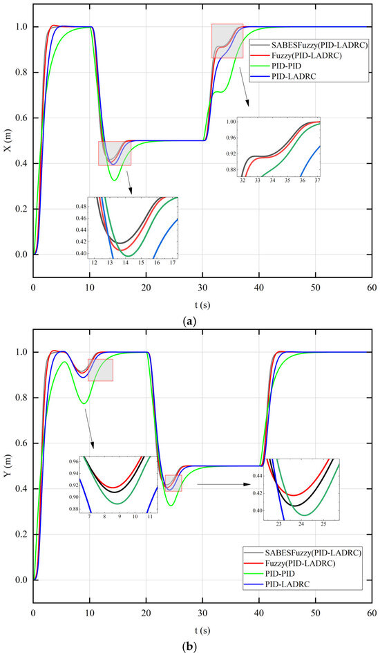
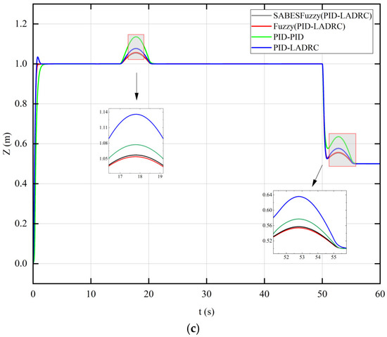
Figure 17.
Tracking results of different channels with wind disturbances. (a) X-channel; (b) Y-channel; (c) Z-channel.
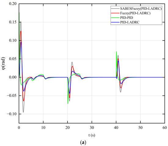
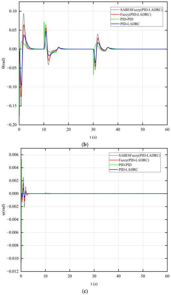
Figure 18.
Attitude tracking results of different channels with wind disturbances. (a) Roll-channel; (b) pitch-channel; (c) yaw-channel.
Take the X-channel as an example: the results show that the SABESFuzzy (PID-LADRC) reduced the maximum overshoot caused by external perturbations by 52.3%, 21%, and 12.7%, and the time to reach the desired trajectory by 28.4%, 6.61%, and 3.78%. In summary, the SABESFuzzy (LADRC-PID) controller presented in this study demonstrates a superior convergence rate, augmented robustness, and enhanced consistency.
5. Conclusions
Given the inherently nonlinear, strongly coupled, and underactuated dynamics of quadrotor UAVs—and their pronounced sensitivity to external disturbances—this paper proposes a novel cascaded inner–outer loop control architecture. The proposed framework significantly enhances robustness against perturbations while substantially improving overall flight performance, improving the effectiveness of small and medium-sized UAVs against small wind disturbances. The primary contributions of this work are summarized as follows:
- The flight dynamics model of the quadrotor UAV was developed based on the Newton–Euler equations, which establish the relationship between position, orientation, and the controller. The control structure consists of two loops: the outer loop uses a fuzzy PID controller optimized by the SABES algorithm, while the inner loop utilizes a fuzzy LADRC, also optimized by the SABES algorithm. The adaptability of the LADRC controller, which does not require an exact model, helps to minimize the impact of nonlinear characteristics on the control strategy. Additionally, the influence of multivariate characteristics is reduced through the use of the SABES optimization algorithm in conjunction with the ITAE optimization objective function, serving as a co-optimization method for the entire system.
- The parameter optimization problem of PID and LADRC controllers is addressed in this paper. An optimization method based on the SABES algorithm is proposed to address the complexity of numerous parameter adjustments in traditional PID and LADRC controllers, as well as the slow convergence issue of the conventional BES algorithm. This adaptive optimization method overcomes the limitation of local optima and enhances the efficiency and accuracy of parameter tuning, thereby resolving the challenges associated with traditional tuning methods.
- The integration of fuzzy control algorithms into the original controller helps mitigate the effects of external disturbances. A set of fuzzy guidelines is established to enable real-time, dynamic modification of the PID and LADRC controller parameters, enabling adaptive changes during disturbances and thereby enhancing the overall stability of the UAV. Most of the existing fuzzy rule designations are based on expert experience, and in the future, data-driven methods (e.g., machine learning, neural networks, etc.) can be added to optimize the outlook of fuzzy rules to improve the controller′s accuracy and adaptive capacity.
- This paper presents a comparative analysis of four types of controllers: PID-PID, PID-LADRC, Fuzzy (PID-LADRC), and SABES-Fuzzy (PID-LADRC). The analysis evaluates their performance under two scenarios: trajectory tracking and external gust interference. The results for both scenarios demonstrate that the proposed control algorithms are highly effective in enhancing resistance to disturbances and improving the speed of tracking.
- Challenges of practical implementation: While the efficacy of the fuzzy controller has been shown through simulations, its implementation in real-world scenarios requires substantial computational resources, placing considerable demands on the computational power, memory, and real-time performance of embedded hardware. Additionally, real-world applications are subject to factors such as sensor noise, model uncertainties, and other variables, which can lead to discrepancies between anticipated and actual performance. Subsequent research endeavors will center on the optimization of the controller to curtail computational demands while preserving accuracy.
Author Contributions
Conceptualization, K.L., Y.B. and G.W.; methodology, K.L. and Y.B.; software, K.L. and Y.B.; validation, K.L. and Y.B.; writing—original draft preparation, K.L.; writing—review and editing, Y.B. and G.W. All authors have read and agreed to the published version of the manuscript.
Funding
Jiangsu Province Natural Science Foundation (BK20130782) of China.
Data Availability Statement
Data are contained within the article.
Conflicts of Interest
The author Guangzhao Wang was employed by the Hangzhou Zhiyuan Research Institute Co. The remaining authors declare that the research was conducted in the absence of any commercial or financial relationships that could be construed as a potential conflict of interest.
References
- Idrissi, M.; Salami, M.; Annaz, F. A Review of Quadrotor Unmanned Aerial Vehicles: Applications, Architectural Design and Control Algorithms. J. Intell. Robot. Syst. 2022, 104, 22. [Google Scholar] [CrossRef]
- Yadav, Y.; Kushwaha, S.K.P.; Mokros, M.; Chudá, J.; Pondelík, M. Integration of Iphone Lidar with Quadcopter and Fixed Wing Uav Photogrammetry for the Forestry Applications. Int. Arch. Photogramm. Remote Sens. Spat. Inf. Sci. 2023, XLVIII-1/W3-2023, 213–218. [Google Scholar] [CrossRef]
- Nath Tripathi, R.; Ghazanfarullah Ghazi, M.; Badola, R.; Ainul Hussain, S. Feasibility Study of UAV Based Ecological Monitoring and Habitat Assessment of Cervids in the Floating Meadows of Keibul Lamjao National Park in Manipur, India. Measurement 2024, 229, 114411. [Google Scholar] [CrossRef]
- Tang, P.; Li, J.; Sun, H. A Review of Electric UAV Visual Detection and Navigation Technologies for Emergency Rescue Missions. Sustainability 2024, 16, 2105. [Google Scholar] [CrossRef]
- Wang, L.; Xia, S.; Zhang, H.; Li, Y.; Huang, Z.; Qiao, B.; Zhong, L.; Cao, M.; He, X.; Wang, C.; et al. Tank-mix Adjuvants Improved Spray Performance and Biological Efficacy in Rice Insecticide Application with Unmanned Aerial Vehicle Sprayer. Pest Manag. Sci. 2024, 80, 4371–4385. [Google Scholar] [CrossRef]
- Wongsuk, S.; Qi, P.; Wang, C.; Zeng, A.; Sun, F.; Yu, F.; Zhao, X.; Xiongkui, H. Spray Performance and Control Efficacy against Pests in Paddy Rice by UAV-based Pesticide Application: Effects of Atomization, UAV Configuration and Flight Velocity. Pest Manag. Sci. 2024, 80, 2072–2084. [Google Scholar] [CrossRef]
- Waslander, S.; Wang, C. Wind Disturbance Estimation and Rejection for Quadrotor Position Control. In Proceedings of the AIAA Infotech@Aerospace Conference, Seattle, WA, USA, 6–9 April 2009; American Institute of Aeronautics and Astronautics: Reston, VA, USA, 2009. [Google Scholar]
- Tongalafatra, Z.F.A.; Elisée, R.; Fils, H.E. Modeling the Effects of External Disturbances on a Quadrotor Mini-UAV. Matrix 2019, 5, 573–581. [Google Scholar]
- Li, J.; Li, Y. Dynamic Analysis and PID Control for a Quadrotor. In Proceedings of the 2011 IEEE International Conference on Mechatronics and Automation, Beijing, China, 7–10 August 2011; pp. 573–578. [Google Scholar]
- Salih, A.L.; Moghavvemi, M.; Mohamed, H.A.F.; Gaeid, K.S. Modelling and PID Controller Design for a Quadrotor Unmanned Air Vehicle. In Proceedings of the 2010 IEEE International Conference on Automation, Quality and Testing, Robotics (AQTR), Cluj-Napoca, Romania, 28–30 May 2010; Volume 1, pp. 1–5. [Google Scholar]
- Gautam, D.; Ha, C. Control of a Quadrotor Using a Smart Self-Tuning Fuzzy PID Controller. Int. J. Adv. Robot. Syst. 2013, 10, 380. [Google Scholar] [CrossRef]
- Gün, A. Attitude Control of a Quadrotor Using PID Controller Based on Differential Evolution Algorithm. Expert Syst. Appl. 2023, 229, 120518. [Google Scholar] [CrossRef]
- Noordin, A.; Mohd Basri, M.A.; Mohamed, Z.; Zainal Abidin, A.F. Modelling and PSO Fine-Tuned PID Control of Quadrotor UAV. Int. J. Adv. Sci. Eng. Inf. Technol. 2017, 7, 1367. [Google Scholar] [CrossRef]
- Han, J. From PID to Active Disturbance Rejection Control. IEEE Trans. Ind. Electron. 2009, 56, 900–906. [Google Scholar] [CrossRef]
- Zhang, Y.; Chen, Z.; Zhang, X.; Sun, Q.; Sun, M. A Novel Control Scheme for Quadrotor UAV Based upon Active Disturbance Rejection Control. Aerosp. Sci. Technol. 2018, 79, 601–609. [Google Scholar] [CrossRef]
- Wang, W.; Gao, Z. A Comparison Study of Advanced State Observer Design Techniques. In Proceedings of the 2003 American Control Conference, 2003, Denver, CO, USA, 4–6 June 2003; Volume 6, pp. 4754–4759. [Google Scholar]
- Liang, H.; Xu, Y.; Yu, X. ADRC vs LADRC for Quadrotor UAV with Wind Disturbances. In Proceedings of the 2019 Chinese Control Conference (CCC), Guangzhou, China, 27–30 July 2019; pp. 8037–8043. [Google Scholar]
- Liang, X.; Li, J.; Zhao, F. Attitude Control of Quadrotor UAV Based on LADRC Method. In Proceedings of the 2019 Chinese Control and Decision Conference (CCDC), Nanchang, China, 3–5 June 2019; pp. 1924–1929. [Google Scholar]
- Sun, C.; Liu, M.; Liu, C.; Feng, X.; Wu, H. An Industrial Quadrotor UAV Control Method Based on Fuzzy Adaptive Linear Active Disturbance Rejection Control. Electronics 2021, 10, 376. [Google Scholar] [CrossRef]
- Xu, B.; Cheng, Z.; Zhang, R.; Gong, C.; Huang, L. Pso Optimization of Ladrc for the Stabilization of a Quad-Rotor. In Proceedings of the 2020 12th International Conference on Measuring Technology and Mechatronics Automation (ICMTMA), Phuket, Thailand, 28–29 February 2020; pp. 437–441. [Google Scholar]
- Runcharoon, K.; Srichatrapimuk, V. Sliding Mode Control of Quadrotor. In Proceedings of the 2013 The International Conference on Technological Advances in Electrical, Electronics and Computer Engineering (TAEECE), Konya, Turkey, 9–11 May 2013; pp. 552–557. [Google Scholar]
- Wang, H.; Ye, X.; Tian, Y.; Zheng, G.; Christov, N. Model-Free–Based Terminal SMC of Quadrotor Attitude and Position. IEEE Trans. Aerosp. Electron. Syst. 2016, 52, 2519–2528. [Google Scholar] [CrossRef]
- Bouadi, H.; Simoes Cunha, S.; Drouin, A.; Mora-Camino, F. Adaptive Sliding Mode Control for Quadrotor Attitude Stabilization and Altitude Tracking. In Proceedings of the 2011 IEEE 12th International Symposium on Computational Intelligence and Informatics (CINTI), Budapest, Hungary, 21–22 November 2011; pp. 449–455. [Google Scholar]
- Mofid, O.; Mobayen, S.; Wong, W.-K. Adaptive Terminal Sliding Mode Control for Attitude and Position Tracking Control of Quadrotor UAVs in the Existence of External Disturbance. IEEE Access 2021, 9, 3428–3440. [Google Scholar] [CrossRef]
- Li, S.; Wang, Y.; Tan, J.; Zheng, Y. Adaptive RBFNNs/Integral Sliding Mode Control for a Quadrotor Aircraft. Neurocomputing 2016, 216, 126–134. [Google Scholar] [CrossRef]
- Basri, M.A.; Noordin, A. Optimal Backstepping Control of Quadrotor UAV Using Gravitational Search Optimization Algorithm. Bull. Electr. Eng. Inform. 2020, 9, 1819–1826. [Google Scholar] [CrossRef]
- Shan, Z.; Wang, Y.; Liu, X.; Wei, C. Fuzzy Automatic Disturbance Rejection Control of Quadrotor UAV Based on Improved Whale Optimization Algorithm. IEEE Access 2023, 11, 69117–69130. [Google Scholar] [CrossRef]
- Sun, Y.; Xian, N.; Duan, H. Linear-Quadratic Regulator Controller Design for Quadrotor Based on Pigeon-Inspired Optimization. Aircr. Eng. Aerosp. Technol. 2016, 88, 761–770. [Google Scholar] [CrossRef]
- Hasseni, S.-E.-I.; Abdou, L. Decentralized PID Control by Using GA Optimization Applied to a Quadrotor. J. Autom. Mob. Robot. Intell. Syst. 2018, 12, 33–44. [Google Scholar] [CrossRef]
- Zhou, W.; Zhang, S.; Hu, X.; Zong, F. Rapid Optimization of Active Disturbance Rejection Controller Parameters for Quadrotor UAVs Using Kriging Surrogate Modeling. Drones 2024, 8, 658. [Google Scholar] [CrossRef]
- Alsattar, H.A.; Zaidan, A.A.; Zaidan, B.B. Novel Meta-Heuristic Bald Eagle Search Optimisation Algorithm. Artif. Intell. Rev. 2020, 53, 2237–2264. [Google Scholar] [CrossRef]
- Sharma, S.R.; Kaur, M.; Singh, B. A Self-adaptive Bald Eagle Search Optimization Algorithm with Dynamic Opposition-based Learning for Global Optimization Problems. Expert Syst. 2023, 40, e13170. [Google Scholar] [CrossRef]
- Eberhart, R.C. Yuhui Shi Tracking and Optimizing Dynamic Systems with Particle Swarms. In Proceedings of the 2001 Congress on Evolutionary Computation (IEEE Cat. No.01TH8546), Seoul, Republic of Korea, 27–30 May 2001; IEEE: Piscataway, NJ, USA, 2001; Volume 1, pp. 94–100. [Google Scholar]
- Chatterjee, A.; Siarry, P. Nonlinear Inertia Weight Variation for Dynamic Adaptation in Particle Swarm Optimization. Comput. Oper. Res. 2006, 33, 859–871. [Google Scholar] [CrossRef]
- Xu, Y.; Yang, Z.; Li, X.; Kang, H.; Yang, X. Dynamic Opposite Learning Enhanced Teaching–Learning-Based Optimization. Knowl.-Based Syst. 2020, 188, 104966. [Google Scholar] [CrossRef]
Disclaimer/Publisher’s Note: The statements, opinions and data contained in all publications are solely those of the individual author(s) and contributor(s) and not of MDPI and/or the editor(s). MDPI and/or the editor(s) disclaim responsibility for any injury to people or property resulting from any ideas, methods, instructions or products referred to in the content. |
© 2025 by the authors. Licensee MDPI, Basel, Switzerland. This article is an open access article distributed under the terms and conditions of the Creative Commons Attribution (CC BY) license (https://creativecommons.org/licenses/by/4.0/).