Abstract
Basketball games are characterized by the large number of lineups that can be used by the coach during a game, e.g., with 12 players there are 792 possible lineups. This has led to the development of several statistics for the combinations of players on the court since team performance depends on synergy among players. It is of primary importance for a basketball team to understand the team performance and aid the coaching staff in making the proper decisions. In this work, we apply data mining and knowledge extraction techniques to basketball analytics. In particular, we propose an algorithm for answering questions (including filtering and maximization) about the team performance when any K-Player lineup is on the court (). The algorithm uses a semilattice representation and a depth-first search traversal that incrementally computes the statistics by exploiting set theory properties. As a case study, we provide experiments by using lineups mainly from the EuroLeague Basketball but also from the National Basketball Association (NBA). Regarding the results, the proposed method is more than 30× faster than the baseline for the EuroLeague and 200× faster for the NBA. Indicatively, we can compute the key traditional cumulative and average statistics for all K-Player combinations of players of the EuroLeague of a single season in less than 1 s. Finally, we introduce indicative statistics using the computations mentioned.
1. Introduction
Sports analytics is an emerging topic for all the popular sports (see such surveys in [1,2]), including basketball, which, according to the International Basketball Federation (FIBA), is the second most popular sport globally behind football, with more than 3.3 billion fans (http://bit.ly/3QK136X, accessed on 15 May 2025). Basketball is a dynamic, fast-paced sport, where the team performance depends not only on a single player, but also on the synergy among players on the court. For this reason, a basketball game is characterized by the large number of lineups that can be used by the coach during a game, e.g., 12 players result in 792 possible 5-Player lineups. Moreover, it has been mentioned that a basketball game can be similar to a chess game, according to the chess master Magnus Carlsen (https://www.gq.com/story/nba-chess-club, accessed on 15 May 2025). Traditional statistical analysis often focuses on individual player metrics or full 5-player lineup efficiencies. On the other hand, a deeper understanding of team dynamics, team chemistry, player synergy, and tactical effectiveness, requires evaluating the impact of any K-Player basketball lineup, i.e., ().
As mentioned in [3], it is of primary importance for a sports team to be able to understand the performance of the team/player, to make the correct decisions. Moreover, as stated in [4], “It is widely accepted that some groups of players work better together than others, creating synergistic lineups that transcend the sum of their individual parts”. For example, some combinations may enhance offensive efficiency, while others may strengthen defensive stability. Generally, there have been approaches that provide statistics over combinations of lineups, such as [4], the official website of the National Basketball Association, i.e., NBA (https://www.nba.com/stats/lineups/traditional, accessed on 15 May 2025), and the website Hack-a-Stat (https://hackastat.eu/en/EuroLeague-stats/, accessed on 15 May 2025), a repository of statistics from major European basketball tournaments, including EuroLeague. On the other hand, our focus is on how to provide a method for enabling the fast computation of statistics for any given question that requires computation over K-Player Lineups. The objective is to allow for the fast evaluation of the impact of different K-Player lineups, which can be of primary importance to allow the decision-making of the coaching and technical staff, e.g., see [5].
From a mathematical perspective, analyzing all possible K-Player combinations requires computing the restricted power set of combinations of up to 5 players. Such a combinatorial approach can enable us to systematically evaluate the performance of every possible K-Player group on the court, allowing for a more granular analysis of team dynamics. The research questions are as follows:
- RQ1: How can set theory properties be exploited to reuse computations from previous lineups (i.e., lineups for which the statistics have already been computed)?
- RQ2: How can fast statistics be computed for any combination of K-Player lineups for maximization/minimization and filtering problems?
In our running example in Figure 1, suppose that the user desires to find the K-Player lineup of Panathinaikos (2023–2024), for , with the highest value team points/minute (i.e., how many points the team has scored per minute when the given combination of players was together on the court). Thereby, it is a maximization problem. Figure 1 presents a part of the semilattice, and each node represents a K-Player lineup. Due to reasons of space, it shows the best lineup of each K and some other K-Player combinations. In particular, in the bottom part, we can see the single players, in the middle part, pairs of players, and in the upper part, triads of players. For example, the node on the lower left side (with the label “Sloukas”) provides the following information: Panathinaikos has scored 1922 points in the 893.1 min that “Sloukas” was on the court, i.e., 2.152 points per minute.
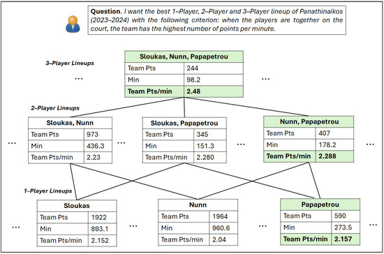
Figure 1.
Running Example—visualization of a semilattice for a question for K-Player lineups.
Furthermore, we can see that for cumulative statistics, such as the number of team points, their value decreases as we visit the supersets, e.g., see the number of minutes of “Sloukas” and “Sloukas, Nunn” nodes in Figure 1. In this way, filtering conditions are easy to execute, i.e., if the condition was the combination of players to have played at least 280 min, then there was no need to compute statistics about any 2,3,4,5-player lineups, including “Papapetrou” (since he has played 273 min in total). On the other hand, it does not hold for the average statistics, e.g., the value of the team points per minute when “Nunn” is on the court is lower than when “Nunn” and “Papapetrou” are on the court.
Regarding our contribution, this paper provides (a) a semilattice-based incremental algorithm that is based on set theory properties for computing the statistics of the restricted power set of the players of a team, (b) comparative results by using a baseline approach and the incremental algorithm, and (c) indicative statistics over the past three EuroLeague seasons and an NBA regular season. Concerning novelty, to the best of our knowledge, this is the first work that tries to compute fast K-Player lineup statistics by using a semilattice approach based on set theory properties.
The rest of this paper is organized as follows: Section 2 discusses the related work, Section 3 introduces the problem statement and the competency questions, and Section 4 describes the steps of the approach and the incremental algorithm. Moreover, Section 5 provides an experimental evaluation, and finally Section 6 concludes the paper and provides directions for future work.
2. Related Work
This section presents related approaches for basketball analytics, then discusses approaches using lattice-based techniques for power set computations, and finally mentions the differences with the related work and the novelty of this paper.
2.1. Basketball Analytics
First, data mining and knowledge discovery techniques have been used for decades for basketball, e.g., see a data mining application for the NBA that was proposed in 1997 [6]. Concerning lineup prediction, the authors in [7] studied the problem of how to choose the best lineup against an opponent team, and they provided graph theory techniques. In [8], a statistical Markov chain model was developed to compare the evolution and performance of players’ positions, to aid the coach in making optimal decisions regarding the player’s rotation line-ups. Moreover, the authors in [9], analyzed and compared statistical data of the NBA and EuroLeague Basketball, and they concluded that EuroLeague “is becoming quantitatively and qualitatively more similar to the NBA”.
In the study of [10], the authors provided a benchmark with existing performance analytics used in the literature for evaluating teams and players, whereas in [11], a framework was introduced for simulating games by calculating different synergies of NBA teams, by comparing their 5-player lineups in several categories. Furthermore, in [12], the authors used a generalized version of Shapley value for evaluating the importance of each player in a given lineup. Also, in [13], a statistical analysis was performed on the historical evolution of the EuroLeague. In addition, the author in [14] exploited dynamic programming techniques, for finding optimal substitution strategies. In addition, there is a benchmark available, called SportQA [15], which contains 70 thousand questions for several sports (including basketball) and can be used for complex analysis.
There are also several works that exploit machine learning techniques for providing basketball analytics. For instance, in [16], the authors exploited machine learning algorithms to predict the winner of European basketball matches, by using over 5000 boxscores, whereas [17] introduced a machine learning framework for predicting the results of NBA games. In addition, ref. [18] surveyed approaches using machine learning algorithms to classify and extract patterns from the movement data of the players. Concerning other data mining techniques in the context of basketball analytics, the authors in [19] exploited association rule mining techniques for uncovering recovery and economic impacts in NBA basketball. Moreover, in [20], such techniques were applied to identify patterns concerning the performance of NBA players quarter-by-quarter.
Furthermore, the authors in [21] used the Shapley additive explanations (SHAP) method for predicting the outcome of an NBA game. SHAP was also exploited in [22] for predicting the next game lineup in collegiate basketball. In particular, SHAP values suggested the important factors for each prediction to aid coaches in making the proper decisions. In addition, ref. [23] proposes a classifier that relies on individual player order statistics for predicting the performance of a five-person basketball lineup. Moreover, ref. [24] introduced counterfactual predictions for evaluating the decision-making skills of players in basketball games.
Regarding the computations of statistics involving combinations of lineups, the official website of the NBA (https://www.nba.com/stats/lineups/traditional, accessed on 15 May 2025) provides statistics over any K-Player combination in tables for the NBA league. Moreover, the website Hack-a-Stat (https://hackastat.eu/en/EuroLeague-stats/, accessed on 15 May 2025) provides Excel files with such statistics for 5-Player lineups for several European Leagues, including EuroLeague. However, there are no details of how they are computed.
2.2. Lattice-Based Measurements over Power Sets
In the past, we have used lattice-based structures for computing content-based measurements in the field of Linked Open Data, i.e., [25]. The objective was to perform several set operations over hundreds of Knowledge Graphs (or datasets), such as to find (i) the intersection of common elements among any combination of datasets in [26], and (ii) the union and complement between the datasets in [27]. Similarly to this paper, we exploited a bottom-up lattice-based approach, which was the fastest one and enabled the computations of millions of combinations in a few seconds.
2.3. Comparison and Novelty
In comparison with the related work, this paper mainly focuses on how to answer fast maximization/minimization questions over any combination of K-Player lineups, instead of trying to predict either the best lineups (e.g., [7]) or the scores of basketball games (e.g., [16,17]). Also, compared to [26,27], we apply lattice-based algorithms to another domain that has different properties. As regards data mining techniques (such as association rules mining [19,20]), we decided to use semilattice structures, since the target is to enable the computation of statistics for any combination of players and not to discover statistically significant patterns in the data that frequently co-occur. On the other hand, these two techniques could be combined, i.e., apply association rule mining to evaluate and prioritize the results of the proposed algorithm based on statistical significance.
Moreover, compared to the website of the NBA, which contains such statistics for any K-Player lineup for the NBA, and the Hack-a-stat website, which provides 5-player lineups statistics for EuroLeague, we focus on the fast computation of the statistics even for maximization and filtering problems. Finally, regarding the novelty, to the best of our knowledge, this is the first work to compute such fast K-Player combination statistics by using a semilattice approach based on set theory properties.
3. Problem Statement and Competency Questions
This section introduces the problem statement and a list of competency questions.
3.1. Problem Statement
The key notations can be seen in Table 1 and are described below.

Table 1.
The key notations of the problem statement and their definitions.
Teams and Players. First of all, we define T as the set of teams , and as all players of a team, i.e., , where .
Power Set of Players of a Team. We define as the power set of any combination of players in a team, i.e., . This power set contains any combination of players, e.g., pairs, triads, quads, quintets, hexads, and so forth.
Restricted Power Set of Players of a Team. The goal is to calculate the statistics for any K-Player combinations of players when they are together on the court. However, since there cannot be more than five players on the court, we restrict the power set to only those subsets that represent legal lineups (e.g., we exclude hexads and so on). Therefore, below, we define the restricted power set of up to combinations of five.
Meet-semilattice. It is a partially ordered set in which every pair of elements has a greatest lower bound (also called the meet, denoted ), which is also in P. The set , together with the subset relation ⊆, forms a meet-semilattice. The meet of any two elements and is given by their intersection, i.e., .
Hasse Diagram. A semilattice can be visualized as a Hasse diagram, which is a graphical representation of a finite partially ordered set . Specifically, each element of P is represented by a node, an edge is drawn between two elements a and b if and there is no such that (i.e., b covers a), and the diagram is drawn so that if , then b appears higher than a in the layout, and edges are directed implicitly upward (edges are not labeled with arrows). An example is given in Figure 1.
Number of Maximum K-Player Combinations. The total number of subsets in is given by summing the binomial coefficients:
For instance, if there are 15 players in a team roster, it results in 3003 5-player combinations, 1365 4-player combinations, 455 3-player combinations, 105 2-player combinations, and 15 1-player combinations, i.e., a total of 4943 combinations.
The 5-player Lineups. Since any time there are lineups of five on the court, we start by defining the lineups having played together for at least 1 s as follows:
All the lineups including a K-Player combination. For a given combination of players, say , we need to find all the 5-player lineups in which they have participated as follows:
How to measure the statistics. We want to compute the team statistics when the combination B is on the court. First, we define as the cumulative number for a given statistic (points, assists, three points made, minutes, etc.) and a combination . The is computed for the desired statistic by taking the sum for for each 5-player lineup that includes all the players of B. For example, for finding all the points of the lineups, including both “Grant” and “Nunn”, we need to take the sum of the points of all the 5-Player lineups, including these two players. Apart from statistics concerning cumulative numbers, there can be statistics, including average values, i.e., . In such cases, we need to combine cumulative statistics to find the average, e.g., for finding the points per minute we need to divide the number of points by the number of minutes .
Set theory Properties. By the given two combinations of players , where it holds that , we know from the set theory that (i.e., see [28]). For instance, if and , we know that the lineups that include “Grant and Nunn” is a superset of the lineups, including “Grant, Nunn, and Sloukas”. Also, if we know that “Lessort and Yurtseven” have never played together, it means that any 3–4 and 5-player combination, including these two players, have never played together in any game. Finally, for the cumulative stats, we know that if , then .
Objective. The objective is to compute any of the statistics of each K-Player combination in an incremental way for exploiting the mentioned set theory properties.
Maximization Questions. One target is to provide an answer to the maximization questions, i.e., give me the combination of players B that maximize the following criteria:
For the first one, an example can be to find which combination of players has the highest plus/minus (when they are on the court); for the second case, it can find which combination of players the team has the highest three-point percentage. Correspondingly, it can be used for minimization problems, e.g., for statistics, such as the number of turnovers, i.e., “give me the K-Player lineups that minimize the number of turnovers”.
Filtering Questions. Another case is to compute filtering questions for a given value F such as , e.g., find all the combinations having played at least 40 min and , e.g., find all the combinations of players that, when they are on the court, the team has over 2 points per minute. In any case, one question can include one or more filtering conditions and one or more maximization/minimization conditions.
3.2. Competency Questions
We provide different types of questions based on their computation, i.e., a set of questions is given below:
[Q1. General Question]: For each K-Player combination of players, give me all the team statistics, when they are on the court.
[Q2. Maximization Question]: With which 3-player combination does the team have the highest number of points per minute?
[Q3. Filtering and Maximization Question]: Give me the best K-Player combination of Panathinaikos, including Kendrick Nunn, that maximizes the value of the 3-Point percentage (extra filtering condition: at least 50 min on the court)?
[Q4. Comparative and Filtering Question]: Compare the best K-Player combinations for all the statistics for the Panathinaikos team for the 2023–2024 and 2024–2025 seasons (that have played together at least 80 min on the court)?
[Q5. Minimization Question]: Give me the top-5 3-player lineups in EuroLeague for the 2023–2024 season that, when they are on the court, the team has the lowest number of opponent points per minute.
[Q6. Distribution Question]: Give me the minutes of each K-Player lineup (for a given K) to check their distribution (e.g., power-law distribution).
4. The Steps and Semilattice Incremental Computations
This section provides the steps for computing the desired metrics, the traversal that is used by the algorithms, a baseline method, the proposed incremental algorithm, and how it can be adjusted for questions requiring some maximization and/or filtering conditions.
4.1. The Steps and the Focus of This Paper
We present the steps and the focus of this paper, which are also depicted in Figure 2.
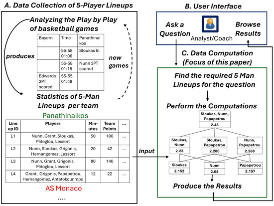
Figure 2.
The steps and the focus of this paper.
Data Collection. The first step includes the analysis of the play-by-play for the desired games (left part of Figure 2). The target is to collect all the statistics for all 5-player lineups (i.e., ) that have played together (at least one second) for each team. As a result, we have all the statistics for all the 5-player lineups of each team. Certainly, in that step, one can exclude specific lineups/games, e.g., to collect only the home or away games, the games that the team won or lost, the lineups in the last quarter, etc. Since more and more games are played as time passes in a single season, the 5-player lineups should be updated. In the example of Figure 2, we can see such 5-player lineups for a given team and some indicative statistics (minutes, points).
User Interface and Data Computation. The user, e.g., a data analyst, a coach, can express a question (see the upper right part of Figure 2) to conduct an analysis for a single team and/or several teams. The main notion is that the algorithm finds the desired 5-player lineups (and statistics) based on the given question and uses them as input for the computations. For instance, if the question is about all the teams, e.g., “Give me the K-Player lineup of each team that maximizes the number of assists per 40 min”, then the algorithm will perform separately the computation for each team and will produce the results, which are finally returned to the user.
Focus of this paper. The focus of this paper is the computation phase, i.e., the effective computation of the measurements of any K-Player combination based on precomputed 5-player lineup statistics. For this reason, we use existing precomputed statistics for all 5-player lineups of all teams that are available in the Hack-a-stat and NBA websites. We have stored them in TSV (Tab-Separated Values) format, and we update them periodically. On the other hand, the ultimate target is to extend this work by analyzing the play-by-play from existing APIs and updating the statistics (even in real time), e.g., for EuroLeague, this can be completed through the EuroLeague API (https://live.euroleague.net/api/PlaybyPlay?gamecode=333&seasoncode=E2023, accessed on 15 May 2025). In this way, we expect to have such an analysis even during a given game, e.g., at half-time, since for the time being, we do not handle dynamic updates. Finally, we plan to provide an interactive user interface to analysts/coaches for expressing their questions by enabling the selection of specific teams, players, etc.
4.2. The Depth-First Search Traversal
For the algorithms (including the baseline), we follow a Depth-First Search (DFS) traversal. An example with all the combinations of four players is depicted in Figure 3. The figure shows the visiting order (with red color). We always go upwards, and we never visit a combination of players twice. We can clearly see that we first compute all the combinations, including “Nunn”, then all the combinations, including “Grant” (but without “Nunn”, since they have been computed previously), and so forth. Due to this traversal, we can visit and compute the metrics for any K-Player combination at run time. This means that we do not pre-construct a data structure for the lattice. Finally, it allows us to stop the computation at any K.
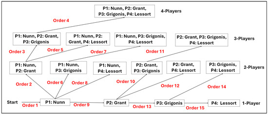
Figure 3.
The (Depth-First Search) DFS traversal for 4 players.
4.3. Baseline Method
For the baseline, we follow the mentioned DFS traversal for a given team. In particular, we start from the bottom, and for each subset , we iterate over each . For each iteration, we check if and only if it holds, we take the sum of the desired cumulative statistic(s), and in the end, we can compute the average statistics.
Example of the Baseline. Suppose that we perform the traversal of Figure 3 for computing all the metrics by using as input the collected 5-player Lineups that are depicted on the left lower side of Figure 2. Thereby, we will start from “Nunn”, and we will check for each of the four 5-player lineups (of Figure 2) if they contain “Nunn”. Afterwards, we will visit the pair “Nunn, Grant”, and we will check again for each of the four 5-player lineups if they contain both “Nunn” and “Grant”. Generally, we perform the same process for each K-Player lineup of the given team.
Time and Space Complexity. In this way, we need each K-Player combination to check each 5-player lineup of the team, i.e., we need iterations, and the time complexity is (). Although it can be expensive to compute the statistics for all the K-Player lineups, this method is suitable for answering questions for a single Player combination, e.g., give me all the statistics when the players {Nunn, Hernangomez, Lessort} are on the court. The space complexity is .
4.4. Semilattice-Based Incremental Algorithm
The problems with the baseline model are that (a) we need to iterate over all the for each K-Player combination, (b) we can even perform computations for combinations that have never played together, and (c) we do not reuse statistics, which is important for some queries, e.g., for the cumulative statistics, we know that if , then and also .
Input. The algorithm (see Algorithm 1) uses as input post-match static data. Specifically, it receives as parameters the players of a team, a number i to know the order of the players, the current combination of players B, and the 5-player lineups, including all the players of B, i.e., .
| Algorithm 1: Semilattice incremental computation of statistics for all K-Player lineups () |
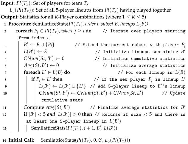 |
Initial Call. First, we call the function (see line 14) with the following parameters: , i.e., all the players of the desired team, , i.e., to start from the first player, the emptyset (), since we start from the bottom. We also give all the 5-player lineups of the team that have played together at least 1 s.
Procedure. We start from the bottom, iterate over the players of the team, add in our current K-Player combination the player , and initialize some variables (lines 3–6). Afterwards, we iterate over all the lineups , and we check if the players of our current lineup exist in each 5-player lineup. If it is true, we add the 5-player lineup to the lineups of , and we increase the value of the cumulative statistics (lines 7–10). For instance, if the first player is “Nunn”, then we keep each 5-player lineup, including “Nunn”. After having computed the cumulative statistics, we can also compute the average statistics (if we desire), i.e., line 11.
Recursion. The next step is to continue upwards in a recursive way (lines 11–13). We increase the value of i, we “transfer” the lineups of the current combination since we know from the set theory that if , then . Therefore, in the next recursion, a new player will be added to the combination, and we will perform the same computations by reusing the from the previous lineup. If our combination of players reaches 5, there is no need to continue upwards and compute any statistics (there cannot be more than 5 players on the court); thereby, we return to the previous level (recursively). Moreover, if we do not find any lineups , including the combination , there is also no need to continue upwards.
Example of the Incremental Algorithm. In Figure 4, we perform the computations for any combination of four players of a given team. The task is to compute the total team points when any K-Player lineup (of these players) is on the court. As an input, we use the statistics from the 5-player lineups (see the bottom part of Figure 4). We start from “Nunn”, we find in which 5-player lineups he has participated in, and we compute the statistics. Indeed, “Nunn” was part of the lineups with IDs , and the sum of the team points in these lineups was 282 points.
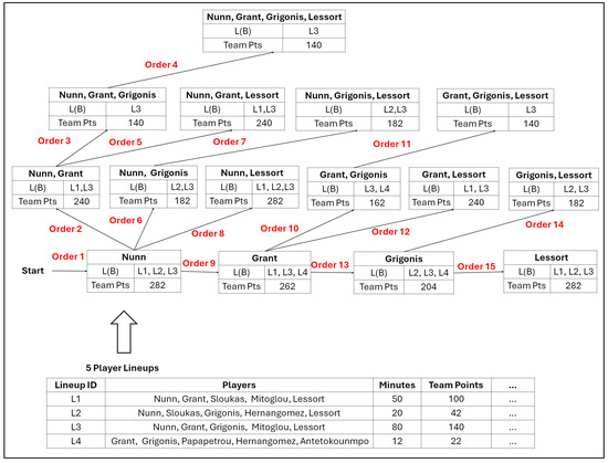
Figure 4.
The semilattice depth-first search traversal for a subset of players—the task is to find the number of team points when the players are on the court.
The next step is to continue upwards, by transferring and by adding a new player, e.g., “Grant” (line 3 of Algorithm 1). We iterate only over the lineups, including “Nunn”, and if they also include “Grant”, we keep them (see for that pair of players) and we use them to compute the statistics (lines 7–10 of Algorithm 1). Therefore, the difference in our example with the baseline algorithm is that for the baseline, we needed to iterate over all four lineups to check if “Nunn” and “Grant” were part of each 5-player lineup. On the contrary, here, we iterate over the three lineups, including “Nunn” (with IDs ), and we check if Grant is part of each of these lineups (i.e., he is part of lineups with IDs ). In this way, as we go upwards, the size of decreases, e.g., when we reach the top node, we perform a check only for one 5-player lineup (i.e., ). In the end, the final result is that we have computed the total team points for each combination.
Time and Space Complexity. Since we follow a DFS, in the worst case (where any combination of players have played together for at least one second), we visit each node (combination of players) once, and we create one edge per K-Player combination, i.e., . For each combination of players , we iterate over entries for finding the . Therefore, the time complexity here is (), where denotes the average number of that we need to iterate for finding the 5-player lineups for each K-Player combination. Concerning space complexity, it is , where are the subsets that occur in the maximum depth d of the lattice (maximum is 5 in our case).
4.5. Filtering, Maximization, and Order of Players
Here, we discuss how the algorithm can be adjusted for filtering, maximization/minimization, and we discuss the visiting order of players.
Filtering and Maximization/Minimization. In Algorithm 1, in line 11, we can add code to keep the maximum or minimum values, e.g., to find the , the , etc. Regarding filtering, we can perform more checks in line 12. For example, we can stop at any K (e.g., triads of players), and we can keep the maximum/minimum or the top-X values (e.g., top-10). Also, we can stop if a cumulative statistic is higher/lower than a given value, e.g., , to compute the statistics only for K-Player lineups that have played at least 40 min together, and so forth. In this way, fewer nodes (K-Player combinations) will be visited. As an example, in Figure 4, in case we desire K-Player combinations with at least 200 team points, there is no need to visit the quad of players since we already know that when “Nunn, Grant, Grigonis” were on the court, the team scored less than 200 points.
Is the order of players important? Since we transfer of a given B to , the order of players can be of primary importance. As an example in Figure 5, we can see the computations of the AS Monaco players. In the lower part, we observe that “James” occurs in five 5-player lineups, “Theis” in three, and “Jaiteh” in one. In the upper left side, we use a descending order regarding the number of 5-player lineups per player. Thus, we start with “James”, and then by visiting “James, Theis”, we transfer five 5-player lineups and we keep only the three 5-player lineups, including both players. Then, we visit the triad of players, and we transfer the three 5-player lineups; however, since this triad of players have never played together, the is empty. Generally, with that order, we visit all the nodes, and we transferred, in total, 16 5-player lineups. Therefore, more iterations are needed in line 7 of Algorithm 1. On the upper right side, for the same players, we follow an ascending order. We start from “Jaiteh”, and since he has participated only in one 5-player lineup, we transferred that lineup to the pair “Jaiteh, Theis”. However, since these two players have never played together (they are both Centers), and is empty, we do not need to visit the triad of players. By using this order, we visited fewer nodes and performed fewer iterations.
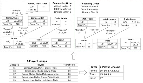
Figure 5.
An example for the ascending versus descending order with respect to the number of 5-player lineups per player for the semilattice incremental algorithm.
In the experiments, we evaluate different orders of players, i.e., an ascending order (e.g., right part of Figure 5), a descending order (e.g., left part of Figure 5), and a random order. For each order, we provide results about a) the number of visited nodes (K-Player combinations) and b) the number of the total and average iterations, i.e., to find .
5. Experimental Evaluation
We first provide some details for the datasets and the experimental setup, then we discuss comparative results on the algorithms, and we present some indicative statistics on the lineups. Finally, we provide a discussion and specific research directions.
5.1. Datasets
Since we focus on EuroLeague, we use the 5-player lineups from EuroLeague 2022–2023, 2023–2024, and 2024–2025 (until the regular season since it is an ongoing season) from Hack-a-Stat (https://hackastat.eu/en/EuroLeague-stats/, accessed on 15 May 2025). Moreover, we manually collected all the 5-player Lineup statistics for the NBA regular season 2023–2024 from the NBA website (https://www.nba.com/stats/lineups/traditional, accessed on 15 May 2025) since we wanted to also perform the measurements in a larger dataset, i.e., NBA contains 30 teams and they play over 1200 games per season, while the EuroLeague includes 18 teams, and the number of games is approximately 330.
The initial datasets are in .tsv format (tab separated values), and an overview is provided in Table 2. The initial datasets contain only the statistics of the 5-player lineups. Also, in that table, for each , we see the number of combinations that have played together for each season for all the teams (computed using the algorithms presented in this paper). In the NBA, there are approximately more K-Player lineups than in the EuroLeague.
Table 2.
Datasets used in the experiments and the distinct number of K-Player lineups. For , the statistics were derived after the computations using the proposed algorithm.
5.2. GitHub Page, Software, and Hardware
The GitHub page (https://github.com/mountanton/Basketball_K-Player_Lineups, accessed on 15 May 2025) contains the input files and the output files with all the statistics for all the K-Player combinations of EuroLeague for the 2022–2023, 2023–2024, and 2024–2025 seasons.
Software. The GitHub page also provides the code which has been written in JAVA programming language. The current version of the code enables the user to run the experiments for the datasets of Table 2. The users can test all the methods for computing the statistics for all the K-Player combinations. Also, it has an example for a maximization and filtering query to compute the best K-Player lineup having the most points per minute.
Hardware. For all the experiments, we use a single machine having an i5 core, 16 GB main memory, and 500 GB disk space.
5.3. Experimental Setup
First, for the efficiency measurements, we provide the execution time for the general competency question Q1. In particular, we compute a set of 38 key cumulative and average statistics for all the combinations of players of all the datasets by using (a) the baseline model (described in Section 4.3) and (b) the semilattice incremental method (described in Section 4.4). For the semilattice method, we provide results with a different order of players: (b1) semilattice (asc), i.e., an ascending order according to the number of lineups that the players of a team have participated in (e.g., if a player has participated in the fewer lineups, we will start from player X), (b2) semilattice (desc), i.e., the opposite of the previous one, and (b3) semilattice (rand), i.e., a random order of players.
We have performed 10 independent runs for each method to account for variability in execution time and ensure statistical robustness. We provide the following results for each dataset: (i) average execution time per method, (ii) p-value (statistical significance) between each pair of methods, and (iii) number of visited nodes and iterations per method. Finally, we provide an example for the competency questions Q2 to Q6.
5.4. Efficiency Results
Execution Time per Method. We can see the average execution time per method (average for the 10 runs) for each EuroLeague season in Figure 6. The semilattice methods are much faster than the baseline one for all the EuroLeague seasons. Indeed, we managed to compute all the statistics for all the K-Player combinations of players () very fast, e.g., on average, 0.67 s for the 2023–2024 season, whereas for the baseline method, we needed 19.35 s, i.e., 28.61× faster. Concerning the other seasons, for 2022–2023, the semilattice (asc) method was faster, and for 2024–2025, it was faster. As regards NBA, Figure 7 shows that the difference is much higher, i.e., we computed the statistics, on average, in 2.11 s, whereas for the baseline, we needed 488 s, i.e., 230× faster. Moreover, Figure 8 and Figure 9 show the execution time per run, for the Euroleague 2023–2024 and for NBA regular season 2023–2024. Generally, the execution time for the semilattice methods is more stable, whereas the baseline shows a higher variance in execution time.
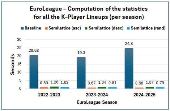
Figure 6.
Average execution time (10 runs) for all the K-Player combinations of players (EuroLeague).
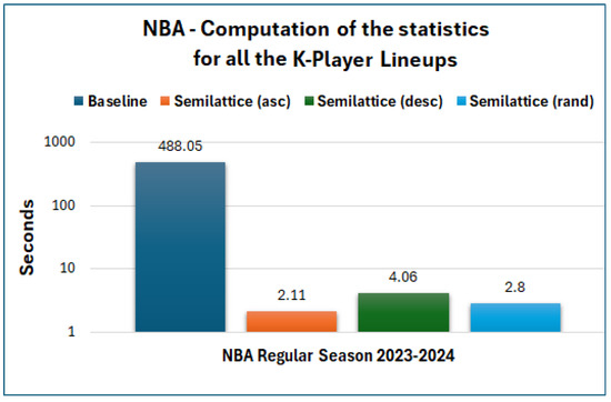
Figure 7.
Average execution time (10 runs) for all the K-Player combinations of players—NBA regular season 2023–2024.
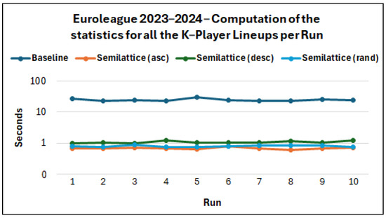
Figure 8.
Execution time per run for each method for Euroleague 2023–2024 (log-linear plot).
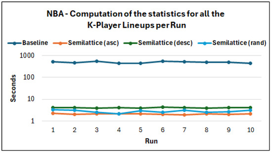
Figure 9.
Execution time per run for each method for NBA 2023–2024 (log-linear plot).
Statistical significance (p-values). Table 3 shows the statistical significance between the method pairs. Specifically, the paired t-tests conducted on execution times across the three EuroLeague seasons, as well as the NBA dataset, show that all method pairs exhibit statistically significant differences in performance ( in every comparison). Specifically, we observe highly significant performance differences between the baseline and the semilattice methods.
Table 3.
Paired t-test p-values comparing execution times between baseline (BS) and semilattice methods across EuroLeague (EL) seasons and the NBA dataset.
Visited nodes and iterations per method. This time difference is important for real-time queries and can be explained by checking Table 4 and Table 5 for the EuroLeague and NBA, respectively (for 2023–2024 season). The main reason is that for the baseline method, we need to check all the possible K-Player combinations (since it does not exploit set theory properties), and we need to iterate each time over all the 5-player lineups of a team for each K-Player combination. More specifically, for the baseline, we needed EuroLeague (2023–2024) to check 153 thousand K-Player combinations and perform over 5 million iterations to find the . In contrast, by using the semilattice (asc) method, we managed to compute the statistics by visiting 48 thousand K-Player combinations by performing only 57 thousand iterations (i.e., 7.8 per K-Player combination). Regarding the regular 2023–2024 NBA season, where more teams and lineups are included, the difference is much higher, and it is worth mentioning that for the baseline method, we needed to visit over 1.5 million K-Player combinations and perform over 1 billion iterations.
Table 4.
Comparative results for computing the statistics for all K-Player combinations of all EuroLeague Teams—2023–2024 season. Bold text indicates the lowest numbers.
Table 5.
Comparative results for computing the statistics for all the K-Player combinations of all NBA teams—2023–2024 regular season. Bold text indicates the lowest numbers.
Comparison of semilattice methods. The ascending order of players (e.g., starting from the player with the fewest number of minutes on the court) was the most effective one, i.e., on average, faster than the descending order and faster than a random order. For all the semilattice orders, we needed, on average, fewer iterations per combination; however, for the random and descending one, we visited much more lattice nodes (i.e., K-Player combinations), i.e., see Table 4 and Table 5.
5.5. Indicative Statistics for Competency Questions—EuroLeague
Here, we provide some indicative statistics for the remaining competency questions as follows: (Q2) the best 3-player combination of players in each team with the highest number of points per minute (season 2023–2024) for K-Player combinations having played at least 80 min on the court, (Q3) the best K-Player combination including “K. Nunn” that maximizes the 3-point percentage, (Q4) the best K-Player combination of Panathinaikos for a set of 10 statistics for the 2023–2024 and 2024–2025 seasons (regular season), (Q5) the top-5 3-player lineups with the lowest number of opponent points per minute (at least 50 min on the court) for the 2023-2024 season, and (Q6) checking for power-law distribution for the minutes of K-Player lineups (EuroLeague 2023–2024 season).
Question Q2. Table 6 shows the results for Q2, for all the EuroLeague teams, and the highest number of points per minute achieved by the triad of players {Campazzo, Causeur, Deck} of Real Madrid with 2.54 points per minute.
Table 6.
The best 3-player combination of each team giving the team the highest number of points per minute (EuroLeague 2023–2024). Bold text indicates the best combination.
Question Q3. From the measurements, we found that the best K-Players for the given question (2023–2024 season) was {Nunn, Sloukas, Papapetrou, Mitoglou} with a 3-point percentage 53.1%, i.e., when these four players were on the court, the team had 17 out of 32 that made three-points shots. Regarding the 2024–2025 season, the best K-Player group was {Nunn, Grant, Sloukas, Mitoglou} with a 3-point percentage of 49.2% (32 out of the 65).
Question Q4. From Table 7, we can observe that for the 2023–2024 season, J. Grant was a key player of Panathinaikos for most of the categories, both on offense and defense, whereas for the 2024–2025 season (ongoing, regular season), when “J. Grant, J. Hernangomez, and P. Kalaitzakis” are on the court, the team seems to be effective in many categories, such as the number of rebounds per minute and the performance index rating.
Table 7.
The best K-Player combination, where Panathinaikos achieves the best values when the players are on the court at least 80 min.
Question Q5. Table 8 provides the top-5 3-player lineups (2023–2024 season), with the lowest opponent points per minute, and as we can see, the top triad of players allowed only 1.32 points per minute for the opponents.
Table 8.
The top-5 best 3-player combinations in the 2023–2024 season with less opponent points per minute.
Question Q6. In Figure 10, we can clearly observe a power-law distribution for the minutes played of the K-Player lineups in EuroLeague, for every K in the range . It is worth mentioning that half of the 5-player lineups played together less than 2 min in the whole season.
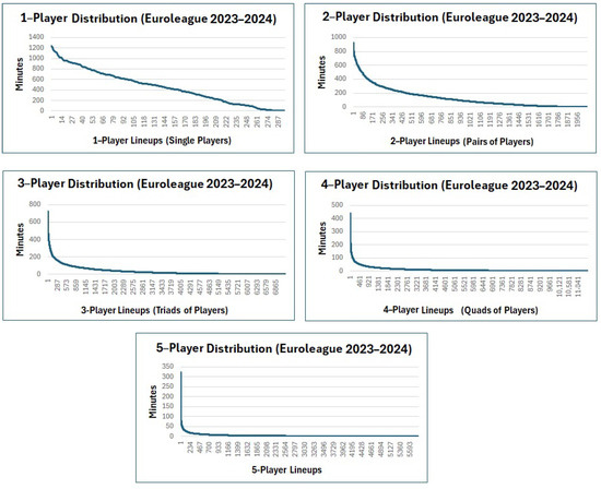
Figure 10.
K-Player distributions in EuroLeague 2023–2024 (having played together at least 1 s).
5.6. Discussion, Limitations, and Future Directions
By using the semilattice approach, we managed to answer the research questions RQ1 and RQ2, i.e., for RQ1, we exploited set theory properties through the semilattice methods for reusing previous measurements, whereas for RQ2, we managed to compute the statistics very fast, i.e., in 2.1 s for the NBA and less than 1 s in the EuroLeague, which is of primary importance for real-time questions. Moreover, the difference was high compared to a baseline approach, i.e., it was even more than 200× faster. Certainly, for many questions, there is no need to compute all the statistics and visit all the nodes, e.g., for the competency question Q3, we need to compute the metrics only for Panathinaikos and only for the lineups including “Nunn”.
Regarding limitations which are targets of future work, at the time being, we use existing post-match 5-player lineups statistics, and we do not collect them in real time. Moreover, although the code is provided and offers some basic scenarios, there is no available interactive web interface. Thereby, the target is to automate the whole process by collecting statistics automatically by creating a crawler and offer an interactive web application that provides real-time answers, by providing the opportunity to the user to ask different types of questions (e.g., like the Competency Questions). One other direction is to use and/or create a Knowledge Graph for enabling the expression of more advanced questions, e.g., “Give me the statistics of lineups including at least three players with height over 2.05” since we can retrieve the height of each player from a KG (and any desired information, like age, college, position, NBA draft number, etc.). Another interesting direction could be to provide measurements for analyzing the performance of a specific player in a given K-Player lineup, e.g., “In which 3-player lineup, did Kendrick Nunn maximize his 3-point percentage?”. Such a question requires each 5-player Lineup to keep the exact statistics for each of the players in the lineup, which can also be done in the case of creating our own crawler.
6. Concluding Remarks
In this paper, we presented a semilattice algorithm for computing the team statistics of a basketball team, when any K-Player combination of players is on the court (). The algorithm exploits set theory properties and follows a depth-first search traversal, for reusing computations of lineups, and is essential for maximization/minimization and filtering problems, e.g., for finding which K-Player lineup maximizes a given statistic. Regarding the experiments, we used real datasets from EuroLeague and NBA, and indicatively we managed to compute in 0.67 s a key set of statistics for all the K-Player combinations that have played together in EuroLeague (2023–2024) and in 2.1 s for the NBA regular season (2023–2024). Compared to a baseline method, the proposed algorithm was more than faster for the computations for the NBA and over faster for the EuroLeague. Finally, we presented indicative statistics for the EuroLeague.
As future work, we plan to (a) use a crawler to analyze the play-by-play of each game, e.g., for including/excluding specific games and for providing more advanced statistics (even in real time), (b) create a user-friendly web application for enabling the fast answering of any maximization/minimization or/and filtering questions by using the proposed algorithms, (c) create an ontology and a knowledge graph for enabling the execution of more complex queries regarding the statistics, boxscores, and play-by-play of basketball games, and (d) use the same incremental algorithm in other sports.
Funding
This research received no external funding.
Institutional Review Board Statement
Not applicable.
Informed Consent Statement
Not applicable.
Data Availability Statement
All the datasets of this study, experimental results, and code for running the experiments are available in https://github.com/mountanton/Basketball_K-Player_Lineups, accessed on 15 May 2025.
Conflicts of Interest
The authors declare no conflicts of interest.
References
- Singh, N. Sport analytics: A review. Learning 2020, 9, 64–69. [Google Scholar] [CrossRef]
- Ghosh, I.; Ramasamy Ramamurthy, S.; Chakma, A.; Roy, N. Sports analytics review: Artificial intelligence applications, emerging technologies, and algorithmic perspective. Wiley Interdiscip. Rev. Data Min. Knowl. Discov. 2023, 13, e1496. [Google Scholar] [CrossRef]
- Piette, J.; Pham, L.; Anand, S. Evaluating basketball player performance via statistical network modeling. In Proceedings of the 5th MIT Sloan Sports Analytics Conference, Boston, MA, USA, 4–5 March 2011; pp. 4–5. [Google Scholar]
- Devlin, S.; Uminsky, D. Identifying group contributions in NBA lineups with spectral analysis. J. Sport. Anal. 2020, 6, 215–234. [Google Scholar] [CrossRef]
- Vinué, G.; Epifanio, I. Archetypoid analysis for sports analytics. Data Min. Knowl. Discov. 2017, 31, 1643–1677. [Google Scholar] [CrossRef]
- Bhandari, I.; Colet, E.; Parker, J.; Pines, Z.; Pratap, R.; Ramanujam, K. Advanced scout: Data mining and knowledge discovery in NBA data. Data Min. Knowl. Discov. 1997, 1, 121–125. [Google Scholar] [CrossRef]
- Ahmadalinezhad, M.; Makrehchi, M.; Seward, N. Basketball lineup performance prediction using network analysis. In Proceedings of the IEEE/ACM International Conference on Advances in Social Networks Analysis and Mining, Vancouver, BC, Canada, 27–30 August 2019; pp. 519–524. [Google Scholar] [CrossRef]
- Kolias, P.; Stavropoulos, N.; Papadopoulou, A.; Kostakidis, T. Evaluating basketball player’s rotation line-ups performance via statistical markov chain modelling. Int. J. Sport. Sci. Coach. 2022, 17, 178–188. [Google Scholar] [CrossRef]
- Mandić, R.; Jakovljević, S.; Erčulj, F.; Štrumbelj, E. Trends in NBA and Euroleague basketball: Analysis and comparison of statistical data from 2000 to 2017. PLoS ONE 2019, 14, e0223524. [Google Scholar] [CrossRef]
- Sarlis, V.; Tjortjis, C. Sports analytics—Evaluation of basketball players and team performance. Inf. Syst. 2020, 93, 101562. [Google Scholar] [CrossRef]
- Maymin, A.; Maymin, P.; Shen, E. NBA chemistry: Positive and negative synergies in basketball. Int. J. Comput. Sci. Sport 2013, 12, 4–23. [Google Scholar] [CrossRef]
- Metulini, R.; Gnecco, G. Measuring players’ importance in basketball using the generalized Shapley value. Ann. Oper. Res. 2023, 325, 441–465. [Google Scholar] [CrossRef]
- Katris, C. Exploring Euroleague History using Basic Statistics. arXiv 2023, arXiv:2301.02443. [Google Scholar]
- Hughes, D.W. An Approximate Dynamic Programming Approach to Determine the Optimal Substitution Strategy for Basketball. Ph.D. Thesis, George Mason University, Fairfax, VA, USA, 2017. [Google Scholar]
- Xia, H.; Yang, Z.; Wang, Y.; Tracy, R.; Zhao, Y.; Huang, D.; Chen, Z.; Zhu, Y.; Wang, Y.; Shen, W. Sportqa: A benchmark for sports understanding in large language models. arXiv 2024, arXiv:2402.15862. [Google Scholar]
- Lampis, T.; Ioannis, N.; Vasilios, V.; Stavrianna, D. Predictions of European basketball match results with machine learning algorithms. J. Sport. Anal. 2023, 9, 171–190. [Google Scholar] [CrossRef]
- Thabtah, F.; Zhang, L.; Abdelhamid, N. NBA game result prediction using feature analysis and machine learning. Ann. Data Sci. 2019, 6, 103–116. [Google Scholar] [CrossRef]
- Stephanos, D.K.; Husari, G.; Bennett, B.T.; Stephanos, E. Machine learning predictive analytics for player movement prediction in NBA: Applications, opportunities, and challenges. In Proceedings of the ACM Southeast Conference, Virtual, 15–17 April 2021; pp. 2–8. [Google Scholar] [CrossRef]
- Sarlis, V.; Papageorgiou, G.; Tjortjis, C. Leveraging Sports Analytics and Association Rule Mining to Uncover Recovery and Economic Impacts in NBA Basketball. Data 2024, 9, 83. [Google Scholar] [CrossRef]
- Iatropoulos, D.; Sarlis, V.; Tjortjis, C. A Data Mining Approach to Identify NBA Player Quarter-by-Quarter Performance Patterns. Big Data Cogn. Comput. 2025, 9, 74. [Google Scholar] [CrossRef]
- Ouyang, Y.; Li, X.; Zhou, W.; Hong, W.; Zheng, W.; Qi, F.; Peng, L. Integration of machine learning XGBoost and SHAP models for NBA game outcome prediction and quantitative analysis methodology. PLoS ONE 2024, 19, e0307478. [Google Scholar] [CrossRef]
- Sharma, S.; Divakaran, S.; Kaya, T.; Raval, M. Athletic signature: Predicting the next game lineup in collegiate basketball. Neural Comput. Appl. 2024, 36, 21761–21780. [Google Scholar] [CrossRef]
- Martonosi, S.E.; Gonzalez, M.; Oshiro, N. Predicting elite NBA lineups using individual player order statistics. J. Quant. Anal. Sport. 2023, 19, 51–71. [Google Scholar] [CrossRef]
- Fujii, K.; Takeuchi, K.; Kuribayashi, A.; Takeishi, N.; Kawahara, Y.; Takeda, K. Estimating counterfactual treatment outcomes over time in complex multiagent scenarios. arXiv 2024, arXiv:2206.01900v4. [Google Scholar] [CrossRef]
- Mountantonakis, M. Services for Connecting and Integrating Big Numbers of Linked Datasets; IOS Press: Amsterdam, The Netherlands, 2021; Volume 50. [Google Scholar] [CrossRef]
- Mountantonakis, M.; Tzitzikas, Y. On measuring the lattice of commonalities among several linked datasets. Proc. VLDB 2016, 9, 1101–1112. [Google Scholar] [CrossRef]
- Mountantonakis, M.; Tzitzikas, Y. Content-based union and complement metrics for dataset search over RDF knowledge graphs. J. Data Inf. Qual. (JDIQ) 2020, 12, 1–31. [Google Scholar] [CrossRef]
- Hrbacek, K.; Jech, T. Introduction to Set Theory, Revised and Expanded; CRC Press: Boca Raton, FL, USA, 2017. [Google Scholar] [CrossRef]
Disclaimer/Publisher’s Note: The statements, opinions and data contained in all publications are solely those of the individual author(s) and contributor(s) and not of MDPI and/or the editor(s). MDPI and/or the editor(s) disclaim responsibility for any injury to people or property resulting from any ideas, methods, instructions or products referred to in the content. |
© 2025 by the author. Licensee MDPI, Basel, Switzerland. This article is an open access article distributed under the terms and conditions of the Creative Commons Attribution (CC BY) license (https://creativecommons.org/licenses/by/4.0/).