A Personalized Itinerary Recommender System: Considering Sequential Pattern Mining

Abstract

Personalized itinerary recommendations are essential as many people choose traveling as their primary leisure pursuit. Unlike model-based and optimization-based methods, sequential-pattern-mining-based methods, which are based on the users’ previous visiting experience, can generate more personalized itineraries and avoid the difficulties caused by the two methods. Although sequential-pattern-mining-based methods have shown promise in generating personalized itineraries, the following three challenges remain. First, they often overlook user diversity in time and category preferences, leading to less personalized itinerary suggestions. Second, they typically evaluate sequences only by POI preference, ignoring crucial factors of optimal visiting times and travel distance. Third, they tend to recommend feasible but not optimal itineraries without exploring extended combinations that could better meet user constraints. To solve the difficulties above, a novel personalized itinerary recommendation system for social media is proposed. First, the user preference, which contains time and category preferences, is generated for all users. Users with similar preferences are clustered into the same group. Then, the sequential pattern mining algorithm is adopted to create frequent sequential patterns for each group. Second, to evaluate the suitability of an itinerary, we define the itinerary score according to the considerations of the POI preference, time matching, and travel distance. Third, based on the tentative itineraries generated from the sequential pattern mining process, the Sequential-Pattern-Mining-based Itinerary Recommendation (SPM-IR) algorithm is developed to create more candidate itineraries under user-specified constraints. The top-N candidate sequences ranked by the proposed itinerary score are then returned to the target user as the itinerary recommendation. A real-life dataset from geotagged social media is implemented to demonstrate the benefits of the proposed personalized itinerary recommendation system. Empirical evaluations show that 94.82% of the generated itineraries outperformed real-life itineraries in POI preference, time matching, and travel-distance-based itinerary scores. Ablation studies confirmed the contribution of time and category preferences and highlighted the importance of time matching in itinerary evaluation.

1. Introduction

The latest World Tourism Barometer from UN Tourism reported that international tourism experienced a significant resurgence in 2024, with an estimated 1.4 billion tourists traveling abroad. This figure represents a near-complete recovery of pre-pandemic levels, achieving 99% of the 2019 benchmark. The increase of 11% over 2023, or an additional 140 million international tourist arrivals, was primarily driven by robust post-pandemic demand, strong performance from major source markets, and the continued recovery of destinations in Asia and the Pacific [1]. While online travel blogs, tourism-focused Q&A platforms, and search engines provide scattered Points of Interest (POIs), these suggestions often fail to align with individual preferences [2,3]. Various model-based approaches, such as next-location, top-k location, and travel region recommendations, have been proposed to enhance travel recommendations [4,5,6,7]. Next-location recommendation techniques predict subsequent POIs based on users’ prior trajectories, while top-k location recommendations present a selection of appealing POIs. Although these approaches accurately predict user preferences for individual POIs, they struggle to generate complete itineraries that accommodate personalized constraints, such as designated start/end locations and travel time limitations [8,9,10].

To incorporate multiple constraints, itinerary planning has been formulated as variants of the orienteering problem (OP) or traveling salesman problem (TSP), employing optimization techniques to generate recommended itineraries [11,12]. For example, reference [3] formulated tour recommendation as an orienteering problem, addressing time limits and fixed-POI constraints via PERSTOUR, prioritizing POI popularity and user preferences derived from trajectories. Reference [13] extended classical orienteering by introducing OPFP, where node scores depend on route context and inter-node relationships. Reference [2] proposed DCC-PersIRE, combining unsupervised deep learning for POI embeddings with ILS-based optimization to balance user interest and POI popularity within time budgets. These methods aim to arrange POIs into itineraries that maximize tourist satisfaction while adhering to temporal and spatial constraints. However, accurately capturing user interests remains challenging.

Despite advancements in model-based and optimization-based methods, model-based methods need to find the best parameter set to achieve high prediction accuracy [14,15], while optimization approaches must set up many constraints and might generate unreasonable answers [2,16]. Unlike the two methods, sequential pattern mining, which is based on the users’ previous visiting experience, can generate personalized itineraries and avoid the problems caused by the two methods. For instance, Reference [17] proposed a touring path suggestion system that utilizes previous popular visiting trajectories and a time-interval sequential pattern mining algorithm to generate personalized tours. Reference [18] introduced the Location-Item-Time (LIT) sequence to describe spatial and temporal behavior in theme parks, developing the LIT PrefixSpan algorithm to discover frequent LIT patterns. They also proposed a route suggestion procedure to retrieve suitable patterns based on visitor preferences, such as time constraints and favorite items. Reference [19] proposed a novel approach to integrating diverse website tourism data, creating a comprehensive POI knowledge base and structured POI visit sequences. A POI-Visit sequential pattern mining algorithm is developed to generate fine-grained candidate POI routes, incorporating various tourism contexts. The system then retrieves and ranks these routes based on the querying tourist’s specific contexts, such as travel duration, companion type, visit season, and preferred POI types.

Although sequential pattern mining is increasingly used for personalized itinerary recommendations, the current approaches still face three challenges that hinder their practical effectiveness. First, they often rely on a single social media dataset and ignore key variations in users’ time and category preferences. For example, older people like to travel in the early morning, while young people prefer to travel in the afternoon. In addition, family tourists prefer theme parks, while single tourists prefer museums. Ignoring the difference between the users’ time and category preferences makes the generated candidate sequence unsuitable for the target user. Second, most systems evaluate itinerary quality solely based on POI preferences, overlooking crucial factors such as optimal visiting times and travel distance, significantly affecting a tour’s feasibility and comfort [2,3,14]. For example, suppose the best visiting time for A is 10:00, and that for B is 12:00. In that case, the sequence A–B should be a better choice than the sequence B–A if the start visiting time is 10:00. Third, previous studies generate sequence suggestions based on their tailored sequential pattern mining methods. Although these methods can effectively create a set of sequence suggestions, most are feasible but not near-optimal solutions [20]. For example, if A–D–B, B–E–C, and A–B–C are sequences generated from sequential-pattern-mining-based methods, previous studies might suggest one of them if one’s support value is the largest. However, it should be worthwhile to try sequences of A–D–B–C and A–B–E–C to see if they can satisfy the constraints provided by the user. Exploring the possible sequences from the generated sequences should be worthwhile to obtain a better suggestion result. Addressing these challenges is critical for enhancing the accuracy of recommendations and improving tourists’ satisfaction, optimizing time use, and encouraging deeper engagement with destination experiences.

To address these limitations, we propose a novel personalized itinerary recommendation system. First, to address the issue that users on the social media platform are different, the user preference, which contains time and category preferences, is generated for all users. Users with similar preferences are clustered into the same group. Then, the sequential pattern mining algorithm is adopted to create frequent sequential patterns for each group. Second, to evaluate the suitability of an itinerary, we define the itinerary score according to the following three considerations: POI preference score, time-matching score, and travel distance score. The POI preference score evaluates how the user likes the POIs in the itinerary, which is determined by the POI popularity and the POI attractiveness of the itinerary. The time-matching score evaluates whether the expected arrival time to visit POIs in the itinerary is suitable. The travel distance score considers how the itinerary’s travel distance affects the user’s choice. Third, the Sequential-Pattern-Mining-based Itinerary Recommendation (SPM-IR) algorithm is developed to obtain a better suggestion. The SPM-IR algorithm checks whether the tentative itineraries generated from the sequential pattern mining process meet users’ needs. Then, the sequence extension function is proposed to extend every frequent sequential pattern as long as possible under the user-specified constraints using the frequent sequences generated by the users. Finally, the top-N candidate sequences ranked by the proposed itinerary score are returned to the target user as the itinerary recommendation.

The primary contributions of this research can be summarized as follows. First, this study introduces a novel clustering approach that segments users based on both time and category preferences, enabling the sequential pattern mining process to generate more relevant and tailored itineraries for different traveler types (e.g., families, solo travelers, seniors, and youth). Second, we introduce a comprehensive itinerary scoring mechanism that evaluates recommended routes through three essential dimensions: POI preference score, time-matching score, and travel distance score. This holistic evaluation significantly improves upon existing approaches that predominantly rely on POI preferences alone. By incorporating optimal visiting times and travel efficiency, our system generates recommendations that not only include attractions of interest but also present them in optimal sequence and timing. Third, we develop a novel SPM-IR algorithm that extends beyond traditional sequential pattern mining approaches to identify near-optimal solutions rather than merely feasible ones. The algorithm checks whether tentative itineraries meet user constraints and then systematically extends promising sequential patterns to create more comprehensive itineraries. Fourth, unlike conventional model-based and optimization-based methods, this approach minimizes the need for extensive parameter tuning or rigid constraints and provides a flexible, data-driven alternative by leveraging real-world sequential travel behavior patterns.

The remainder of this paper is organized as follows. Section 2 reviews and discusses the literature and research related to this study. Section 3 describes the proposed personalized itinerary recommendation system in detail. Section 4 provides an implementation case to demonstrate the feasibility of the proposed system. Section 5 summarizes the conclusions and future research directions.

2. Literature Review

2.1. Model-Based and Optimization-Based Itinerary Recommendations

Recent advancements in model-based itinerary recommendation techniques have significantly enhanced the personalization and contextual relevance of suggested points of interest (POIs) [4,5]. Next-location recommendation focuses on predicting a user’s subsequent POI based on historical trajectory data. Traditional models, such as Markov chains and matrix factorization, have been foundational; however, recent approaches have integrated deep learning and graph-based methodologies to capture complex spatiotemporal patterns [7,16]. Reference [21] proposed a next-location recommendation model that integrates location, trajectory, and social contexts to capture user preferences better. It combines high-order and semantic location graphs, accounts for diverse friend preferences using location subgraphs, and employs LSTM variants to model spatio-temporal patterns for enhanced prediction accuracy. Reference [22] proposed the Spatial–Temporal Multi-Group Contrastive Learning (STMGCL), a novel method that enhances next location recommendation by capturing spatial and temporal group information. It introduces Spatial Group Contrastive Learning (SGCL) to learn location semantics and Temporal Group Contrastive Learning (TGCL) to model diverse user preferences using self-attention. The method is trained using multi-task learning and an EM algorithm for end-to-end optimization with guaranteed convergence. Reference [23] introduced the Top-Personalized-K Recommendation, a task focused on tailoring the number of recommended items to maximize individual user satisfaction. To achieve this, the authors propose PerK, a model-agnostic framework that selects the optimal list size by estimating and maximizing expected user utility using calibrated interaction probabilities. Reference [24] proposed modeling uncertainty in recommendation data using probabilistic ranking instead of single-score methods. It introduces RankDist, an algorithm that computes the probability of an item’s rank in a recommendation list to maximize user satisfaction. The study builds on prior work in probabilistic databases and demonstrates that rank-based methods, newly applied to recommender systems, offer both theoretical optimality and improved empirical performance.

Although model-based location recommendation techniques perform better than traditional approaches of Markov chains and matrix factorization, they typically focus on one step at a time (the next POI or a set of POIs), and do not inherently ensure that a series of recommendations forms a coherent, feasible itinerary [25]. In other words, they excel at predicting individual POI preferences but struggle to generate complete multi-stop itineraries that satisfy user-specific constraints (e.g., start/end points, time windows). Moreover, model-based location recommendation techniques require careful parameter tuning and sufficient training data to achieve high accuracy. Recent studies (e.g., using transformer architectures or graph neural networks) continue to advance sequential POI prediction, yet integrating multiple constraints and preferences into these models remains challenging [7].

Optimization techniques have been applied for itinerary recommendation to accommodate complex user constraints and preferences, particularly formulations of the Orienteering Problem (OP) and the Traveling Salesman Problem (TSP). These models aim to generate itineraries that maximize user satisfaction while adhering to temporal, spatial, and personal constraints. Reference [3] introduced PersTour, a personalized tour recommendation algorithm that uses geotagged travel data to derive user interests and POI popularity. It models the tour planning task as an Orienteering Problem, incorporating constraints like time limits and fixed start/end locations. User interests are inferred from visit durations, and personalization is enhanced through recency-weighted interest updates and dynamic balancing of POI popularity and personal preferences based on tourist activity levels. Reference [13] introduced the Orienteering Problem with Functional Profits (OPFP), extending the classical OP by considering the dynamic nature of POI attractiveness. In OPFP, the score of a POI is influenced by its characteristics, position in the route, and the presence of other POIs in the itinerary. To solve OPFP, the authors developed the Framework for Orienteering Problems Solving (FOPS), an open-source tool utilizing algorithms like Ant Colony Optimization and the Recursive Greedy Algorithm. Reference [2] presented DCC-PersIRE, which combines unsupervised deep learning for POI embeddings with Iterated Local Search (ILS) optimization. This approach balances user interests and POI popularity within time budgets, enhancing the personalization of recommended itineraries. DCC-PersIRE effectively captures user preferences and generates feasible travel plans by integrating deep learning with heuristic optimization. Reference [26] proposed an adaptive Monte Carlo Tree Search (MCTS) algorithm for personalized POI selection and pruning, effectively handling multiple constraints in itinerary planning. Their approach integrates user preferences and temporal constraints to generate feasible and personalized travel itineraries.

Despite their strengths, optimization-based itinerary recommendation systems face limitations. They require careful design of objective terms and constraint tuning; an inadequate model of user preferences can lead to “optimal” solutions that are unreasonable in practice (e.g., visiting many far-flung spots that technically maximize a score but do not match what a tourist would do). Reference [2] observed that heuristic tour planning can produce impractical itineraries if important factors (like personalized interest or realistic travel times) are not accurately modeled. In summary, optimization methods excel at handling complex constraints but can struggle to capture intangible user interests, whereas model-based recommenders excel at preference learning but often omit itinerary-level feasibility.

2.2. Sequential-Pattern-Based Itinerary Recommendations

Sequential pattern mining is a valuable approach for generating personalized travel routes. This technique involves discovering frequent subsequences within a sequence database, as described in the sequential pattern mining problem. Various efficient algorithms have been developed, including FreeSpan [27] and PrefixSpan [28]. Reference [29] extended this concept by introducing time-interval sequential patterns and proposing the I-Apriori and I-PrefixSpan algorithms.

Subsequently, researchers have applied sequential pattern mining to trajectory patterns and route recommendation applications. For instance, reference [17] proposed a touring path suggestion system that utilizes previous popular visiting trajectories and a time-interval sequential pattern mining algorithm to generate personalized tours. Reference [30] proposed a recommendation system to identify appealing tourist locations and construct meaningful travel sequences (i.e., ordered sequences of tourist locations) from aggregated geotagged photographs. The system incorporates contextual factors—including temporal, seasonal, and meteorological data—while leveraging collective user behavior patterns to generate personalized recommendations. The methodology is demonstrated through an empirical evaluation using a publicly available Flickr dataset. Reference [18] introduced the Location-Item-Time (LIT) sequence to describe spatial and temporal behavior in theme parks, developing the LIT PrefixSpan algorithm to discover frequent LIT patterns. They also proposed a route suggestion procedure to retrieve suitable patterns based on visitor preferences, such as time constraints and favorite items. Reference [31] proposed a personalized travel sequence recommendation system that uses travelogues, photos, and metadata to suggest cohesive POI routes. By mining topical packages, it aligns user interests with route features, ranks routes by profile similarity, and refines recommendations using social data and diverse, seasonally relevant images.

Reference [14] proposed an itinerary recommender system that mines semantic trajectory patterns from geotagged photos to discover sequential Points of Interest (POIs) with temporal information informed by historical user preferences and visiting sequences. The system integrates spatio-temporal, sequential, and spatial semantic dimensions while accommodating user-specified constraints to generate customized itineraries. The method produces targeted semantic-level itineraries that align with individual preferences and requirements by analyzing frequent travel patterns from geotagged photos. Reference [19] addressed existing limitations by proposing a novel approach to integrating diverse website tourism data, creating a comprehensive POI knowledge base, and structured POI visit sequences. A POI-Visit sequential pattern mining algorithm is developed to generate fine-grained candidate POI routes, incorporating various tourism contexts. The system then retrieves and ranks these routes based on the querying tourist’s specific contexts, such as travel duration, companion type, visit season, and preferred POI types. To generate dynamic recommendations, reference [20] developed a personalized travel package recommendation framework that combines collaborative filtering, context awareness, demographics, and sequential pattern mining. By integrating time, location, user traits, and geotagged photo data, the system dynamically adapts to users’ changing contexts and aligns POIs with individual travel patterns for more tailored and accurate recommendations.

Although sequential-pattern-mining-based methods have been successfully applied to generate personalized itineraries, the existing studies have not solved the following challenge well. First, most previous studies start sequential pattern mining tasks from a single social media dataset. However, users on the social media platform might be very different in terms of their time preference and category preference. Ignoring the difference between the user’s time and category preferences makes the generated candidate sequence unsuitable for the target user. Second, most previous studies only evaluate the candidate sequence based on its POI preference [2,30]. However, except for POI preference, visiting POIs at their best time and having the shortest travel distance should be important considerations when evaluating the appropriateness of an itinerary. Failing to include these evaluation factors makes the personalized itinerary recommendations less suitable for the target user. Third, previous studies generate sequence suggestions based on their tailored sequential pattern mining methods. Although these methods can effectively create a set of sequence suggestions, most are feasible but not near-optimal solutions [20]. Exploring the possible sequences from the generated sequences should be worthwhile to obtain a better suggestion result.

3. Research Methodology

This study aims to develop a personalized itinerary recommendation system that improves tourists’ satisfaction and matches user constraints. The framework of the proposed personalized itinerary recommendation system is visually illustrated in Figure 1. First, user travel itineraries, derived from geotagged social media photo records, form the data source for the following itinerary planning, which will be detailed in Section 3.1. Second, the user preference vectors, which contain time and category preferences of a user, are derived for all users in Section 3.2. Third, users with similar preferences are clustered into the same group to increase the accuracy of the recommendation. Then, the sequential pattern mining algorithm is adopted to generate the frequent sequential patterns for each group, which will be introduced in Section 3.3. Finally, in Section 3.4, when a target user requests an itinerary recommendation, the user group most similar to the target user is identified. Then, the group’s frequent sequential patterns are fed to the proposed Sequential-Pattern-Mining-based Itinerary Recommendation (SPM-IR) algorithm. If the pattern meets the user’s constraints, the pattern will be extended and generate a set of candidate sequences. Finally, the top-N candidate sequences ranked by the itinerary score are returned to the target user as the itinerary recommendation. To facilitate discussion, the main acronyms and notations used in this paper are listed in

Table 1. Notations and descriptions.

Notation	Description
$U$	The set of users: $U=\{u_1,u_2,\dots ,u_{\left|U\right|}\}$
$r$	A photo record: $r=<u,t,lat,lon>$$\mathrm{where} u\mathsf{ϵ}U$$, t$$\mathrm{is} \mathrm{timestamp}, lat$$\mathrm{and} lon$ are the latitude and longitude of the photo, respectively
$P$	The set of POIs: $P=\{p_1,p_2,\dots ,p_{\left|L\right|}\}$
$C$	The set of categories: $C=\{c_1,c_2,\dots ,c_{\left|C\right|}\}$
$v$	A visiting record: $v=〈u,at,dt,p,cat〉$$\mathrm{where} u\in U$$, p\in P$$, cat\in C$$, at$$\mathrm{is} \mathrm{the} \mathrm{arrival} \mathrm{time} \mathrm{at} l$$, \mathrm{and} dt$$\mathrm{is} \mathrm{the} \mathrm{departure} \mathrm{time} \mathrm{at} p$
$I_u$	The travel itinerary of user $u$$: I_u=〈v_1,v_2,\dots ,v_n〉$$\mathrm{where} v_i$ is the ith visiting record
$T$	The set of time boundaries: $T=\{t_1, t_2, \dots , t_{\left|T\right|}\}$
$G$	The set of user groups: $G=\{g_1,\dots ,g_{\left|G\right|}\}$
${IG}_i$	The set of itineraries contributed by the users in group $g_i$$: {IG}_i=\left\{I_u\right|u\in g_i\}$
$L$	The set of frequent sequential patterns generated by the PrefixSpan algorithm: $L=\{L_1,L_2,\dots ,L_{\left|L\right|}\}$
$L_l$	The sequential patterns with length $l$$: L_l=\{l_{l,1},l_{l,2},\dots ,l_{l,\left|L_l\right|}\}$
$l_{l,i}$	The ith sequential pattern with length $l$$: l_{l,i}=<p_1, p_2,\dots ,p_{\left|l_{l,i}\right|}>$$\mathrm{where} p_j$$\mathrm{represents} \mathrm{the} j$$\mathrm{th} \mathrm{POI} \mathrm{in} \mathrm{the} \mathrm{sequential} \mathrm{pattern} l_{l,i}$

.

3.1. User Itinerary Generation

With the rapid usage of smartphones, numerous photos tagged with GPS coordinates, timestamps, and hashtags have been uploaded to social media. Based on this spatial and temporal information, we can learn about tourist behavior in terms of travel sequence, staying time, and visiting areas in more detail. Let $U=\{u_1,u_2,\dots ,u_{\left|U\right|}\}$ be the set of users. A photo record collected from photo-sharing social media can be represented as $r=<u,t,lat,lon>$, where $u\mathsf{ϵ}U$, $t$ is the timestamp of the photo taken, and $lat$ and $lon$ are the latitude and longitude of the photo, respectively.

Geographic coordinates in photo records are too inconvenient to be used in practice. Therefore, geographic coordinates in each photo record will be assigned to one of the closest known Points of Interest (POIs). Let the set of POIs be denoted as $P=\left\{p_1,p_2,\dots ,p_{\left|L\right|}\right\},$ where $p_i$ is affiliated with latitude and longitude $(lat,lon)$ and category information $cat\in C$, where $C=\{c_1,c_2,\dots ,c_{\left|C\right|}\}$ are the set of categories. After the Haversine distance between a photo record $r$ and all $p\in P$ is derived, the POI with the closest distance to $r$ will be considered the attraction the photo belongs to. After completing the process above, a photo record can be represented as $r=<u, t,p,cat>$, where $p\in P$. Note that a POI can belong to more than one category to indicate its multiple attributes. For example, a mall might belong to food, shopping, and entertainment categories.

During traveling, a tourist may take multiple photos at the same POI. In this case, the user’s consecutive photo records at the same POI will be aggregated as one visiting record. The earliest timestamp of the consecutive photo records is considered the arrival time for the POI. In contrast, the last timestamp of the consecutive photo records is regarded as the departure time for the POI. Thus, a visiting record can be represented as $v=〈u,at,dt,p,cat〉,$ where $u\in U$, $p\in P$, $cat\in C$, $at$ is the arrival time at $l$, and $dt$ is the departure time at $p$. Finally, the travel itinerary of user $u$ is represented as $I_u=〈v_1,v_2,\dots ,v_n〉,$ where $v_i$ is the ith visiting record.

3.2. User Preference Generation

In practice, tourists have different time preferences when visiting. For example, older people like to travel in the early morning, while young people prefer to travel in the afternoon. In addition, tourists might favor different types of POIs. Family tourists, for instance, prefer theme parks, while single tourists prefer museums. Therefore, a user’s preference should consider time preference and category preference.

3.2.1. Time Preference

To know the user’s time preference, we can observe whether a user’s itinerary falls in a specific time slot. Let the set of time boundaries be $T=\{t_1, t_2, \dots , t_{\left|T\right|}\}$. Based on $T$, we have time slots ${TS}_1={(t}_1, t_2]$, ${TS}_2={(t}_2, t_3]$, …, ${TS}_{\left|T\right|}={(t}_{\left|T\right|}, t_1]$. For example, if a day is divided into 4 time slots and T = {07:00, 13:00, 18:00, 22:00}, we will have ${TS}_1$ = (07:00, 13:00], ${TS}_2$ = (13:00, 18:00], ${TS}_3$ = (18:00, 22:00], ${TS}_4$ = (22:00, 07:00]. As defined in Section 3.1, the travel itinerary of user $u$ is $I_u=〈v_1,v_2,\dots ,v_n〉$ and $v=〈u, at, dt, p, cat〉$, where $at$ is the arrival time at $p$, and $dt$ is the departure time at $p$. Based on the definition, the preference in the time slot ${TS}_i$ for user $u$ can be derived as follows:

$${TP}_i^u=\left\{\begin{array}{c}1,\hspace{1em} if v_1.at\le t_{i+1} \mathrm{a}\mathrm{n}\mathrm{d} v_n.dt>t_i\\ \hspace{1em} 0, otherwise\hspace{1em}\hspace{1em}\hspace{1em}\hspace{1em}\hspace{1em}\hspace{1em}\end{array}\right.$$

(1)

3.2.2. Category Preference

In this study, category preference comprises category popularity and attractiveness. The popularity of category $c$ can be derived as follows:

$$POP\left(c\right)={\sum }_{u\in U}N\left(u,c\right)$$

(2)

where $N\left(u,c\right)$ is the number of $u$ that visit POIs with category $c$. Note that min–max normalization is applied to $POP\left(c\right)$ to avoid the scaling problem.

The attractiveness of category $c$ for user $u$ can be defined as the average visit time of the POIs with category $c$ for user $u$. The longer a user stays in the POIs with the category, the more attractive the POI category is to the user. The average visit time for user $u$ to the POIs with category $c$ can be derived as follows:

$$VT\left(u,c\right)={\sum }_{i=1}^n{(dt}_i-{at}_i\left)\mathsf{\delta }\right({cat}_i,c)/N(u,c)$$

(3)

where ${at}_i$ and ${dt}_i$ are the arrival and departure time in the visiting record $v_i$, respectively, and $\mathsf{\delta }({cat}_i,c)=\left\{\begin{array}{c}1, if {cat}_i==c\\ 0, otherwise \end{array}\right.$, $N(u,c)$ represents the number of $u$ that visit POIs with category $c$. Then, the attractiveness of POI category $c$ to user $u$ is formulated as follows:

$$ATT\left(u,c\right)=VT\left(u,c\right)/{\sum }_{u\in U}VT\left(u,c\right)$$

(4)

By integrating Equations (2) and (4), the category preference that user $u$ likes POI category $c$ is formulated as follows:

$${CP}_c^u=\alpha \times POP\left(c\right)+\left(1-\alpha \right)\times ATT\left(u,c\right)$$

(5)

where $\alpha$ is the important weight for $POP\left(c\right)$.

3.2.3. User Preference Vector

Based on time preference in Equation (1) and category preference in Equation (5), a user preference vector can be represented as follows:

$$\stackrel{⃑}{u}= <{TP}_1^u,\dots ,{TP}_{\left|T\right|}^u,{CP}_1^u,{CP}_2^u,\dots ,{CP}_{\left|C\right|}^u>$$

(6)

The dimension of the user preference vector is $\left|T\right|+\left|C\right|$.

3.3. User Clustering and Frequent Sequential Pattern Mining

To reduce the computational time and increase the accuracy of the recommendation, we cluster users with similar user preferences into the same group according to the K-means algorithm. Then, the sequential pattern mining algorithm is adopted to generate the frequent sequential patterns for each group.

3.3.1. User Grouping by the K-Means Algorithm

After all users are represented as vectors using Equation (6), the K-Means algorithm [32] is used to cluster users into groups. The K-Means algorithm is a popular clustering algorithm because of its computational efficiency. First, the number of groups is determined. Then, the centroid of each group is randomly chosen from the users. Third, the distance between each user and all centroids is calculated, and users are assigned to the closest cluster centroid. Finally, the above steps are repeated until all groups’ centroids are no longer changed. To reduce the likelihood of POI misclassification, we used threshold-based Haversine distance matching and filtered out ambiguous or borderline assignments. Consecutive visits at the same POI were aggregated to enhance robustness further.

With the clustering process, users with similar preferences will be grouped together. Let $G=\{g_1,\dots ,g_{\left|G\right|}\}$ be the set of groups clustered by the K-means algorithm and ${IG}_i=\left\{I_u\right|u\in g_i\}$ is the set of itineraries contributed by the users in group $g_i$.

3.3.2. Sequential Pattern Mining for Each Group

This study applies a sequential pattern mining algorithm for each group to find frequent sequences. Sequential pattern mining is an effective method to find statistically relevant sequential patterns, where a sequential pattern is a frequent subsequence in the set of sequences. Given a set of sequences, sequential pattern mining can find all frequent subsequences that meet the user-specified minimum support. If the occurrence frequency of the subsequences in the sequence set is not lower than the minimum support threshold, it is the frequent subsequence [18,33,34].

This research uses the PrefixSpan algorithm, one of the most popular sequential pattern mining algorithms [29]. The input to the PrefixSpan algorithm includes the set of itineraries D, and the minimum support value, min_sup. The output of the sequential pattern mining algorithm is the set of frequent sequential patterns (i.e., frequent sequential pattern sets) with different lengths $L=\left\{L_1,L_2,\dots ,L_{\left|L\right|}\right\},$ where $L_l=\{l_{l,1},l_{l,2},\dots ,l_{l,\left|L_l\right|}\}$ represents the sequential patterns with length $l$, and $l_{l,i}$ is the $i$th sequential pattern with length $l$. In addition, $l_{l,i}= <p_1, p_2,\dots ,p_{\left|l_{l,i}\right|}>$ is the $i$-th sequential pattern with length $l,$ where $p_j$ represents the $j$th POI in the sequential pattern $l_{l,i}$. The pseudocode of the PrefixSpan algorithm is shown in Algorithm 1.

Algorithm 1 The PrefixSpan algorithm

PrefixSpan($D$, S, min_sup) // D: the set of itineraries, $S$: a sequence (initially empty < >), $min\_sup$: minimum support value 1  Scan D to find the support of each sequence starting with S that has one more item 2   foreach sequence R such that sup(R)$\ge min\_sup$ 3    Output R 4    Create the projected database $D_R$ of R by doing a projection with D 5    Call PrefixSpan($D_R$, R, min_sup)

For example, $G_1$ is the set of users in group 1 clustered by the K-means algorithm. $G_1$ contains users $u_1,u_2$ and $u_8$, whose itineraries are $i_2$, $i_3$, $i_7$, $i_8$, $i_9$, $i_{10}$, $i_{12}$, $i_{15}$. Therefore, ${IG}_1=\{i_2,i_3,i_7,i_8,i_9,i_{10},i_{12},i_{15}\}$, where the details of each itinerary are shown in

Table 2. The itineraries in Group 1.

Itinerary No.	The POIs in the Itinerary
$i_2$	$<p_1,p_3>$
$i_3$	$<p_4>$
$i_7$	$<p_2,p_4,p_5,p_7>$
$i_8$	$<p_5,p_6,p_7>$
$i_9$	$<p_5,p_6,p_7>$
$i_{10}$	$<p_4,p_5,p_7,p_6>$
$i_{12}$	$<p_6,p_2,p_4,p_5,p_7>$
$i_{15}$	$<p_4,p_5,p_1,p_7>$

. If the input to the PrefixSpan algorithm is ${IG}_1$ and $min\_sup=4$, we have the output $L$ = $\left\{L_1,L_2,L_3\right\},$ where $L_1=\{l_{1,1},l_{1,2},l_{l,3}\}$ ($l_{1,1}= <p_4>,l_{1,2}= <p_5>,l_{1,3}= <p_6>,l_{1,4}= <p_7>)$, $L_2=\{l_{2,1},l_{2,2},l_{2,3}\}$ ($l_{2,1}= <p_4,p_5>,l_{2,2}= <p_4,p_7>,l_{2,3}= <p_5,p_7>$), and $L_3=\left\{l_{3,1}\right\}$ ($l_{3,1}= <p_4,p_5,p_7>)$.

Table 3. Frequent sequential patterns for Group 1.

The Frequent Sequential Pattern Sets with Different Lengths	Frequent Sequential Patterns with Support Value
$L_1$	$<p_4$$>: 0.625, <p_5$$>: 0.5, <p_6$$>: 0.5, <p_7>$: 0.75
$L_2$	$<p_4,p_5$$>: 0.5, <p_4,p_7$$>: 0.5, <p_5,p_7>$: 0.75
$L_3$	$<p_4,p_5,p_7>$: 0.5

shows the detailed support value for each frequent pattern.

3.4. Framework of the SPM-IR Algorithm

The proposed SPM-IR algorithm aims to find Top-N sequences that meet all the constraints users input and are ranked by the proposed itinerary score.

3.4.1. Frequent Sequential Patterns Retrieval

When a target user requests an itinerary recommendation, we need to know which group the target user should belong to. This research uses cosine similarity to measure the similarity between the target user and the centroid of a group since cosine similarity pays more attention to the difference in the direction of the two vectors. The similarity between the target user $t$ and the centroid of group $g_i$ can be formulated as follows:

$$sim\left(t,g_i\right)=(\overrightarrow{t}·\overrightarrow{g_i})/(‖\stackrel{⃑}{t}‖‖\stackrel{⃑}{g_i}‖)$$

(7)

where $\overrightarrow{t}$ and $\overrightarrow{g_i}$ represent the preference vectors of target user $t$ and the centroid of group $g_i$, respectively. If the cosine similarity between the target user and the group’s centroid is the highest, the frequent sequential patterns in the group are input into the proposed SPM-IR algorithm for further processing.

3.4.2. Itinerary Score Calculation

To evaluate the suitability of an itinerary generated by the proposed SPM-IR algorithm, we define the itinerary score according to the following three considerations. First, the POI preference score evaluates how the user likes the POIs in the itinerary, which is determined by the POI popularity and POI attractiveness of the itinerary. Second, the time-matching score evaluates whether the expected arrival time to visit POIs in the itinerary is suitable. Third, the travel distance score considers how the itinerary’s travel distance affects the user’s choice.

• The POI preference score

The POI preference score evaluates how the user likes the POIs in the itinerary. In this study, the POI preference can be determined by the POI popularity and POI attractiveness. The popularity of POI $p$ can be evaluated as follows:

$$POP\left(p\right)={\sum }_{u\in U}N\left(u,p\right)$$

(8)

where $N\left(u,p\right)$ is the number of users $u$ that visit POI $p$. Note that min–max normalization is applied to $POP\left(p\right)$ to avoid the scaling problem. In addition, the average visit time for user $u$ to POI $p$ can be defined as follows:

$$VT\left(u,p\right)={\sum }_{i=1}^n{(dt}_i-{at}_i\left)\mathsf{\delta }\right(p_i,p)/N(u,p)$$

(9)

where ${at}_i$ and ${dt}_i$ are the arrival and departure time in the visiting record $v_i$, respectively, and $\mathsf{\delta }(p_i,p)=\left\{\begin{array}{c}1, if p_i==p\\ 0, otherwise\end{array}\right.$, $N(u,p)$ represents the total number of $u$ that visit POI $p$. Then, the attractiveness of POI $p$ to user $u$ is formulated as follows:

$$ATT\left(u,p\right)=VT\left(u,p\right)/{\sum }_{u\in U}VT\left(u,p\right)$$

(10)

By integrating the POI popularity and POI attractiveness, the preference that user $u$ likes POI $p$ is as follows:

$$pref\left(u,p\right)=\beta \times POP\left(p\right)+\left(1-\beta \right)\times ATT\left(u,p\right)$$

(11)

where $\beta$ is the important weight for $POP\left(p\right)$. Finally, since an itinerary consists of a set of POIs, the POI preference score of itinerary $I= <p_1,p_2,\dots ,p_n>$ for user $u$ can be derived by:

$$PPS(u,I)={\sum }_{p\in I}pref\left(u,p\right)$$

(12)

• Time-matching score

People tend to visit POIs at the time they feel best. In this study, the visiting frequency of a POI for all users in each time slot is used to evaluate whether the time slot is suitable for visiting. If the visiting number of a POI in a time slot is high, the time slot should be ideal for visiting. In this study, the suitability of POI $p_k$ being visited in time slot ${TS}_i$ can be defined as follows:

$$Suit(p_k,{TS}_i)=N(p_k,{TS}_i)/{\sum }_{i\in T}N(p_k,{TS}_i)$$

(13)

where $N\left(p_k,{TS}_i\right)$ is the number of POI $p_k$ visits during the time slot ${TS}_i$. Note that the definition of the time slot can be referred to in Section 3.2.1. Based on Equation (13), the time-matching score that someone visits POI $p_k$ at time ${AT}_k$ can be formulated as follows:

$$MS(p_k,{AT}_k)=Suit\left(p_k,{TS}_i\right) if {AT}_k in {TS}_i$$

(14)

Since the sequential pattern $I= <p_1,p_2,\dots ,p_n>$ does not include time information, the arrival time of each POI should be estimated. The arrival time of POI $p_k$, ${AT}_k$ can be derived as follows:

$${AT}_k=ST+{\sum }_{i=1}^k\overline{\mathrm{V}\mathrm{T}}\left(p_i\right)+{\sum }_{i=1}^{k-1}Dis\left(p_i,p_{i+1}\right)/v$$

(15)

where $ST$ is the start time of the itinerary provided by the user, $\overline{\mathrm{V}\mathrm{T}}\left(p_i\right)$ is the average visiting time of all users in POI $p_i$, and ${\sum }_{i=1}^{k-1}Dis\left(p_i,p_{i+1}\right)/v$ is the transportation time, while $v$ is the traveling speed. Therefore, the time-matching score for itinerary $I= <p_1,p_2,\dots ,p_n>$ is as follows:

$$TMS\left(I\right)={\sum }_{k=1}^{n}MS(p_k,{AT}_k)$$

(16)

• The travel distance score

The travel distance of an itinerary is also an important factor affecting whether a user likes it since most people do not want to spend too much time on transportation. It is common that the longer the travel distance of an itinerary, the less likely a user is to like it. Therefore, the itinerary distance score can be derived by the total travel distance of the itinerary $I= <p_1,p_2,\dots ,p_n>$:

$$DIS\left(I\right)={\sum }_{i=1}^{n-1}Dis\left(p_i,p_{i+1}\right)$$

(17)

where $DIS\left(p_i,p_{i+1}\right)$ indicates the distance between $p_i$ and $p_{i+1}$.

Finally, the itinerary score that indicates how user $u$ likes itinerary $I$ can be formulated as follows:

$$IS\left(u,I\right)=w_1·PPS\left(u,I\right)+w_2·TMS\left(I\right)+w_3·(1-DIS\left(I\right))$$

(18)

where $PPS(u,I)$ is the normalized POI preference score defined in Equation (12), $TMS\left(I\right)$ is the normalized time-matching score defined in Equation (16), $DIS\left(I\right)$ is the normalized itinerary distance score of $I$ defined in Equation (17), respectively, and $w_1$, $w_2$ and $w_3$ are the weights of each factor.

3.4.3. The SPM-IR Algorithm

The input to the proposed SPM-IR algorithm includes the minimum time length of the candidate itinerary $Tl$, the starting POI of the candidate itinerary $\mathit{\text{POI\_s}}$, the ending POI of the candidate itinerary $\mathit{\text{POI\_e}}$, the set of frequent sequential patterns with length 1 to length n $L= <L_1, L_2,\dots {, L}_{\left|L\right|}>$, and the number of recommended itineraries $N$. The output is the $N$ itineraries ranked with the itinerary scores. Note that $L=\{L_1{,L}_2,\dots {, L}_{\left|L\right|}\}$, where $L_l=\{l_{l,1},l_{l,2},\dots ,l_{l,\left|L_l\right|}\}$ represents the sequential patterns with length $l$. In addition, $l_{l,i}= <p_1,p_2,\dots ,p_{\left|l_{l,i}\right|}>$ is the $i$-th sequential pattern with length $l,$ where $p_j$ is the $j$-th POI in the sequential pattern. Lines 3 to 8 show that the algorithm starts from the sequential patterns with the longest length $\left|L\right|$, and checks each pattern $l_{l,i}= <p_1, p_2,\dots ,p_n>$ whether its traveling time is no greater than Tl (i.e., $TT\left(l_{l,i}\right)\leqq Tl$) and whether its starting POI and the ending POI meet the user-specified constraints or not. If it is true, the algorithm will call the sequence extension function $f\left(l_{l,i},L,Tl\right)$ and return a set of candidates $L_{answer}$ that meet the user-specified minimum time length $Tl$. Lines 9 to 12 show that the algorithm evaluates the score of each sequence in the candidate list $L_{candidate}$ and return the top-N itineraries according to their itinerary score as the final recommendation. The pseudocode of the proposed SPM-IR algorithm is shown in Algorithm 2.

Algorithm 2 The SPM-IR algorithm

INPUT: $Tl \hspace{1em}\hspace{1em}$ // the minimum time length of the candidate itinerary $POI\_s$ // the starting POI of the candidate itinerary $POI\_e$ // the ending POI of the candidate itinerary   $L=<L_1, L_2,\dots {, L}_{\left|L\right|}>$ // the set of frequent sequential patterns with length 1 to length n   $N$    // the number of recommended itineraries OUTPUT:   $R$    // N itineraries ranked with the itinerary scores 1   begin 2   $L_{candidate}=\{ \}$ 3   for $l=\left|L\right| to 1$ do    //  $L=\{L_1, L_2,\dots {, L}_{\left|L\right|}\}$ 4   for $i$ = $1 to {|L}_l|$ do  // $L_l=\{l_{l,1},l_{l,2},\dots ,l_{l,\left|L_l\right|}\}$ 5   foreach $l_{l,i}$ in $L_l$ do 6      if $\left(TT\right(l_{l,i})\le Tl \&\& p_1==POI\_s \&\& p_p==POI\_e)$ 7       $L_{answer}\leftarrow f\left(l_{l,i},L,Tl\right)$  // see Algorithm 3 for details 8      $L_{candidate}$ = $L_{candidate}+L_{answer}$ 9  foreach $I$ in $L_{candidate}$ do 10 calculate the itinerary score $IS(u,I)$ using Eq (18) 11  $R$ = the set of top N itineraries ranked with the itinerary score 12  return $R$

The input to the sequence extension function includes the frequent sequential pattern to be extended $l\mathrm{s}$, the set of frequent sequential patterns with length 1 to length n $L,$ and the minimum time length of the candidate itinerary $Tl$, while the output is the set of sequences after applying the extension function to $ls$, $L_{answer}$. The function $f\left(ls,L,Tl\right)$ is a recursive function that tries to find all possible sequences that can be extended from $ls$. In lines 4 to 8, the function checks every sequence $l$ from $SeqExtention\left(ls, L\right)$. If the traveling time of $l$ exceeds the user-specified minimum time length ($TT\left(l\right)\ge Tl$), $l$ will not be put into $L_{answer}$. Otherwise, it will recursively call function $f\left(l,L,Tl\right)$, which finds any possible sequence extended from $l$ and puts them into $L_{answer}$. In lines 9 to 12, when all possible extensions do not satisfy the time constraints, $ls$ will be the candidate sequence. Otherwise, the function will return a set of candidates that extend from $ls$ to $L_{answer}$ back into the proposed algorithm.

In the sequence extension function, $SeqExtention\left(ls, L\right)$ tries to find a sequence $l_{l,i}$ which meets two constraints. First, the starting POI and ending POI of $l_{l,i}$ must be two consecutive POIs in $ls$. Second, every POI in $l_{l,i}$ must not be duplicated with the POIs in $ls$. Line 17 shows that the function extends the sequence between every two consecutive POIs in $ls$. Line 18 ensures that $l_{l,i}$ is long enough to extend $ls$. Line 21 checks if the starting POI and ending POI of the sequence $l_{l,i}$ meet the first constraint or not, while line 23 checks if $l_{l,i}$ conforms to the second. If $l_{l,i}$ meets both constraints, the function will extend $ls$ between position ${ls}_k$ and ${ls}_{k+1}$ using $l_{l,i}$ in line 24. Therefore, the extended sequence $Cand\_ls$ will be appended to the candidate sequence $CandSeq$. Finally, $SeqExtention\left(ls, L\right)$ will return $CandSeq,$ which contains every possible extension result of the input sequence $ls$ into $L_{temp}$. The pseudocode for the sequence extension function is shown in Algorithm 3.

Algorithm 3 The sequence extension function

$f\left(ls, L,Tl\right)$ INPUT:   $l\mathrm{s}$   // the frequent sequential pattern to be extended     $L=\{L_1, L_2,\dots {, L}_{\left|L\right|}\}$  // the set of frequent sequential patterns with length 1 to length n   $Tl$ // the minimum time length of the candidate itinerary OUTPUT:   $L_{answer}$// The set of sequences after applying the extension function to ls. 1 begin 2 $L_{temp}=SeqExtention\left(ls, L\right)$ 3 $L_{answer}=\{ \}$ 4 foreach $l$ in $L_{temp}$ do 5   if $(TT\left(l\right)\ge Tl$) 6    $L_{answer}=L_{answer}+\{ \}$ 7    else 8    $L_{answer}=L_{answer}+f(l, L,Tl)$ 9  if $L_{answer}==\{ \}$ 10   return $ls$ 11   else 12   return $L_{answer}$ 13 end $SeqExtention\left(ls, L\right)$: 14 begin 15 $ls=<{ls}_1,{ls}_2,\dots ,l{s}_V>$ 16 $CandSeq=\left\{\right\}$ 17 for $k=1 to V-1$ do 18  for $l=n to 3$ do   // $L=\{L_1, L_2,\dots {, L}_n\}$ 19    for $i$ = $1 to m$ do // $L_l=\left\{l_{l,1},l_{l,2},\dots ,l_{l,m}\right\}$ 20   $l_{l,i}=<s_1,s_2,\dots , s_{p-1},s_p>$ 21   if $({ls}_k==s_1 \&\& {ls}_{k+1}==s_p$) 22    $l_{l,i}=<s_2,\dots ,s_{p-1}>$ 23    if every $s$ in $l_{l,i}$ $\notin$ $ls$ do 24    $Cand\_ls$ = $<{ls}_1,\dots ,{ls}_k, l_{l,i},{ls}_{k+1},\dots {ls}_V>$ 25    $CandSeq$ = $CandSeq$ + $\mathit{\text{Cand\_ls}}$ 28 return $CandSeq$ 29 end

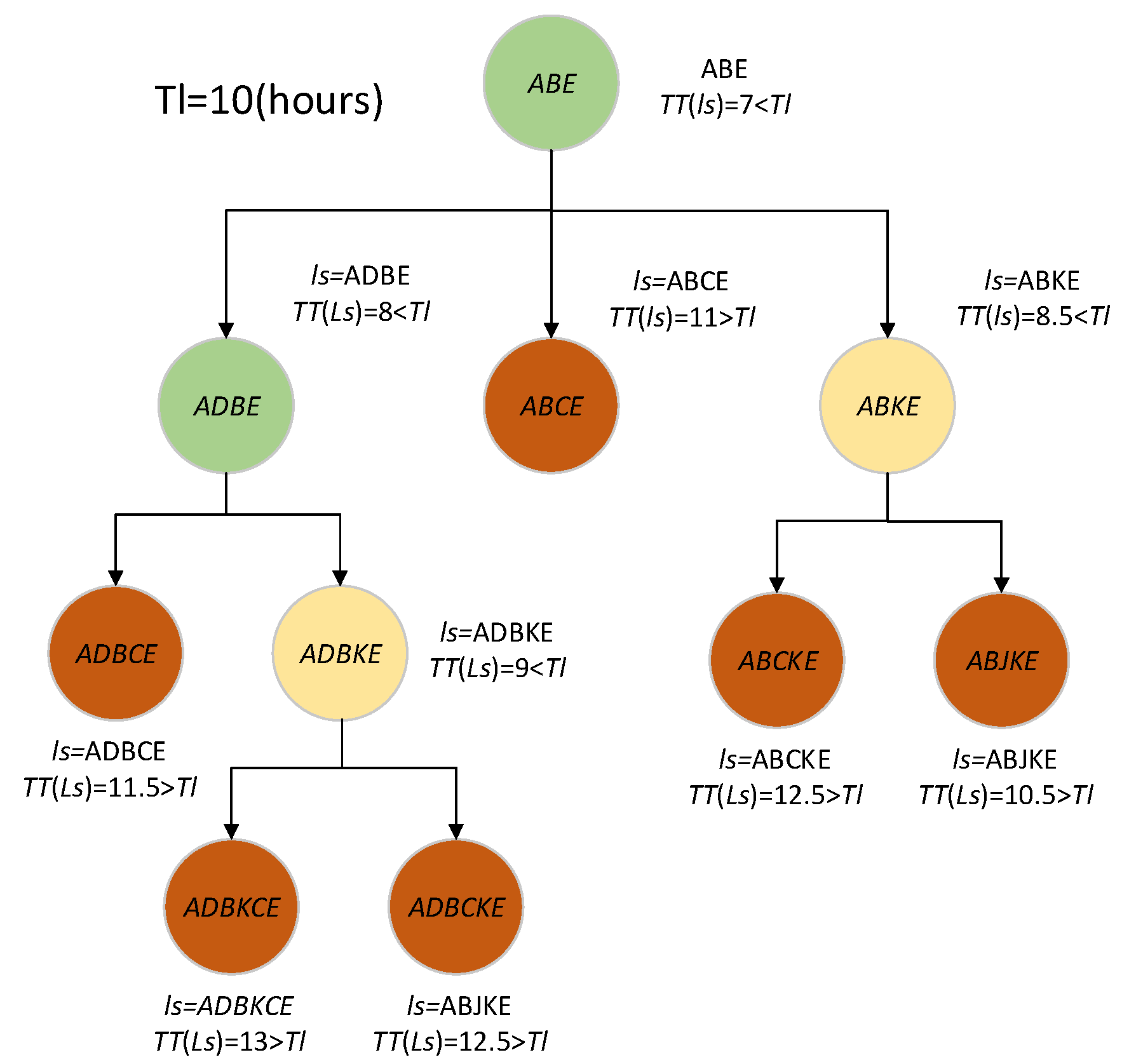
Figure 2 illustrates the process of the sequence extension function $f\left(ls,L,Tl\right)$. Assume $ls= <ABE>$, $Tl=10$ h. If $Tl\left(<ABE>\right)=7$ h, $<ABE>$ will be extended since $TT\left(<ABE>\right)<10$. Assume the sequence extension function $SeqExtention\left(<ABE>,L,10\right)$ returns $\{<\mathrm{A}\mathrm{D}\mathrm{B}\mathrm{E}>,<\mathrm{A}\mathrm{B}\mathrm{C}\mathrm{E}>,<\mathrm{A}\mathrm{B}\mathrm{K}\mathrm{E}>\}$ and $TT\left(<\mathrm{A}\mathrm{D}\mathrm{B}\mathrm{E}>\right)=8$, $TT\left(<\mathrm{A}\mathrm{B}\mathrm{C}\mathrm{E}>\right)=11$, and $TT\left(<\mathrm{A}\mathrm{B}\mathrm{K}\mathrm{E}>\right)=8.5$, respectively. Since $TT\left(<\mathrm{A}\mathrm{B}\mathrm{C}\mathrm{E}>\right)\ge 10$, $<\mathrm{A}\mathrm{B}\mathrm{C}\mathrm{E}>$ will not be extended anymore. The candidate sequences returned by $SeqExtention\left(<\mathrm{A}\mathrm{D}\mathrm{B}\mathrm{E}>,L,10\right)$ are $\{<\mathrm{A}\mathrm{D}\mathrm{B}\mathrm{C}\mathrm{E}>,<\mathrm{A}\mathrm{D}\mathrm{B}\mathrm{K}\mathrm{E}>\}$. Since $TT\left(<\mathrm{A}\mathrm{D}\mathrm{B}\mathrm{C}\mathrm{E}>\right)\ge 10$, sequence <ADBCE> will return $\left\{\right\}$. However, $TT\left(<\mathrm{A}\mathrm{D}\mathrm{B}\mathrm{K}\mathrm{E}>\right)<10$, $SeqExtention\left(<\mathrm{A}\mathrm{D}\mathrm{B}\mathrm{K}\mathrm{E}>,L,10\right)$ will return $\{<\mathrm{A}\mathrm{D}\mathrm{B}\mathrm{K}\mathrm{C}\mathrm{E}>,<\mathrm{A}\mathrm{D}\mathrm{B}\mathrm{C}\mathrm{K}\mathrm{E}>\}$. If both $TT\left(<\mathrm{A}\mathrm{D}\mathrm{B}\mathrm{K}\mathrm{C}\mathrm{E}>\right)$ and $TT(<\mathrm{A}\mathrm{D}\mathrm{B}\mathrm{C}\mathrm{K}\mathrm{E}>)$ are greater than 10, the sequence $<\mathrm{A}\mathrm{D}\mathrm{B}\mathrm{K}\mathrm{E}>$ will return itself as the candidate sequence to its parent <ADBE>. Since <ADBE> receives non-empty children’s return, which is <ADBKE>, <ADBE> will return <ADBKE> as a candidate sequence to <ABE>. A similar process will be conducted for <ABKE>. Since the traveling times of candidate sequences returned by $SeqExtention\left(<\mathrm{A}\mathrm{B}\mathrm{K}\mathrm{E}>,L,10\right)$, $\{<\mathrm{A}\mathrm{B}\mathrm{C}\mathrm{K}\mathrm{E}>,<\mathrm{A}\mathrm{B}\mathrm{J}\mathrm{K}\mathrm{E}>\}$, are all greater than 10, $<\mathrm{A}\mathrm{B}\mathrm{K}\mathrm{E}>$ will return itself as the candidate sequence. Finally, the candidate sequence $\{<ADBKE>, <ABKE>\}$ will be obtained. Note that both green and yellow nodes perform the extension process. The green node represents a better solution that can be found in its children, but the yellow node represents no better solution found in its children. The red node represents that the extension process is unnecessary since the itinerary’s traveling time exceeds the time limitation.

4. Implementation

4.1. Dataset Collection

The dataset utilized in this study was obtained through the online Flickr API. The API was used to collect the metadata information from photos taken between 1 January 2013 and 31 December 2022, within a 16 km radius of the center of San Francisco, California. The dataset includes 1,666,957 photo records contributed by 21,418 unique users. As shown in

Table 4. The example photo records.

Photo ID	Owner ID	Date Taken	Latitude	Longitude
12187393986	72350101@N03	1 January 2013 00:00	37.761027	−122.434
12186776345	72350101@N03	1 January 2013 00:01	37.800986	−122.478
8758944497	49743098@N00	1 January 2013 07:17	37.794702	−122.402
8377458549	83723104@N05	1 January 2013 08:02	37.801239	−122.425
9277954217	97871741@N07	1 January 2013 09:39	37.827946	−122.482

, each record includes the photo ID, owner ID, photo taken time, latitude, and longitude of the photo. After eliminating duplicated and incomplete records, 1,027,774 records contributed by 21,418 unique users are studied in the following implementation.

4.2. The Implementation Example

Forty-five popular attractions in San Francisco were selected from Wikipedia, Planetware, Tripadvisor, and Yelp as the set of POIs. This enables the modeling of high-frequency tourist behavior, though we acknowledge that expanding the POI set in future studies could further improve itinerary granularity and diversity. In addition, eight categories, including Active Life, Education, Food, Public Service & Government, Shopping, Arts & Entertainment, Event Planning & Service, and Others, are used to describe the characteristics of POIs.

The POI assignment process was carried out by calculating the Haversine distance between the coordinates of each check-in record and all 45 POIs. After the POI assignment, the dataset was reduced to 494,474 photo records contributed by 5945 unique users. Next, a user’s consecutive photo records at the same POI are aggregated as one visiting record. Through aggregation, the final dataset consists of 110,219 itineraries contributed by 3469 users from 156,134 visiting records. Among them, the number of itineraries with length 1 is 86,583, those with length 2 to 5 is 50,462, those with length 6 to 10 is 14,940, and those with length 10 or above is 4149. The example itineraries in the dataset are shown in

Table 5. The example itineraries.

Itinerary ID	Owner ID	POI ID	Arrival Time	Departure Time
1	100061618@N03	4	9 October 2013 16:27:00	9 October 2013 16:37:00
2	100061618@N03	18	13 October 2013 12:40:00	13 October 2013 14:16:00
2	100061618@N03	5	13 October 2013 14:22:00	13 October 2013 16:19:00
…	…	…	…	…
110219	99942665@N00	10	27 December 2017 05:31:00	27 December 2017 06:06:00
110219	99942665@N00	28	27 December 2017 07:37:00	27 December 2017 07:47:00
110219	99942665@N00	2	27 December 2017 08:08:00	27 December 2017 08:48:00
110219	99942665@N00	12	27 December 2017 10:45:00	27 December 2017 10:55:00

.

In this implementation, one day is divided into four time slots, which are ${TS}_1$ = (07:00, 13:00], ${TS}_2$ = (13:00, 18:00], ${TS}_3$ = (18:00, 22:00], ${TS}_4$ = (22:00, 07:00]. Based on Equation (1), the time preference of all users in each time slot can be derived. Similarly, the category preference of all users can be obtained using Equation (5). Finally, by combining the time and category preferences, the user preference vector for 3469 users can be obtained. For example, the preference vector for user 100061618@N03 will be <0.388889, 0.555556, 0.555556, 0.000000, 0.00980, 0.000000, …, 0.06331>, where the dimension of the vector is 12 (=4 + 8).

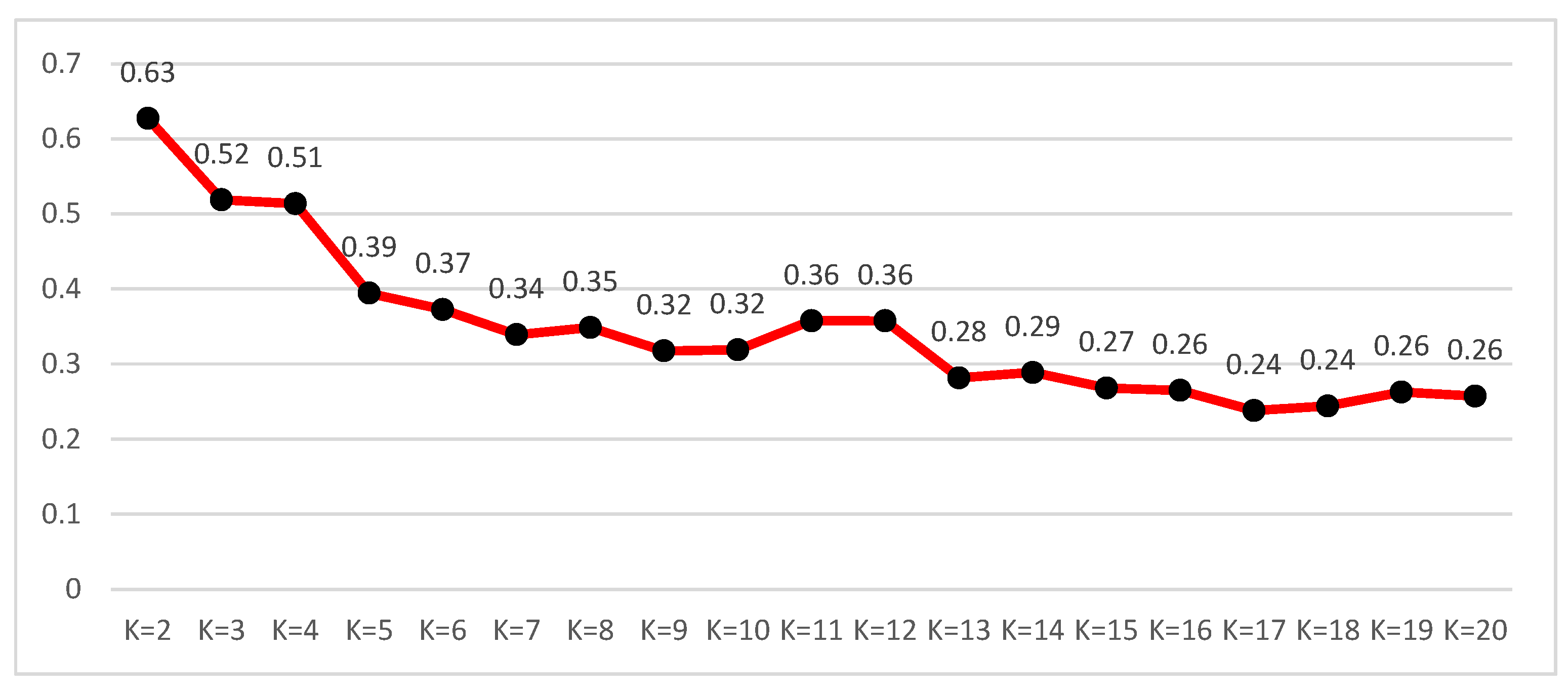
Next, the K-Means algorithm is conducted based on users’ preference vectors. We used threshold-based Haversine distance matching to reduce the likelihood of POI misclassification and filtered out ambiguous or borderline assignments. Consecutive visits to the same POI were aggregated to enhance robustness further. Figure 3 shows the silhouette values, which measure the cohesion and separation of data points within clusters when the K value is changed from 2 to 20. Based on the figure, K = 2 is selected for the following study since the silhouette value is the highest. When K = 2, the number of users in Group 1 is 1167 and that in Group 2 is 2302. In addition, 1167 users contributed 34,234 itineraries in Group 1, while 2302 users contributed 75,985 in Group 2.

Then, the sequential pattern mining algorithm is adopted to generate the frequent sequential patterns for each group. For Group 2, when the minimum support value is 5, 12,353 frequent sequential patterns are generated. Among 12,353 sequences, 45 are length 1, 1622 are length 2, 7488 are length 3, 2812 are length 4, and 386 are lengths greater than or equal to 5. The example frequent sequences are presented in

Table 6. The frequent sequential patterns for Group 2.

The Frequent Sequential Pattern Sets with Different Length	Frequent Sequential Patterns with Support Value
$L_1$	<28>: 0.0924, <9>: 0.0651, <10>: 0.0647, …
$L_2$	<10, 42>: 0.00453, <7, 8>: 0.00443, …
$L_3$	<10, 42, 13>: 0.000907, <7, 8, 10>: 0.000835, …
$L_4$	<16, 38, 35, 37>: 0.000327, <8, 10, 42, 13>: 0.000254, …
$L_5$	<7, 8, 10, 42, 13>: 0.000145, <16, 38, 35, 37, 43>: 0.000109, …
$L_6$	<13, 14, 16, 38, 35, 15>: 0.000073, <28, 7, 8, 10, 42, 13>: 0.000064, …

, where $L_1$ to $L_6$ are the set of lengths 1 to 6 frequent sequences in Group 2.

$L_1$$L_2$$L_3$$L_4$$L_5$$L_6$ For a better explanation, let us take user “37996593020@N01”, whose real-life itinerary is [30, 41, 2, 17, 10, 9] with a travel time of 8 h 28 min, as the target user. First, the group to which the target user belongs is identified. Since the similarity between the target user and the centroid of Group 1 is 0.8674 and the similarity between the target user and the centroid of Group 2 is 0.9391, the target user will belong to Group 2. Next, the input to the SPM-IR algorithm is as follows: the starting POI as POI 30, the ending POI as POI 9, the minimum time length of the candidate sequence as 8 h 28 min, the number of recommended itineraries as 5, and the set of frequent sequential patterns from Group 2. With the inputs, the SPM-IR algorithm generated 26,625 candidate sequences and returned the Top 5 recommendations, which are shown in

Table 7. Top 5 itinerary recommendations.

Candidate Sequence	POI Preference Score	Time-Matching Score	Distance Score	Itinerary Score	Ranking
[30, 13, 42, 8, 7, 6, 8, 10, 9]	0.981664	0.643959	0.182501	0.814374	1
[30, 13, 16, 37, 43, 8, 10, 9]	0.67047	0.880845	0.152377	0.799646	2
[30, 13, 12, 44, 42, 10, 8, 7, 9]	0.803416	0.723712	0.128304	0.799608	3
[30, 13, 12, 44, 42, 10, 7, 8, 9]	0.803416	0.723712	0.128433	0.799565	4
[30, 13, 42, 7, 6, 7, 8, 10, 9]	0.926526	0.638737	0.181342	0.794640	5

.

4.3. Comparisons

Similar to the case in Section 4.2, itineraries with at least five lengths in Group 2 are used as the dataset for comparison. Therefore, 500 itineraries that generate 2190 frequent sequential patterns by the sequential pattern mining algorithm are used as the real-life test dataset.

4.3.1. Evaluation Metrics

For each real-life itinerary $I$ in the testing set, we can derive its starting POI, ending POI, and itinerary time and input to the SPM-IR algorithm to generate a set of candidate sequences ${\widehat{I}\in L}_{candidate}$. The score of the real-life itinerary (i.e., $\mathrm{S}\mathrm{c}\mathrm{o}\mathrm{r}\mathrm{e}\left(I\right)$) and the score of a candidate sequence (i.e., $\mathrm{S}\mathrm{c}\mathrm{o}\mathrm{r}\mathrm{e}(\widehat{I}$)) can be evaluated using Equation (18). To assess the performance of different methods, the following metric is employed in this study:

Outperformance Rate (OR): OR counts the number of candidate sequences whose itinerary score exceeds the real-life itinerary’s score, divided by the total number of candidate sequences. A higher value indicates that the method produces superior itineraries than the real-life one. The definition of OR is as follows:

$$OR={\displaystyle \frac{{\sum }_{\widehat{I}\in L_{candidate}}\delta (Score\left({\widehat{I}}_u\right)>Score\left(I_u\right))}{‖L_{candidate}‖}}$$

(19)

where $\delta \left(·\right)=1$ if the condition is true; otherwise, $\delta \left(·\right)=1$.

Let us take the real-life itinerary [30, 41, 2, 17, 10, 9] described in Section 4.2 as an example. As shown in

Table 8. The score details and ranking for the real-life itinerary.

Real-Life Itinerary	POI Preference Score	Time-Matching Score	Distance Score	Itinerary Score	Ranking
[30, 41, 2, 17, 10, 9]	0.190663	0.239972	0.454386	0.325416	25,246

, the itinerary score of the real-life itinerary is 0.32542 and is ranked 25,246 among 26,625 candidate sequences generated by the SPM-IR algorithm. Therefore, the percentage that generated candidate sequences are better than itinerary l is OR = 25,246/26,625 = 94.82%. That is, 94.82% of the generated candidate sequences are better than [30, 41, 2, 17, 10, 9] regarding the itinerary score.

4.3.2. Ablation Study for User Preference

User preference is important to a personalized sequence recommendation system. This is especially true in our system since user preferences are used to identify similar user groups for later recommendations. This research integrates time preference (TP) and category preference (CP) as the final user preference. In this section, we conducted an ablation study to verify the validity of the two components in the final recommendation. The ablation experiments consist of three parts:

▪

-TP: to verify the performance of the category preference, we removed the time preference.

▪

-CP: to verify the performance of the time preference, we removed the category preference.

▪

Full: consider both TP and CP in this study.

Figure 4 shows the results of the ablation experiment. The experimental results indicate that the best OR metric (46.181%) occurred when TP and CP were considered (e.g., Full). The improvement was 5.9% compared to CP only and 8.23% in OR compared to TP only. In addition, adopting category preference (-TP) achieves a better OR metric (43.609%) than adopting time preference only (-CP) (42.364%).

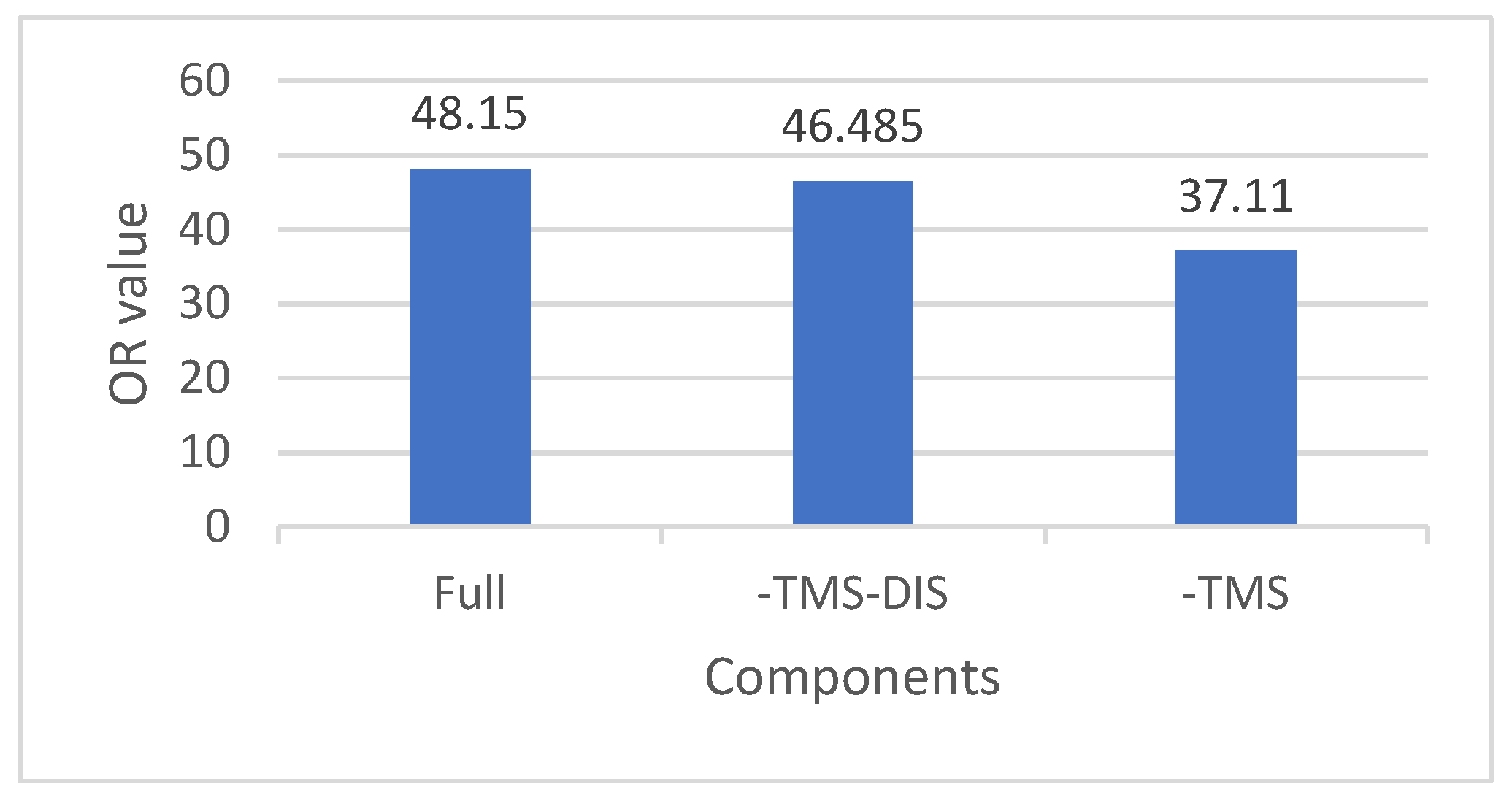
4.3.3. Ablation Study for Itinerary Score

The itinerary score is important to evaluate the suitability of an itinerary in our system. This research integrates the POI preference score (PPS), time-matching score (TMS), and itinerary distance score (DIS) as the itinerary score to make a better itinerary evaluation. We conducted the following ablation experiment to verify the validity of the three components in the final recommendation. The ablation experiment consists of three parts:

▪

-TMS: to verify the performance of PPS and DIS, we removed TMS.

▪

-TMS-DIS: to verify the performance of PPS, we removed TMS and DIS.

▪

Full: considers PPS, TMS, and DIS simultaneously.

Figure 5 shows the results of the ablation experiment. The experimental results indicate that the best OR metric (48.150%) occurred when PPS, TMS, and DIS are considered in the itinerary score (e.g., Full). Removing TMS gives the most significant deduction (11.04%) in the OR metric. This shows that TMS is the most important component in the itinerary score design.

5. Conclusions

In this paper, we presented a novel personalized itinerary recommendation system that addresses key limitations in the existing approaches. Our system first clusters users with similar temporal and categorical preferences, enabling more targeted sequential pattern mining for each group. We then introduced a comprehensive itinerary evaluation incorporating three critical dimensions: POI preference score, time-matching score, and travel distance score. This approach ensures that the recommendation results align with user interests, optimizing visit timing and travel efficiency. Finally, our Sequential-Pattern-Mining-based Itinerary Recommendation (SPM-IR) algorithm extends beyond feasible solutions to near-optimal ones by systematically checking and extending frequent sequential patterns within user-specified constraints. The system returns top-N ranked itineraries that balance personal preferences with practical travel considerations, providing a more holistic approach to personalized travel planning.

A real-life dataset from geotagged social media is implemented to demonstrate the benefits of the proposed personalized itinerary recommendation system. Using a real-world dataset of over 494,000 POI-tagged photos and 110,219 itineraries from 3469 users, the system successfully clustered users and generated 12,353 frequent sequence patterns. For the evaluated target itinerary, 94.82% of the generated candidate sequences achieved a higher itinerary score than the real-life sequence. Moreover, ablation studies showed that incorporating both time and category preferences improved performance by up to 8.23% and that the time-matching score was the most critical component, contributing an 11.04% boost in itinerary quality. These results validate the effectiveness of the proposed multidimensional user profiling and itinerary-scoring approach.

Despite the promising results of the proposed SPM-IR system, several limitations should be acknowledged. First, while the Flickr dataset offers rich spatiotemporal travel records, we acknowledge that its users may not fully represent the general tourist population. Therefore, findings should be interpreted cautiously, and future work should validate the model with more diverse datasets. Second, we used threshold-based Haversine distance matching to reduce the likelihood of POI misclassification and filtered out ambiguous or borderline assignments. Consecutive visits to the same POI were aggregated to enhance robustness further. Future improvements could incorporate semantic or image-based verification of visited sites. Third, while the proposed itinerary score incorporates POI preference, time matching, and travel distance, other influential factors such as transportation mode, weather conditions, or budget constraints were not considered. Fourth, the sequence extension process is based on existing frequent patterns, which may limit its ability to generate highly novel routes for users with unique interests. These limitations allow future research to incorporate more contextual variables, expand data sources beyond social media, and enhance adaptability for niche user groups. Nonetheless, this study provides important implications for designing intelligent travel recommendation systems, emphasizing the value of integrating user segmentation, multi-criteria evaluation, and flexible sequence expansion to deliver more personalized and practical travel itineraries.

Several possible extensions and improvements can be considered for future research. First, the dataset used in this study is based on the Flickr dataset of San Francisco, California. However, the selection method of specific POIs can impact the performance of the proposed method. Further investigation can explore methods to determine the optimal number of POIs and refine the selection process. Second, sequential pattern mining heavily relies on the user experience and may encounter data sparsity issues with insufficient visiting records. Collecting more user data can significantly improve the performance of the proposed method. Third, it would be beneficial to conduct comparative studies with other existing methods using the pairwise comparisons method [35] to understand the system’s effectiveness and performance better. Finally, due to data limitations, the current model does not incorporate contextual factors such as weather, local events, or travel group size. Future research could enhance the model’s realism and precision by integrating such variables from complementary data sources (e.g., event APIs, weather data, or survey input).