Article

Power Profiling of Smart Grid Users Using Dynamic Time Warping †

by
Minchang Kim
1,2,
Mahdi Daghmehchi Firoozjaei
3,
Hyoungshick Kim
1,* and
Mohamad El-Hajj
3
1
Department of Electronical and Computer Engineering, Sungkyunkwan University, Suwon 16419, Republic of Korea
2
Satellite Communication Research Devision, Electronics and Telecommunication Research Institute (ETRI), Daejeon 34129, Republic of Korea
3
Department of Computer Science, MacEwan University, Edmonton, AB T5J 4S2, Canada
*
Author to whom correspondence should be addressed.
This article is a revised and expanded version of a paper entitled Time-Series Load Data Analysis for User Power Profiling, which was presented at the ICACT 2023 Conference, Kyunggi-do, Republic of Korea, 19–22 February 2023.
Electronics 2025, 14(10), 2015; https://doi.org/10.3390/electronics14102015
Submission received: 13 February 2025 / Revised: 28 March 2025 / Accepted: 9 May 2025 / Published: 15 May 2025

Abstract

:
Power consumption data play a crucial role in demand management and abnormality detection in smart grids. Despite its management benefits, analyzing power consumption data leads to profiling consumers and opens privacy issues. To demonstrate this, we present a power profiling model for smart grid consumers based on real-time load data acquired from smart meters. It profiles consumers’ power consumption behavior by applying the daily load factor and the dynamic time warping (DTW) clustering algorithm. Due to the invariability of signal warping of this algorithm, time-disordered load data can be profiled and consumption features can be extracted. By this model, two load types are defined and the related load patterns are extracted for classifying consumption behavior by DTW. The classification methodology is discussed in detail. To evaluate the performance of the proposed model for profiling, we analyze the time-series load data measured by a smart meter in a real case. The results demonstrate the effectiveness of the proposed profiling method, achieving an F-score of 0.8372 for load type clustering in the best case and an overall accuracy of 77.17 % for power profiling.

1. Introduction

With the advent of smart meters and their advanced features, load data can now be analyzed more quickly and accurately in the smart grid. Advanced metering infrastructure (AMI), as a core technology, provides bidirectional information flow between utility providers and consumers. It accesses each individual location in real time and uploads a vast amount of data to the smart grid [1,2]. These data allow for improved management of utility assets as well as demand response (DR) systems [3]. Furthermore, it reveals valuable data for profiling consumers’ power consumption and analyzing their usage behavior [4].
Power consumption is a critical variable for expansion planning, load forecasting, performance analysis, and demand management in smart grids [5,6,7]. Analyzing consumers’ power consumption behavior, known as power profiling, is essential for demand forecasting and optimizing resource allocation. The power profile of a consumer reveals their power consumption patterns over a specific period and serves as a valuable tool for various smart grid applications, such as DR and load forecasting [8,9]. Various methods have been employed to extract and classify patterns for power profiling, often relying on representative data and statistical averages of electrical appliance usage [10].
In reality, a power profile is influenced not only by the load patterns of electrical appliances but also by consumers’ consumption behavior and contextual factors such as time, location, and environment [10,11,12,13]. Given these factors, comprehensive power profiling is categorized into three concepts: user, device, and context [14]. The overall power profile results from a combination of these concepts. Accurate resources and analytical methods are crucial for determining load curve characteristics and identifying consumer power consumption behavior. Although more realistic power profiles lead to more accurate demand management, collecting fine-grained metering measurements provides additional information about consumers’ daily life patterns [15,16]. This potentially raises privacy concerns for consumers, particularly with regard to untrusted third parties.
In this paper, we introduce a model to analyze consumers’ power consumption, describe their power usage behavior, profile their power usage, and predict consumption based on these profiles. It analyzes consumers’ consumption behaviors in a realistic environment affected by the time factor. To build a time-invariant consumer-level load clustering, we perform load data time-series correlation using the dynamic time warping (DTW) algorithm [17]. DTW is selected to measure the similarity between the power usage time-series due to its properties, namely, signal warping invariability and implementation simplicity. By clustering the consumers’ load data with the DTW algorithm, load forecasting is performed by correlating the historical load data and time-series of the new power usage data. We use the electricity consumption data extracted from the Almanac of Minutely Power Dataset Version 2 (AMPds2), available at Harvard Dataverse [18]. The AMPds2 is a real-world dataset that captures all three main types of consumption, including electricity, water, and natural gas, collected from a house in the Greater Vancouver metropolitan area, Canada, over a long period of time (two years) [18]. Short-term power usage data acquired by real-time smart meters are used to extract load patterns and generate realistic power profiling. The similarities between the short-term electricity consumption data points measured by DTW are used to extract the consumers’ load patterns. Furthermore, the variations and patterns in the daily load factor [19] are examined to understand and analyze users’ consumption behavior.
The main contributions of this paper are as follows:
Extracting power consumption patterns by measuring the DTW similarity between a consumer’s load data time series.
Power profiling based on the signal warping invariability property of the DTW algorithm. Thus time-disordered load data can be used for detecting consumption patterns and load type clustering.
Enhancing user power profiling by including daily load factor analysis and monitoring user’s consumption behavior, device’s power usage patterns, and the context.
The remainder of this paper is structured as follows: Section 2 reviews related work, while Section 3 describes the research methodology. Section 4 outlines the preliminaries of our model. In Section 5, we present our proposed model, detailing its stages, including power load data extraction, analysis, clustering, and profiling, and we evaluate the accuracy of our power profiling approach. Section 6 discusses potential privacy concerns associated with power profiling. Finally, Section 8 concludes the paper and outlines directions for future research.

2. Related Work

User consumption data are analyzed for various purposes, including modeling energy consumption trends, anomaly detection [20], predictive modeling, and visualization. In this section, we provide an overview of existing research in power consumption forecasting, anomaly detection, and user profiling as they relate to our work. Time-series analysis techniques are widely used to model and forecast energy consumption trends [21]. For instance, in [22], regression models were developed using load data time series to predict consumption. C. Li proposed a short-term load forecasting method to extract load patterns from consumption data [23]. Clustering consumption time series is commonly employed to monitor power consumption in smart grid applications for purposes such as demand forecasting and anomaly detection. Son et al. [24] applied forecasting models to predict electricity demand for industrial consumers using time-series clustering. Maurya et al. [25] introduced an enhanced version of the D-Stream clustering algorithm to monitor power demands in smart grids. The resulting clusters were used to detect abnormalities in users’ consumption, such as defective appliances. Additionally, in [26], smart grid users were classified by clustering their consumption data obtained from smart meters, and this classification was leveraged to forecast power consumption.
Measuring the distance between power consumption time series has been widely used to detect anomalies in operation or malicious activities, such as energy theft [27,28,29,30,31,32]. Tao et al. [27] identified anomalies in smart meter devices by analyzing correlation patterns in power consumption data. A combination of DTW and k-nearest neighbors (KNN) was employed in [28] to detect malicious activities such as data tampering and manipulation. In this work, DTW measured the similarity between usage time series, while KNN ranked anomalous behavior. Villar-Rodriguez et al. [29] detected users’ behavioral changes by measuring the DTW distance in usage data, identifying anomalies caused by malfunctions or fraudulent activities. Similarly, Hassan et al. [30] used a combination of a convolutional neural network (CNN) and a long short-term memory (LSTM) model to detect electricity theft by analyzing power consumption time series. In [31], the authors introduced a photovoltaic power prediction model based on FastDTW, which is a computationally efficient approximation of DTW with linear time and space complexity [32]. This model predicted users’ power consumption by identifying consumption similarities over different time durations.
Profiling users in smart grids has been studied for various purposes, such as optimizing energy usage, detecting anomalies, and providing personalized services [33,34,35]. In [34], Cheung et al. proposed a clustering model to profile smart grid consumers with or without solar panels (e.g., rooftop photovoltaic (PV) systems) for demand prediction. This load profiling allowed for the distinction of PV users and facilitated their inclusion in dedicated demand response programs. The results also provided insights into the relationship between socio-demographic factors and PV installations. Jindal et al. [35] discussed two data-driven schemes, at the smart meter level and at an aggregate level, to profile users’ consumption and detect potential power theft. Liu et al. [36] proposed an electric vehicle (EV) charging schedule algorithm aimed at minimizing power fluctuations. EV users were profiled based on their power loading behavior, such as connection times, battery residuals, and expected state-of-charge levels. Smart grid user profiling was further explored in [37] to monitor individuals suffering from self-limiting conditions (e.g., Alzheimer’s, Parkinson’s disease, and clinical depression). Changes in a consumer’s power usage behavior were used to assess their well-being or state of mind.

3. Research Methodology

The primary objective of this study is to develop a profiling model that analyzes power consumption data to extract users’ behavioral insights in the smart grid. The key challenges include the limited scope of the dataset used in this work, as it contains data from only a single household. Additionally, the use of DTW for pattern analysis introduces computational constraints. Another challenge is balancing data utility with privacy preservation in user profiling.

3.1. Research Approach

This study follows a data-driven approach, leveraging power consumption data from the AMPds2 dataset. The methodology consists of the following steps:
Data collection and preprocessing: extracting appliance-level power consumption data from AMPds2.
Feature extraction and profiling: using DTW to analyze consumption patterns and generate behavioral profiles.
Evaluation and comparison: assessing the effectiveness of the model.

3.2. Tools and Techniques

The following tools and techniques are used:
Dataset: AMPds2 dataset (detailed in Section 5.1).
Algorithm: DTW for sequence comparison.
Implementation: Python programming with DTW library.
Computational Environment: The implementation was conducted using Python 3.11 64-bit in a standard computing environment, with details provided in Section 5.2.

4. Preliminaries and Background

4.1. Time-Series Classification

Time-series classification has many applications in industry and the energy market. Classification methods can be either feature-based or distance-based. In feature-based methods, a statistical [38] or symbolic [39] feature representation is defined for the time series and machine learning methods are used. In distance-based methods, the similarity between two time series is computed by a predefined distance function. Euclidean distance (ED) [40], KNN [41], and DTW [42] are some of the most commonly used distance functions [43].

4.1.1. Euclidean Distance (ED)

The ED algorithm is the most common similarity metric. It is appropriate for applications where there is no direct correlation among distinct features [44]. The ED algorithm uses the straight-line distance between two points. Given two time series P = ( p 1 , p 2 , , p n ) and Q = ( q 1 , q 2 , , q n ) in n dimensions, the E D between them is
E D ( P , Q ) = i = 1 n ( p i q i ) 2 ,
where p i and q i are the coordinates of P and Q in dimension i. Due to its simplicity, efficiency, and status as a distance metric, E D is a popular distance measure for many data mining tasks. However, it is only applicable to equal-length series with equal dimensions and is very sensitive to mismatches between the series. For example, if there is a slight delay or time shift in one of two otherwise identical time series, the ED between them will be unreasonably large [43]. This sensitivity leads to inaccuracies in classification and clustering applications, despite its ease of implementation and time efficiency [45].

4.1.2. k-Nearest Neighbor (KNN)

The KNN is a classification method used in machine learning. It is a suitable choice for classification when there is little or no prior knowledge about the data distribution [46]. In this classification method, the k-nearest neighbors are used to determine the class. Based on the similarity between the new data and the available data points, the new data are classified in the most similar category. Similarity is defined according to a distance metric (e.g., ED) between two data points. For each new data point, a positive integer k is specified, and the k entries in the database closest to the new data are selected [47]. Assume x is a sample, where C is the true class, and C p is the predicted class for this test sample, where C , C p = 1 , 2 , , M . Here, M is the total number of classes. In 1-nearest neighbor classification, the predicted class of sample x is set equal to the true class C of its nearest neighbor, where m i is a nearest neighbor to x if it has the minimum distance [46]:
d ( m i , x ) = m i n j [ d ( m j , x ) ] .
For k-nearest neighbors, the predicted class of the test sample x is set equal to the most frequent true class among k nearest training samples. This forms the decision rule [46]:
D : x C p .
The sensitivity of k is a key issue in KNN classification and can degrade its performance (e.g., high error formation) [48,49,50]. Selecting the proper number of neighbors for clustering is crucial. An optimal number of neighbors should be considered for classifying new data [48].

4.1.3. Dynamic Time Warping (DTW)

Compared to ED, DTW is more robust in similarity computation. DTW is a very popular tool in temporal data mining, and its distance comparison is less sensitive to signal transformations such as shifting, uniform amplitude scaling, or uniform time scaling [51]. DTW-based time-series similarity measures are less affected by time distortion. It allows elastic transformation of time series to detect similar shapes with different phases. Since DTW is invariant to signal warping, such as scaling in the time axis or the Doppler effect, it is preferred for pattern matching tasks [52].
To find the distance between two time series X = ( x 1 , , x i , , x n ) of length n and Y = ( y 1 , , y j , , y m ) of length m, DTW is computed by first finding the best alignment between them. An n-by-m matrix is constructed, in which its (ith, jth) element is equal to ( x i y j ) 2 , representing the cost to align the point x i of time series X with point y j of time series Y. An alignment between the two time series is represented by a warping path, W = w 1 , w 2 , , w K , in the matrix. The path must be contiguous, monotonic, start from the bottom-left corner, and end at the top-right corner of the matrix. The warping path has a length K, which is
m a x ( n , m ) K < ( | n | + | m | ) .
The kth element of the warping path, W, is w k = ( i , j ) , where i and j are corresponding indices from time series X and Y, respectively [32]. The best alignment is given by a warping path through the matrix that minimizes the total cost of aligning its points. The minimum total cost is the D T W distance, as follows [43,53]:
D T W ( X , Y ) = a r g m i n ( W ) = k = 1 , w k = ( i , j ) K ( x i y i ) 2 .
To compute the minimum cost alignment, dynamic programming (DP) is used, which increases the complexity of the computation. More critically, DP is a sequential process, making DTW non-parallelizable. Some techniques have been proposed to parallelize DP [52].

4.2. Daily Load Factor

To measure the utilization rate and indicate consumers’ usage behavior, load factor is defined as an expression of how much energy was actually used compared to the peak demand. A daily load factor ( d l f ) is defined as the ratio of daily power mean to daily maximum power demand [19], as follows:
d l f = ( 1 m k = 1 m 1 / n i = 1 n P i m a x ( P i , 1 i n ) ) × 100 ,
where P i is the electrical usage in W, which is periodically measured (e.g., measured of each 10 min period), n is the number of power data points in a day, and m is the total number of days. A larger d l f corresponds to a load type in which more electricity is consumed evenly across the day, whereas a low d l f indicates small intervals of high electricity consumption. In fact, a larger factor shows a smoother power consumption pattern across the day and efficient electricity management [19,54]. Load factors vary depending on consumer’s behavior, a device’s power consumption patterns, and the context, e.g., weather and usage frequency.
Generally, consumers’ power demand curves are optimized by increasing their minimum load consumption and/or decreasing their maximum load consumption. To this end, load factor values are analyzed to evaluate and optimize the power demand curves. Optimizing the load factor (equal to 1) by minimizing the differences between the maximum and the average power demand leads to an optimum power demand curve [55].

4.3. Performance Metrics

To evaluate the classification performance, a confusion matrix [56] is used. The confusion matrix, also known as the error matrix, is a table that describes the performance of a classification model on a set of test data where the true values are known [57]. As shown in Table 1, it is a two-dimension matrix, one dimension represents the actual class of an object, and the other represents the class predicted by the classifier [58]. The confusion matrix represents four values, namely true positive (TP), false positive (FP), true negative (TN), and false negative (FN). TP values are correctly classified, FP values are wrongly classified into the relevant class, FN values belong to another class when they should be in the relevant class, and TN values are correctly classified values in the other class [59].
Based on confusion matrix values, several metrics are defined to evaluate classification performance. The most commonly used performance metrics are accuracy ( A C C ), precision (P), sensitivity ( S n ), specificity ( S p ), and F-score values [56,59]:
Accuracy indicates the proportion of correct predictions, reflecting the true positive rate:
A C C = ( T P + T N ) T P + F P + T N + F N .
Precision shows the positive predictive value:
P = T P T P + F P .
Sensitivity, or recall, shows the true positive rate, indicating the rate of correctly labeling objects of a certain class. For a good classifier, it should ideally be 1 (high) and is calculated as follows:
S n = T P T P + F N .
Specificity, or the true negative rate, indicates the rate at which negative objects are correctly labeled. For a good classifier, it should ideally be 1 (high) and is calculated as follows:
S p = T N T N + F P .
The F s c o r e is a way to measure a classification model’s accuracy and is the harmonic mean of recall and precision, as follows:
F s c o r e = 2 × ( P × S n ) P + S n .
In classification, the higher the F s c o r e , the more accurate the model is. The highest value of the F s c o r e is 1.0 , which indicates perfect precision and recall. The lowest possible value is 0, which occurs if either precision or recall is zero.

4.4. Power Profiling

Power profiling includes analytical approaches that lead to predictive maintenance, abnormality detection, and fault detection. While most consumers show variable power consumption behavior, they typically exhibit a certain amount of repetitiveness [5,60]. Consumers’ consumption behavior is affected by their social, professional, and economic situations, the appliances they use, the time of day, and environmental factors such as weather and dwelling conditions. These factors can be considered random or complex phenomena [61].
Power profiling is also used to predict and balance electricity purchases and sales. Poor estimation can be costly for a utility provider [62]. Personalizing power management and understanding electrical usage patterns help utilities send proper demand signals to the DR systems to balance the electrical load. Typically, consumers are clustered based on their load curves. Consumers in the same cluster have similar consumption patterns. By recognizing the load patterns of a new consumer, they can be classified into a particular consumer group, where similar rules are applied. Furthermore, abnormal usage can be detected for this new consumer with minimal information based on the load curves of their class [9]. Beyond load prediction and abnormal usage detection, analyzing a user’s power consumption data for profiling may also lead to determining the working cycle of each residential electrical appliance [12].
Processing DR data makes it possible to determine the patterns of individual electrical loads (e.g., operating schedules). Therefore, patterns of normal and abnormal operation are available for utility engineers [60]. These patterns are used in decision tree-based schemes for fault detection or security management [63]. For instance, an abnormal increase in usage at an unusual time (e.g., during midnight or vacation time) can indicate an energy theft attack or an operational fault and should be treated accordingly.
For load management, data processing usually occurs locally in DR systems, including AMI and Non-Intrusive Load Monitoring (NILM) systems. NILM is a fundamental tool for extrapolating in-home activity. It disaggregates a consumption data stream into individual load signatures and matches them with reference signatures stored in a database to distinguish operating appliances such as refrigerators, air conditioners, and water heaters. NILM can identify specific electric device/appliance brands and might even identify malfunctioning appliances [64]. Therefore, power profiling can easily compromise consumer security and privacy. Credential extraction by power analysis attacks, authentication compromise by replay attacks and masquerading, and privacy breaches are potential security issues associated with power profiling [65].

5. Power Profiling Model

For power profiling, the consumer’s load data provided by smart meters are used to extract the required features. In this model, the profiling process is divided into four stages, namely data extraction, load data analysis, load data clustering, and power profile assignment. Power consumption is profiled by comparing the time series of the consumer’s load data, observing consumption patterns in the short term (one day), and analyzing the load factor in the long term. In this section, we explain each stage of this model in more detail.

5.1. Data Extraction

Electrical usage data in DR systems, acquired from smart meters, is used to extract consumption patterns. We use a real-world dataset of electrical consumption, AMPds2 [18], which includes load data from various electrical appliances (e.g., refrigerator, dryer, stove, and lights) collected over an extended period. The dataset was collected using DENT real-time smart meters, which track short-term power consumption and provide granular insights into daily energy usage patterns. In AMPds2, DENT PowerScout 18 units [66] were installed at the electrical circuit breaker panel to monitor appliance loads, recording data at one-minute intervals. These smart meters capture kWh/kW energy and demand data, enabling diagnostics and monitoring within a smart grid neighborhood area network (NAN) [66]. Each smart meter generates 1440 measurement data points per appliance per day. To balance computational efficiency and pattern extraction fidelity, we downsample the dataset by selecting 10-min interval readings, resulting in 144 data points per appliance per day. This time-series representation allows for efficient pattern recognition and similarity analysis using DTW. The extracted daily power usage time series serves as the basis for profiling and clustering consumption behaviors across different days.

5.2. Load Data Analysis

Power consumption patterns are extracted by measuring the similarity between daily load time series using DTW-based clustering. We implement DTW using the dtw-python package (PyPI package 1.5.3) [67] in Python due to its efficiency and robust handling of time distortions. The implementation was executed on a Windows 11 machine (following the official documentation available at https://dynamictimewarping.github.io/python/, accessed on 5 August 2024). DTW is preferred for its ability to accommodate temporal variations in energy consumption (e.g., shifts in peak usage hours) while maintaining accurate pattern alignment. In our implementation, DTW employs the following:
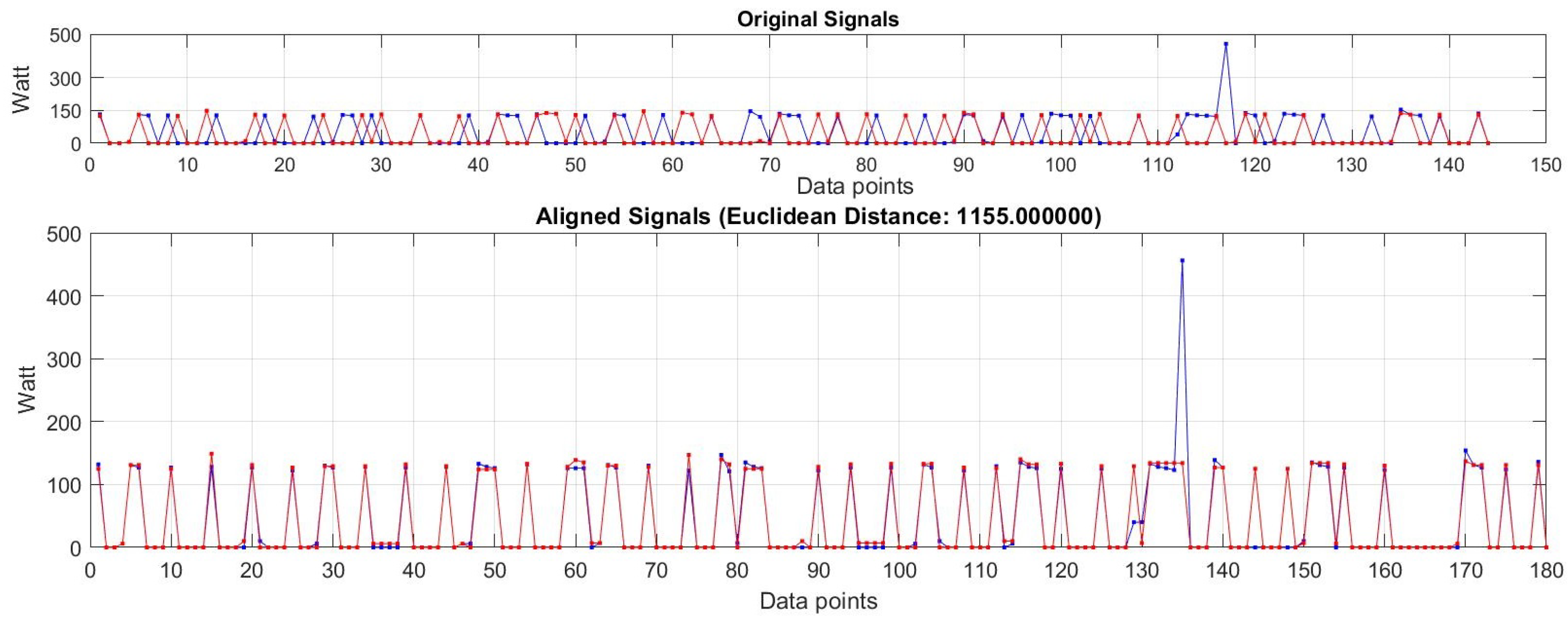
Symmetric Point-to-Point (P2P) matching, ensuring temporal consistency between aligned pairs [68].
A local continuity constraint, which allows for flexible time warping while preserving signal integrity [67].
Empirical clustering thresholds, determined through experimentation to optimize classification accuracy and robustness against outliers.
Figure 1 illustrates the DTW alignment process, where two load time series (each containing 144 data points) are compared. The DTW algorithm dynamically aligns the signals by minimizing the cumulative distance between corresponding data points, allowing for elastic matching despite fluctuations in energy usage timing.
Although the ED metric is simple to implement, we could not select it for our classification model due to its sensitivity to phase shifts and misalignment between time series. ED is primarily sensitive to amplitude similarities, meaning that even slight temporal misalignment (e.g., time distortions) can significantly increase the calculated distance, leading to misleading similarity assessments [69]. Power consumption data often fluctuate due to user habits, environmental factors, or operational changes. Even when two time series exhibit similar patterns, small temporal shifts can cause a disproportionate increase in ED. Furthermore, ED requires time series to be of equal length, which poses a limitation when comparing time series of varying lengths.
For example, Figure 2 illustrates two load data time series of different lengths. These time series represent load data from two separate days extracted from our dataset, AMPds2. Due to a technical issue (e.g., a communication error), some load measurement data are missing, resulting in fewer data points in the second time series (represented by the dotted curve). As a result, calculating the ED between these two time series produced a value error. In contrast, calculating the DTW distance between the same time series did not present any issues. By leveraging DTW’s capability to adapt to temporal variations, our model achieves more reliable clustering and profiling of power consumption behaviors, leading to improved accuracy in power profiling.

5.3. Load Data Clustering

Power consumption patterns depend on the consumer’s usage behavior, power consumption characteristics of the employed devices, and contextual factors. Consumers use power differently depending on the time of day and day of the week (weekday versus weekend/holiday). For instance, the load factor of a refrigerator is influenced by its consumption patterns, which depend on factors such as thermal load, number of door openings, and opening duration [70]. Compared to a workday, the refrigerator shows different consumption patterns on a weekend/holiday when the number of people at home is different and their behaviors vary (e.g., different sleeping times and more TV watching). Figure 3 depicts the refrigerator’s hourly electricity consumption on a workday, a weekend, and over a week, measured every 10 min. Based on this, while the refrigerator’s power consumption changes smoothly on a workday, it behaves differently during weekend hours. Typically, a refrigerator exhibits a cyclic pattern of power consumption due to the duty cycling of its compressor and operates at certain intervals during the day [12]. Figure 4 shows the pattern of power usage data for the refrigerator extracted from the AMPds2 dataset. Since the refrigerator operates continuously, its power consumption pattern can be used to profile the user’s power usage and identify unusual events. Based on these properties, we select the refrigerator as the source for profiling and evaluate its power consumption to monitor the consumer’s power behavior.
As per our power load feature, we consider two sets of power load patterns, namely workday and weekend/holiday load patterns sets. Although these sets of power load patterns can be extended to more categories (e.g., morning or afternoon, day-time or night-time, etc.), we introduce our profiling model based on these two pattern sets and develop it by adding more categories in the next phase. This binary classification serves as a foundational step for testing DTW-based clustering and evaluating its ability to distinguish meaningful load patterns. Additionally, workday and weekend consumption patterns exhibit statistically significant differences, making them a practical starting point for initial load profiling in smart grids. In this regard, we use the refrigerator’s power data points over five months (from September 2013 to January 2014) to extract the consumption features, train the model, and classify the consumer’s power load. We employ the DTW algorithm to measure the similarity between the power usage time series of those days (a total of 22,032 data samples) and set a DTW distance matrix. This matrix shows pairwise DTW distances between power usage data points on different days. To indicate the consumer’s usage behavior, we redefine the load factor for a shorter duration, an hour, as the hourly load factor. Based on the daily load factor introduced in Section 4, an hourly load factor ( l f h ) is defined as follows:
l f h = ( 1 24 k = 1 24 1 / n i = 1 6 P i m a x ( P i , 1 i 6 ) ) × 100 ,
where P i is the electrical usage in W measured of each 10 min period, in total, six power data points in an hour. The hourly load factor is the average of the ratio of hourly power mean to hourly maximum demand per day (among 24 h).
To profile power usage, we define criteria based on the DTW matrix of daily usage time series and hourly load factors. Two load profiles are defined: the workday load profile (WoLP) and the weekend/holiday load profile (WeLP). Each load type is assigned a set of criteria, including a pattern set of the power usage time series, which represents the corresponding profile (workday or weekend) and a daily load factor. To determine the pattern set for each load type, we find a daily load time series among all sample days’ load time series that has the minimum DTW distance to other similar days’ load time series during the training phase. The average DTW distance to this representative time series is a criterion used in our power profiling model. For each load type, the selected day’s load usage data time series is considered the load pattern. The second parameter used to identify the load profile is the hourly load factor, which is calculated based on Formula (12). Using these profiling criteria, a consumer’s power consumption behavior is categorized into one of two types: a workday power profile or a weekend/holiday power profile.
In Table 2, the characteristics of power load patterns sets, including DTW distance (average and standard deviation), power usage (peak and mean), and hourly load factor, are listed for both load profiles, WoLP and WeLP. In WoLP, the representative load pattern set has an average DTW distance of 1165.80 to other workdays’ load data time series. The load pattern set in WeLP has an average DTW distance of 1244.75 to other weekends’/holidays’ load data time series. As shown at this table, hourly load factors are 22.71 % and 21.35 % for workdays and weekends/holidays load types, respectively. It is noted that the workday load type has a higher hourly load factor, which indicates smoother power usage for this load type.

5.4. Power Profile Assignment

The power profile assignment stage assesses the input power usage data and clusters it into a particular power load type. It measures the similarity between the input load data time series with both load patterns sets of WoLP and WeLP using the DTW algorithm. Depending on the measured similarity, the load data are categorized as either WoLP or WeLP. For instance, Figure 5 depicts the categorization of the refrigerator’s load data points on a sample workday. It shows the Euclidean distance, warp path, and the straight-line fit between this workday’s load pattern set and the load data sequences of WoLP (for categorizing to workday profile, shown in Figure 5a) and WeLP (for categorizing to weekend profile, shown in Figure 5b). The load pattern set of this sample workday has a distance of 1030 to the WoLP’s load data sequence and 1872 to the WeLP’s. Due to the smaller similarity distance, it is matched to the WoLP (Table 2) and classified as a workday. By recognizing the power consumption patterns and matching them to a load type, the load type’s profile is detected, and the consumer’s consumption behavior can be predicted.

5.5. Analysis

To evaluate our power profiling model, we analyze time-disordered power usage data to identify the corresponding power load type. Daily power usage data, acquired over three consecutive months (a total of 92 days), is extracted from AMPd2. These days include 66 workdays and 26 weekends (Saturdays and Sundays), with no holiday. Load pattern sets of WoLP and WeLP are employed, using their load factors and DTW similarity as criteria to detect the input power load’s profile. For each day, the load factor is matched to the load factors of both WoLP and WeLP. Depending on the matching, the similarities between its power data sequence and both power load pattern sets are measured using DTW. Based on the measured distance and load factor matching, a power profile (e.g., a workday or a weekend) is assigned.
Based on Table 2, if the distance to the workday load patterns set, measured by DTW algorithm, is less than 1165.80 , the corresponding day is classified as a workday (WoLP); otherwise, it is classified as a weekend. Similarly, it is classified as a weekend if its power data time-series’ distance to the weekend load patterns set is less than 1244.75 . The workday profile is assigned if the data sequence has a distance greater than 1244.75 to WeLP. Load factor matching is used to confirm the DTW-based profiling. Furthermore, it can be considered for those sample sets that could not be classified based on DTW similarities.
To evaluate the performance of the clustering, we set up its confusion matrix. This summarizes the clustering performance by comparing the number of correct predictions to the number of incorrect predictions. Based on this matrix, we calculate the sensitivity/recall rate, precision rate, F-score, and accuracy, which are shown in Table 3 and Table 4. It should be noted that the power load clustering is based on the lowest DTW distance. We first use the workday load pattern set, and the profiling is performed by measuring DTW similarity to this set. Based on DTW distance, the measured load set is clustered as either a workday (WoLP) or a weekend (WeLP). Table 3 shows the accuracy of this profiling. Similarly, Table 4 shows the clustering accuracy based on similarity to the weekend load pattern set.
Our evaluation shows that using the workday load-patterns-based clustering leads to better clustering of load types. Using this set for profiling correctly clusters workday load types (WoLP) with sensitivity and precision (P) rates of 81.82 % and 85.71 % , respectively. These rates are lower for clustering weekend load types (WeLP), as shown in Table 3: 65.38 % for sensitivity and 58.62 % for precision. The overall accuracy of this clustering is 77.17 % . We observed that measuring distance to the weekend load patterns set does not provide acceptable accuracy for clustering either load type. Due to a high rate of false positives when clustering workday load types and a high rate of false negatives when clustering weekend load types, weekend load-patterns-based clustering results in low F-score values and accuracy. As shown in Table 4, we achieve 75.00 % sensitivity and 24.49 % precision for clustering workday load types due to a high false positive rate, and 17.78 % sensitivity and 66.67 % precision for clustering weekend load types. The F-score values are 0.3692 and 0.2807 for WoLP and WeLP, respectively. The accuracy of this clustering is 32.79 % , which is not comparable to workday load-patterns-based clustering.
In comparison to workday load-patterns-based clustering, having a small set of weekend power load time series for training and setting WeLP is the main reason for the low accuracy in the second clustering model. In this work, the number of sample power load time series for the weekend used for training was almost half the number of sample time series for the workday. DTW similarity calculation based on a small set of symbols leads to poor performance in weekend load-patterns-based clustering. This problem can be addressed by incorporating more samples from additional datasets from a broader demographic of households.

6. Potential Privacy Issues with Power Profiling

While power profiling in smart grids enhances efficiency and energy management, it also introduces significant privacy risks for users. Extracting power consumption patterns to classify users can inadvertently reveal detailed insights into their daily habits, routines, and even sensitive lifestyle aspects [71]. These risks can be categorized into three main concerns: behavioral insights, privacy invasions, and malicious exploitation.

6.1. Behavioral Insights and Privacy Risks

Power usage analysis at different times provides behavioral insights into user routines. Such analysis can infer when residents wake up, leave for work, return home, and go to sleep [72,73]. A spike in energy use in the evening may indicate cooking activities, while increased power consumption during holidays could suggest social events or gatherings. Additionally, appliance-specific data (e.g., heating, air conditioning, or entertainment systems) can provide clues about personal preferences, income levels, and lifestyles [74].
In our analysis, refrigerator consumption patterns enabled us to distinguish between weekday and weekend power consumption behaviors. This capability highlights how power profiling can facilitate user surveillance and tracking, potentially exposing habits such as mealtimes, showering routines, or sleep schedules [75]. To mitigate these risks, our approach can be improved by shifting focus from individual appliance usage to aggregated consumption trends. Furthermore, differential privacy techniques [76] and secure multiparty computation [77] can be integrated to prevent unauthorized access to sensitive user profiles. Anonymization techniques can also be applied to ensure data privacy while retaining its utility for energy management.

6.2. Socioeconomic Inferences and Profiling Risks

Energy consumption data can also be used to infer social and economic status based on appliance usage patterns. Households with higher energy consumption may be associated with wealthier residents, while frequent usage of certain appliances can indicate lifestyle choices (e.g., cooking habits, entertainment preferences, or work-from-home routines) [74]. Moreover, power load profiling can inadvertently reveal demographic details such as household size, building type (e.g., condo vs. single-family home), and even income levels [78]. If improperly handled, this information could be exploited for targeted advertising, discriminatory pricing, or surveillance by third-party entities.

6.3. Risks of Malicious Exploitation

Unauthorized access to detailed power consumption data presents a significant cybersecurity risk. If utility providers or third parties were to release user consumption profiles, individuals could face threats such as energy fraud [79,80,81], phishing attacks, or targeted scams [82]. Furthermore, power profiling can reveal when a home is unoccupied, increasing the risk of burglary or other physical security threats [83]. Attackers could also leverage energy patterns to tailor ransomware or phishing campaigns based on user-specific vulnerabilities. To counter these risks, smart grid systems should enforce strong encryption, access control policies, and real-time anomaly detection to detect and prevent unauthorized data access.

7. Discussion

Due to the possibility of non-linear alignment in time-series analysis, DTW provides more precise similarity measurements compared to alternative distance measures (e.g., ED). This advantage is particularly useful in power profiling, where energy consumption patterns often exhibit temporal shifts due to variations in user behavior and environmental factors. However, DTW’s computational cost increases significantly with the number of users and the length of the time series, making real-time implementation in smart grid applications challenging. To address this, more scalable approaches are necessary. FastDTW [32], a lower-complexity approximation of DTW, offers a viable alternative by reducing computational demands while maintaining accuracy. Additionally, parallelized implementations and hardware acceleration (e.g., GPU-based processing) could further enhance performance for real-time applications. Integrating DTW with machine learning techniques such as clustering, neural networks, or feature extraction could also optimize performance by reducing reliance on direct DTW computation.
While DTW-based classification has shown promising results, edge cases present significant challenges to our profiling model. For example, transitional days like Fridays exhibit mixed consumption behaviors, leading to increased classification errors. Such misclassifications occur when household routines blend characteristics of both weekdays and weekends, making clear segmentation difficult. Similarly, holidays and atypical consumption days introduce noise into classification models. Future work will focus on improving classification accuracy by incorporating additional features, such as multiple appliance usage patterns and hybrid approaches. Analyzing multiple appliances will enhance the model’s ability to capture intra-day variability, while combining DTW with statistical learning models will improve robustness in ambiguous cases.
The AMPds2 dataset [18] serves as a valuable resource for analyzing real-world power consumption patterns. However, its use introduces certain biases that may limit the generalizability of our findings. A primary limitation is that AMPds2 contains power usage data from a single household in Canada, which may not adequately represent variations in energy consumption across different geographical regions, climates, household compositions, and lifestyles. Factors such as cultural habits, appliance types, electricity pricing structures, and seasonal variations significantly influence energy consumption behaviors, yet are not fully captured by this dataset. Additionally, the dataset is confined to a specific five-month period, making it less reflective of long-term consumption trends or emerging behavioral patterns influenced by technological advancements (e.g., smart appliances, renewable energy adoption). To enhance model generalizability and robustness, future work will incorporate datasets from diverse households across multiple regions. Expanding the dataset scope to encompass different demographics and energy usage behaviors will allow for a more comprehensive assessment of the model’s adaptability in smart grid environments.

8. Conclusions

In this article, we have proposed a power profiling model based on power consumption data available in smart grids. This model consists of four stages, namely data extraction, load data analysis, load data clustering, and power profile assignment. Power consumption data are obtained from smart meters and sampled, processed, and stored in real time. Power consumption patterns are determined by analyzing the similarities between the consumer’s power usage time series. The consumer’s power consumption is clustered into two power load types, namely workday and weekend. By recognizing the power consumption patterns and matching them to a load type, a power profile is assigned to the consumer, enabling the identification of any demand changes or abnormalities. To train and evaluate the introduced power profiling model, we used a real-world dataset of electrical consumption from AMPds2, which includes real load data of various electrical appliances. The power consumption of the refrigerator in this dataset was extracted and analyzed. Power consumption is profiled by comparing the time series of the measured power load data and observing the consumption patterns in both short-term (one-day) and long-term observations. Any new power consumption data can be clustered based on the load factor and the similarities between its data series and the power load types measured by the DTW system. Our evaluation shows 77.17 % clustering correctness, leading to accurate power profiles. In the future, we will improve the accuracy of the profiling by introducing more granular categories (e.g., holidays and other significant time-based distinctions) and increasing the size of the household, the sampling rate, and including more electric appliances. Future work will include testing with datasets from diverse regions to assess generalizability. The results will be generalized to other time-series datasets, where precise behavior profiling is necessary.

Author Contributions

Conceptualization, M.K., M.D.F. and H.K.; methodology, M.K.; software, M.D.F.; validation, M.K., M.D.F. and H.K.; formal analysis, M.K. and M.D.F.; investigation, M.K. and M.D.F.; resources, M.K.; data curation, M.D.F.; writing—original draft preparation, M.K. and M.D.F.; writing—review and editing, M.K., M.D.F., H.K. and M.E.-H.; visualization, M.K. and M.D.F.; supervision, H.K.; project administration, H.K.; funding acquisition, H.K. All authors have read and agreed to the published version of the manuscript.

Funding

This work was supported by the National Research Foundation of Korea (NRF) grant funded by the Korea government (MSIT) (RS-2024-00451909), and by the MSIT under the Global Research Support Program in the Digital Field (RS-2024-00419073), supervised by the IITP.

Data Availability Statement

The data used and analyzed in this study are openly available in AMPds dataset at https://dataverse.harvard.edu/file.xhtml?persistentId=doi:10.7910/DVN/MXB7VO/CBHFN9&version=1.1 accessed on 20 January 2025.

Conflicts of Interest

The authors declare no conflicts of interest.

References

  1. Seo, J.; Jin, J.; Kim, J.; Lee, J. Automated Residential Demand Response Based on Advanced Metering Infrastructure Network. Int. J. Distrib. Sens. Netw. 2016, 12, 4234806. [Google Scholar] [CrossRef]
  2. Iqteit, N.; Arsoy, A.; Çakır, B. The random varying loads and their impacts on the performance of smart grids. Electr. Power Syst. Res. 2022, 209, 107960. [Google Scholar] [CrossRef]
  3. NETL Modern Grid Strategy. Advanced Metering Infrastructure; US Department of Energy Office of Electricity and Energy Reliability: Washington, DC, USA, 2008. [Google Scholar]
  4. Firoozjaei, M.; Lashkari, A.; Ghorbani, A. Memory forensics tools: A comparative analysis. J. Cyber Secur. Technol. 2022, 6, 149–173. [Google Scholar] [CrossRef]
  5. Ma, X.; Du, Z.; Liu, J. Program power profiling based on phase behaviors. Sustain. Comput. Inform. Syst. 2018, 19, 341–350. [Google Scholar] [CrossRef]
  6. Toffanin, D. Generation of Customer Load Profiles Based on Smart-Metering Time Series, Building-Level Data and Aggregated Measurements. Master’s Thesis, Technical University of Denmark, Kongens Lyngby, Denmark, 2016. [Google Scholar]
  7. Meliani, M.; Barkany, A.; Abbassi, I.; Darcherif, A.; Mahmoudi, M. Energy management in the smart grid: State-of-the-art and future trends. Int. J. Eng. Bus. Manag. 2021, 13, 18479790211032920. [Google Scholar] [CrossRef]
  8. Elahe, M.; Jin, M.; Zeng, P. Review of load data analytics using deep learning in smart grids: Open load datasets, methodologies, and application challenges. Int. J. Energy Res. 2021, 45, 14274–14305. [Google Scholar] [CrossRef]
  9. Wang, Y.; Chen, Q.; Kang, C.; Zhang, M.; Wang, K.; Zhao, Y. Load profiling and its application to demand response: A review. Tsinghua Sci. Technol. 2015, 20, 117–129. [Google Scholar] [CrossRef]
  10. Firoozjaei, M.D.; Kim, M.; Alhadidi, D. Time-series load data analysis for user power profiling. In Proceedings of the 2023 25th International Conference on Advanced Communication Technology (ICACT), Pyeongchang, Republic of Korea, 19–22 February 2023; IEEE: Piscataway, NJ, USA, 2023; pp. 382–387. [Google Scholar]
  11. Chuan, L.; Ukil, A. Modeling and validation of electrical load profiling in residential buildings in Singapore. IEEE Trans. Power Syst. 2014, 30, 2800–2809. [Google Scholar] [CrossRef]
  12. Issi, F.; Kaplan, O. The determination of load profiles and power consumptions of home appliances. Energies 2018, 11, 607. [Google Scholar] [CrossRef]
  13. Firoozjaei, M.; Lu, R.; Ghorbani, A. An evaluation framework for privacy-preserving solutions applicable for blockchain-based internet-of-things platforms. Secur. Priv. 2020, 3, e131. [Google Scholar] [CrossRef]
  14. Kisielewicz, T.; Stanek, S.; Zytniewski, M. A Multi-Agent Adaptive Architecture for Smart-Grid-Intrusion Detection and Prevention. Energies 2022, 15, 4726. [Google Scholar] [CrossRef]
  15. Gong, Y.; Cai, Y.; Guo, Y.; Fang, Y. A privacy-preserving scheme for incentive-based demand response in the smart grid. IEEE Trans. Smart Grid 2015, 7, 1304–1313. [Google Scholar] [CrossRef]
  16. Ghosh, S.; Chatterjee, U.; Chatterjee, D.; Masburah, R.; Mukhopadhyay, D.; Dey, S. Demand Manipulation Attack Resilient Privacy Aware Smart Grid Using PUFs and Blockchain. In Proceedings of the International Conference on Applied Cryptography and Network Security, Kamakura, Japan, 21–24 June 2021; Springer: Berlin/Heidelberg, Germany, 2021; pp. 252–275. [Google Scholar]
  17. Muller, M. Dynamic TimeWarping. In Information Retrieval for Music and Motion; Springer: Berlin/Heidelberg, Germany, 2007; pp. 69–84. [Google Scholar] [CrossRef]
  18. Makonin, S.; Ellert, B.; Bajić, I.; Popowich, F. Electricity, water, and natural gas consumption of a residential house in Canada from 2012 to 2014. Sci. Data 2016, 3, 160037. [Google Scholar] [CrossRef]
  19. McLoughlin, F.; Duffy, A.; Conlon, M. Characterising domestic electricity consumption patterns by dwelling and occupant socio-economic variables: An Irish case study. Energy Build. 2012, 48, 240–248. [Google Scholar] [CrossRef]
  20. Aung, K.H.H.; Kok, C.L.; Koh, Y.Y.; Teo, T.H. An Embedded Machine Learning Fault Detection System for Electric Fan Drive. Electronics 2024, 13, 493. [Google Scholar] [CrossRef]
  21. Biswal, B.; Deb, S.; Datta, S.; Ustun, T.S.; Cali, U. Review on smart grid load forecasting for smart energy management using machine learning and deep learning techniques. Energy Rep. 2024, 12, 3654–3670. [Google Scholar] [CrossRef]
  22. Dey, B.; Roy, B.; Datta, S.; Ustun, T.S. Forecasting ethanol demand in India to meet future blending targets: A comparison of ARIMA and various regression models. Energy Rep. 2023, 9, 411–418. [Google Scholar] [CrossRef]
  23. Li, C. Designing a short-term load forecasting model in the urban smart grid system. Appl. Energy 2020, 266, 114850. [Google Scholar] [CrossRef]
  24. Son, H.g.; Kim, Y.; Kim, S. Time series clustering of electricity demand for industrial areas on smart grid. Energies 2020, 13, 2377. [Google Scholar] [CrossRef]
  25. Maurya, A.; Akyurek, A.S.; Aksanli, B.; Rosing, T.S. Time-series clustering for data analysis in smart grid. In Proceedings of the 2016 IEEE International Conference on Smart Grid Communications (SmartGridComm), Sydney, Australia, 6–9 November 2016; IEEE: Piscataway, NJ, USA, 2016; pp. 606–611. [Google Scholar]
  26. Tornai, K.; Kovács, L.; Oláh, A.; Drenyovszki, R.; Pintér, I.; Tisza, D.; Levendovszky, J. Classification for consumption data in smart grid based on forecasting time series. Electr. Power Syst. Res. 2016, 141, 191–201. [Google Scholar] [CrossRef]
  27. Tao, J.; Michailidis, G. A statistical framework for detecting electricity theft activities in smart grid distribution networks. IEEE J. Sel. Areas Commun. 2019, 38, 205–216. [Google Scholar] [CrossRef]
  28. Ahir, R.K.; Chakraborty, B. Pattern-based and context-aware electricity theft detection in smart grid. Sustain. Energy Grids Netw. 2022, 32, 100833. [Google Scholar] [CrossRef]
  29. Villar-Rodriguez, E.; Del Ser, J.; Oregi, I.; Bilbao, M.N.; Gil-Lopez, S. Detection of non-technical losses in smart meter data based on load curve profiling and time series analysis. Energy 2017, 137, 118–128. [Google Scholar] [CrossRef]
  30. Hasan, M.N.; Toma, R.N.; Nahid, A.A.; Islam, M.M.; Kim, J.M. Electricity theft detection in smart grid systems: A CNN-LSTM based approach. Energies 2019, 12, 3310. [Google Scholar] [CrossRef]
  31. Jiang, M.; Ding, K.; Chen, X.; Cui, L.; Zhang, J.; Yang, Z.; Cang, Y.; Cao, S. Research on time-series based and similarity search based methods for PV power prediction. Energy Convers. Manag. 2024, 308, 118391. [Google Scholar] [CrossRef]
  32. Salvador, S.; Chan, P. FastDTW: Toward accurate dynamic time warping in linear time and space. Intell. Data Anal. 2007, 11, 561–580. [Google Scholar] [CrossRef]
  33. Çakmak, R. Design and implementation of a low-cost power logger device for specific demand profile analysis in demand-side management studies for smart grids. Expert Syst. Appl. 2024, 238, 121888. [Google Scholar] [CrossRef]
  34. Cheung, C.M.; Kuppannagari, S.R.; Kannan, R.; Prasanna, V.K. Load demand user profiling in smart grids with distributed solar generation. In Proceedings of the 2020 IEEE Power & Energy Society Innovative Smart Grid Technologies Conference (ISGT), Washington, DC, USA, 17–20 February 2020; IEEE: Piscataway, NJ, USA, 2020; pp. 1–5. [Google Scholar]
  35. Jindal, A.; Schaeffer-Filho, A.; Marnerides, A.K.; Smith, P.; Mauthe, A.; Granville, L. Tackling energy theft in smart grids through data-driven analysis. In Proceedings of the 2020 International Conference on Computing, Networking and Communications (ICNC), Big Island, HI, USA, 17–20 February 2020; IEEE: Piscataway, NJ, USA, 2020; pp. 410–414. [Google Scholar]
  36. Liu, C.; Chai, K.K.; Lau, E.T.; Wang, Y.; Chen, Y. Optimised electric vehicles charging scheme with uncertain user-behaviours in smart grids. In Proceedings of the 2017 IEEE 28th Annual International Symposium on Personal, Indoor, and Mobile Radio Communications (PIMRC), Montreal, QC, Canada, 8–13 October 2017; IEEE: Piscataway, NJ, USA, 2017; pp. 1–5. [Google Scholar]
  37. Chalmers, C.; Hurst, W.; Mackay, M.; Fergus, P. Smart meter profiling for health applications. In Proceedings of the 2015 International Joint Conference on Neural Networks (IJCNN), Killarney, Ireland, 12–17 July 2015; IEEE: Piscataway, NJ, USA, 2015; pp. 1–7. [Google Scholar]
  38. Nanopoulos, A.; Alcock, R.; Manolopoulos, Y. Feature-based classification of time-series data. Int. J. Comput. Res. 2001, 10, 49–61. [Google Scholar]
  39. Lin, J.; Keogh, E.; Wei, L.; Lonardi, S. Experiencing SAX: A Novel Symbolic Representation of Time Series. Data Min. Knowl. Discov. 2007, 15, 107–144. [Google Scholar] [CrossRef]
  40. Faloutsos, C.; Ranganathan, M.; Manolopoulos, Y. Fast subsequence matching in time-series databases. Acm Sigmod Rec. 1994, 23, 419–429. [Google Scholar] [CrossRef]
  41. Cunningham, P.; Delany, S. k-Nearest Neighbour Classifiers. arXiv 2020, arXiv:2004.04523. [Google Scholar]
  42. Berndt, D.; Clifford, J. Using dynamic time warping to find patterns in time series. In Proceedings of the KDD Workshop, Seattle, WA, USA, 31 July–1 August 1994; Volume 10, pp. 359–370. [Google Scholar]
  43. Kate, R. Using Dynamic Time Warping Distances as Features for Improved Time Series Classification. Data Min. Knowl. Discov. 2016, 30, 283–312. [Google Scholar] [CrossRef]
  44. Iglesias, F.; Kastner, W. Analysis of Similarity Measures in Times Series Clustering for the Discovery of Building Energy Patterns. Energies 2013, 6, 579–597. [Google Scholar] [CrossRef]
  45. Ratanamahatana, C.; Keogh, E. Making Time-series Classification More Accurate Using Learned Constraints. In Proceedings of the 2004 SIAM International Conference on Data Mining, Lake Buena Vista, FL, USA, 22–24 April 2004; pp. 11–22. [Google Scholar]
  46. Peterson, L. K-nearest neighbor. Scholarpedia 2009, 4, 1883. [Google Scholar] [CrossRef]
  47. Sutton, O. Introduction to k Nearest Neighbour Classification and Condensed Nearest Neighbour Data Reduction; University lectures; University of Leicester: Leicester, UK, 2012; Volume 1. [Google Scholar]
  48. Gou, J.; Ma, H.; Ou, W.; Zeng, S.; Rao, Y.; Yang, H. A generalized mean distance-based k-nearest neighbor classifier. Expert Syst. Appl. 2019, 115, 356–372. [Google Scholar] [CrossRef]
  49. Firoozjaei, M.D.; Kim, M.; Song, J.; Kim, H. O2TR: Offline OTR messaging system under network disruption. Comput. Secur. 2019, 82, 227–240. [Google Scholar] [CrossRef]
  50. Tran, H.; Ha, C. High precision weighted optimum K-nearest neighbors algorithm for indoor visible light positioning applications. IEEE Access 2020, 8, 114597–114607. [Google Scholar] [CrossRef]
  51. Cassisi, C.; Montalto, P.; Aliotta, M.; Cannata, A.; Pulvirenti, A. Similarity Measures and Dimensionality Reduction Techniques for Time Series Data Mining. In Advances in Data Mining Knowledge Discovery and Applications; InTech: Rijeka, Croatia, 2012; pp. 71–96. [Google Scholar]
  52. Cai, X.; Xu, T.; Yi, J.; Huang, J.; Rajasekaran, S. DTWNet: A dynamic time warping network. In Proceedings of the Advances in Neural Information Processing Systems, Vancouver, BC, Canada, 8–14 December 2019; Volume 32. [Google Scholar]
  53. Zhang, Z.; Tavenard, R.; Bailly, A.; Tang, X.; Tang, P.; Corpetti, T. Dynamic time warping under limited warping path length. Inf. Sci. 2017, 393, 91–107. [Google Scholar] [CrossRef]
  54. Cerna, F.; Pourakbari-Kasmaei, M.; Pinheiro, L.; Naderi, E.; Lehtonen, M.; Contreras, J. Intelligent energy management in a prosumer community considering the load factor enhancement. Energies 2021, 14, 3624. [Google Scholar] [CrossRef]
  55. Morais, H.; Sousa, T.; Vale, Z.; Faria, P. Evaluation of the electric vehicle impact in the power demand curve in a smart grid environment. Energy Convers. Manag. 2014, 82, 268–282. [Google Scholar] [CrossRef]
  56. Sammut, C.; Webb, G.I. Encyclopedia of Machine Learning; Springer Science & Business Media: Berlin/Heidelberg, Germany, 2011. [Google Scholar]
  57. Awujoola, O.J.; Ogwueleka, F.N.; Odion, P.O.; Awujoola, A.E.; Adelegan, O.R. Genomic data science systems of Prediction and prevention of pneumonia from chest X-ray images using a two-channel dual-stream convolutional neural network. In Data Science for Genomics; Elsevier: Amsterdam, The Netherlands, 2023; pp. 217–228. [Google Scholar]
  58. Deng, X.; Liu, Q.; Deng, Y.; Mahadevan, S. An improved method to construct basic probability assignment based on the confusion matrix for classification problem. Inf. Sci. 2016, 340, 250–261. [Google Scholar] [CrossRef]
  59. Demir, F. Deep autoencoder-based automated brain tumor detection from MRI data. In Artificial Intelligence-Based Brain-Computer Interface; Elsevier: Amsterdam, The Netherlands, 2022; pp. 317–351. [Google Scholar]
  60. Zhang, Y.; Huang, T.; Bompard, E. Big data analytics in smart grids: A review. Energy Informatics 2018, 1, 8. [Google Scholar] [CrossRef]
  61. Zhao, Q.; Li, H.; Wang, X.; Pu, T.; Wang, J. Analysis of users’ electricity consumption behavior based on ensemble clustering. Glob. Energy Interconnect. 2019, 2, 479–488. [Google Scholar] [CrossRef]
  62. Sauhats, A.; Varfolomejeva, R.; Lmkevics, O.; Petrecenko, R.; Kunickis, M.; Balodis, M. Analysis and prediction of electricity consumption using smart meter data. In Proceedings of the 2015 IEEE 5th International Conference on Power Engineering, Energy and Electrical Drives (POWERENG), Riga, Latvia, 11–13 May 2015; IEEE: Piscataway, NJ, USA, 2015; pp. 17–22. [Google Scholar]
  63. Firoozjaei, M.; Park, J.; Kim, H. Detecting False Emergency Requests Using Callers’ Reporting Behaviors and Locations. In Proceedings of the 2016 30th International Conference on Advanced Information Networking and Applications Workshops (WAINA), Crans-Montana, Switzerland, 23–25 March 2016; IEEE: Piscataway, NJ, USA, 2016; pp. 243–247. [Google Scholar]
  64. Lisovich, M.; Mulligan, D.; Wicker, S. Inferring personal information from demand-response systems. IEEE Secur. Priv. 2010, 8, 11–20. [Google Scholar] [CrossRef]
  65. Firoozjaei, M.; Yu, J.; Kim, H. Privacy Preserving Nearest Neighbor Search Based on Topologies in Cellular Networks. In Proceedings of the 2015 IEEE 29th International Conference on Advanced Information Networking and Applications Workshops, Gwangiu, Republic of Korea, 24–27 March 2015; IEEE: Piscataway, NJ, USA, 2015; pp. 146–149. [Google Scholar]
  66. DENT Intstruments. PowerScout Series, NETWORKED POWER METERS. 2010. Available online: https://www.pc-s.com/pdf/dent-powerscout-powermeters-submeters-series.pdf (accessed on 10 July 2023).
  67. Giorgino, T. Computing and visualizing dynamic time warping alignments in R: The dtw package. J. Stat. Softw. 2009, 31, 1–24. [Google Scholar] [CrossRef]
  68. Zhao, J.; Itti, L. shapedtw: Shape dynamic time warping. Pattern Recognit. 2018, 74, 171–184. [Google Scholar] [CrossRef]
  69. Folgado, D.; Barandas, M.; Matias, R.; Martins, R.; Carvalho, M.; Gamboa, H. Time alignment measurement for time series. Pattern Recognit. 2018, 81, 268–279. [Google Scholar] [CrossRef]
  70. Belman-Flores, J.; Pardo-Cely, D.; Gómez-Martínez, M.; Hernández-Pérez, I.; Rodríguez-Valderrama, D.; Heredia-Aricapa, Y. Thermal and energy evaluation of a domestic refrigerator under the influence of the thermal load. Energies 2019, 12, 400. [Google Scholar] [CrossRef]
  71. Jia, M.; Wang, Y.; Shen, C.; Hug, G. Privacy-preserving distributed clustering for electrical load profiling. IEEE Trans. Smart Grid 2020, 12, 1429–1444. [Google Scholar] [CrossRef]
  72. Guo, X.; Bai, L.; Zhang, H.; AiZaizi, G.; Liu, Z. Design and implementation of power user profiling system based on big data. In Proceedings of the 2023 2nd International Conference on Artificial Intelligence and Intelligent Information Processing (AIIIP), Hangzhou, China, 27–29 October 2023; IEEE: Piscataway, NJ, USA, 2023; pp. 251–256. [Google Scholar]
  73. Ali, W.; Din, I.U.; Almogren, A.; Kim, B.S. A novel privacy preserving scheme for smart grid-based home area networks. Sensors 2022, 22, 2269. [Google Scholar] [CrossRef]
  74. Proedrou, E. A comprehensive review of residential electricity load profile models. IEEE Access 2021, 9, 12114–12133. [Google Scholar] [CrossRef]
  75. Saleem, M.U.; Shakir, M.; Usman, M.R.; Bajwa, M.H.T.; Shabbir, N.; Shams Ghahfarokhi, P.; Daniel, K. Integrating smart energy management system with internet of things and cloud computing for efficient demand side management in smart grids. Energies 2023, 16, 4835. [Google Scholar] [CrossRef]
  76. Hassan, M.U.; Rehmani, M.H.; Chen, J. Differential privacy techniques for cyber physical systems: A survey. IEEE Commun. Surv. Tutor. 2019, 22, 746–789. [Google Scholar] [CrossRef]
  77. Lindell, Y. Secure multiparty computation. Commun. ACM 2020, 64, 86–96. [Google Scholar] [CrossRef]
  78. Fahim, M.; Sillitti, A. Analyzing load profiles of energy consumption to infer household characteristics using smart meters. Energies 2019, 12, 773. [Google Scholar] [CrossRef]
  79. Ahmad, T.; Chen, H.; Wang, J.; Guo, Y. Review of various modeling techniques for the detection of electricity theft in smart grid environment. Renew. Sustain. Energy Rev. 2018, 82, 2916–2933. [Google Scholar] [CrossRef]
  80. Firoozjaei, M.; Mahmoudyar, N.; Baseri, Y.; Ghorbani, A. An evaluation framework for industrial control system cyber incidents. Int. J. Crit. Infrastruct. Prot. 2022, 36, 100487. [Google Scholar] [CrossRef]
  81. Yip, S.C.; Tan, W.N.; Tan, C.; Gan, M.T.; Wong, K. An anomaly detection framework for identifying energy theft and defective meters in smart grids. Int. J. Electr. Power Energy Syst. 2018, 101, 189–203. [Google Scholar] [CrossRef]
  82. Le Ray, G.; Pinson, P. The ethical smart grid: Enabling a fruitful and long-lasting relationship between utilities and customers. Energy Policy 2020, 140, 111258. [Google Scholar] [CrossRef]
  83. De, S.J.; Le Métayer, D. Privacy harm analysis: A case study on smart grids. In Proceedings of the 2016 IEEE Security and Privacy Workshops (SPW), San Jose, CA, USA, 22–26 May 2016; IEEE: Piscataway, NJ, USA, 2016; pp. 58–65. [Google Scholar]
Figure 1. DTW time alignment to measure the distance between two load data time series.
Electronics 14 02015 g001
Figure 2. ED measurement error to calculate distance between two load data time series with different lengths.
Electronics 14 02015 g002
Figure 3. Refrigerator hourly electricity consumption, measured per 10 min on a typical workday (a), a typical weekend (b), and a typical week (c).
Electronics 14 02015 g003aElectronics 14 02015 g003b
Figure 4. Refrigerator power usage pattern.
Electronics 14 02015 g004
Figure 5. DTW distance, warp path, and the straight-line fit between the workday load patterns set and the power consumption data sequences measured on a sample workday (a) (DTW = 1030) and a sample weekend (b) (DTW = 1872).
Electronics 14 02015 g005
Table 1. Classification performance matrix: confusion matrix.
Confusion MatrixAssigned Class
Positive Negative
Actual ClassPositive T P F N
Negative F P T N
Table 2. Power load patterns.
CharacteristicsPower Load Patterns
Workday Load
(WoLP)
Weekend/Holiday
Load (WeLP)
DTW clusteringDTW distance 1165.80 1244.75
St. deviation 362.45 402.53
Power usagePeak (W) 309.24 484
Mean (W) 48.92 41.36
Daily load factor ( l f ) 22.71 % 21.35 %
Table 3. Performance of power profiling based on the daily load factor ( l f ) and DTW similarity to the workday load pattern set.
Performance MeasuresPower Profiles
Workday Profile (WoLP)Weekend Profile (WeLP)
Sensitivity/Recall (%) 81.82 65.38
Precision (%) 85.71 58.62
F-Score 0.8372 0.6182
Accuracy (%) 77.17 77.17
Table 4. Performance of power profiling based on the daily load factor ( l f ) and DTW similarity to the weekend load pattern set.
Performance MeasuresPower Profiles
Workday Profile (WoLP)Weekend Profile (WeLP)
Sensitivity/Recall (%) 75.00 17.78
Precision (%) 24.49 66.67
F-Score 0.3692 0.2807
Accuracy (%) 32.79 32.79
Disclaimer/Publisher’s Note: The statements, opinions and data contained in all publications are solely those of the individual author(s) and contributor(s) and not of MDPI and/or the editor(s). MDPI and/or the editor(s) disclaim responsibility for any injury to people or property resulting from any ideas, methods, instructions or products referred to in the content.

