Model Predictive Control-Assisted Energy Management Strategy for Hybrid Mining Dump Trucks Based on Speed and Slope Prediction

Abstract

This article proposes an innovative energy management strategy for hybrid multi-source dump trucks operating under real slope conditions in mining areas. Although previous studies have addressed the energy management issues of hybrid vehicles, few studies have taken into account complex environmental factors such as slopes under actual working conditions. The article overcomes this limitation by integrating a radial basis function (RBF) neural network to directly and accurately predict future vehicle demand power, thereby optimizing the DP-MPC strategy and improving energy efficiency. The results indicate that, compared with the traditional MPC strategy, the proposed strategy reduces fuel consumption by 3.34% and engine start-stop events by 76.2%. Additionally, when compared with another strategy that uses historical data to predict future speed and slope, calculates the vehicle’s future power demand, and incorporates it into the DP-MPC algorithm, the proposed strategy achieves comparable fuel consumption while also reducing engine start-stop events by 69.7%. Notably, the average calculation time for each step is 43.85 ms, which is substantially less than the sampling time of 1 s. To further confirm the real-time performance of the strategy, a hardware-in-the-loop (HIL) test is conducted.

1. Introduction

Mining dump trucks, which are specifically designed for non-highway use, find extensive application in open-pit mines and hydropower projects. Depending on their transmission method, these vehicles can be broadly classified into two categories: mechanical transmission and electrical transmission. Presently, large mining dump trucks with capacities exceeding 100 tons predominantly utilize electric transmission systems [1]. Given their significant weight, challenging transportation conditions, and substantial fuel consumption, fuel costs account for approximately one-third of the total life cycle expenses of large diesel mining dump trucks. To address these issues and improve fuel economy, hybrid power technology is increasingly being recognized as a promising solution for mining dump trucks [2]. In 2021, Motoren-und Turbinen-Union Friedrichshafen GmbH (MTU company) launched a 220-ton mining dump truck equipped with a hybrid power transmission system, incorporating a 600 kWh lithium-ion battery as its energy storage component. Furthermore, Caterpillar company has developed a parallel hybrid power system based on the CAT745 articulated mine dump truck and has validated its fuel-saving effectiveness using rigorous bench tests conducted on heavy-duty vehicles [3]. Within the realm of hybrid power technology, energy management strategies hold a pivotal position. Their main objective is to optimize the allocation of power or torque among multiple power sources while simultaneously fulfilling the driver’s power demands, thereby achieving optimal vehicle performance targets. Consequently, conducting research on energy management strategies in the context of mining application scenarios is of immense importance for enhancing the economy, power, and efficiency of the entire vehicle [4].

According to various control methodologies, energy management strategies can be categorized into rule-based and optimization-based strategies. The rule-based approach primarily relies on engineering expertise, utilizing a predefined set of control rules to manage the energy distribution among multiple vehicle power sources. This category encompasses strategies such as thermostat control, power follower, and fuzzy rule-based control. Feng et al. conducted research on an energy management strategy aimed at minimizing the operational costs of hybrid electric mining trucks, taking into account battery lifespan. By integrating an artificial neural network (ANN) model with a fuzzy logic controller (FLC), they proposed an intelligent optimal energy storage system method that effectively reduces the operational costs of open-air hybrid electric mining trucks [5]. Yang et al. developed a hybrid vehicle model for a 20-ton mining truck based on a rule-based control strategy and evaluated its fuel efficiency. When compared to the Toyota Hybrid System (THS) and traditional diesel-powered mechanical vehicle systems, the model exhibited superior fuel economy [6]. While the rule-based strategy boasts ease of implementation and requires minimal computation, it may not guarantee optimal energy allocation. If the threshold settings are not appropriately configured, the control effectiveness may suffer.

The optimization-based strategy mainly involves defining the objective function and combining it with the constraints of the vehicle and its components to solve for the optimal control variable using optimization algorithms, such as applying the optimal engine output power to the controlled object. This approach can be categorized into instantaneous optimization, global optimization, and MPC-based energy management strategies [7,8,9,10,11,12,13,14]. Instantaneous optimization strategies encompass the equivalent consumption minimization strategy (ECMS) and the Pontryagin’s minimum principle (PMP). Typically, the objective is to minimize instantaneous fuel consumption, with real-time calculation and distribution of engine and motor power. Chen et al. introduced an energy management strategy based on minimum equivalent fuel consumption, tailored to the driving conditions, driver intent, and overall vehicle status of hybrid mining dump trucks in mining areas. This strategy optimizes the instantaneous power distribution between the diesel engine and battery, thereby reducing fuel consumption [1]. Zhou et al. proposed a predictive equivalent fuel consumption minimization strategy that integrates slope prediction and vehicle mass estimation. This strategy optimizes energy consumption in mining dump trucks and offers superior fuel economy compared to traditional ECMSs [15]. Hua et al. introduced an adaptive equivalent consumption minimization strategy (A-ECMS) that considers current road segment information. This strategy exhibits excellent performance in improving fuel economy and reducing emissions in plug-in hybrid trucks, with results closely aligning with those of the DP algorithm [16]. In scenarios with unknown working conditions, the instantaneous optimization strategy can achieve minimal instantaneous fuel consumption. However, this method requires extensive calculations, and the equivalent factor plays a crucial role in determining ECMS performance. Furthermore, optimization results may not align well with diverse driving cycles [17]. Global optimization strategies utilize algorithms such as DP [18,19], convex optimization [20], and particle swarm optimization (PSO) [21], etc. The primary goal of these strategies, across the entire driving cycle, is to optimize fuel economy by distributing energy among multiple power sources to enhance the vehicle’s overall energy consumption performance. While global optimization energy management strategies can achieve theoretical optimization, they necessitate prediction of the entire driving cycle, which demands significant computational resources. Currently, these strategies cannot be directly applied to real-time control systems. However, their control effects can serve as an evaluation benchmark for other control strategies [4].

The model-based predictive control strategy integrates instantaneous and global optimization techniques, eliminating the need for prior prediction of the entire vehicle driving cycle. Instead, it transforms the global optimization challenge spanning the entire driving cycle into a localized optimization problem confined within the predictive horizon. Various optimization methodologies are then employed to derive the optimal control sequence within this predictive horizon, with the initial optimal control action being executed. Yan and colleagues introduced a predictive energy management framework grounded in deep reasoning, which forecasts the required power utilizing a deep reasoning architecture known as LASSO-CNN. By seamlessly integrating power consumption predictions and SOC (state of charge) planning with rolling optimization and feedback correction mechanisms, they achieved predictive energy management based on MPC, ultimately reducing fuel consumption in hybrid electric mining trucks [2]. Wu and team utilized support vector machine classification methods for offline training and online recognition of driving patterns. They further fused a Markov model with a Gaussian mixture model to establish a speed prediction model. This comprehensive predictive energy management strategy enhances the performance of the energy storage system and boosts vehicle energy utilization efficiency [22]. The MPC-based strategy is adept at fulfilling the driving power demands of vehicles. It continuously updates the vehicle’s driving status through rolling optimization and online feedback correction, thereby achieving or approximating the global optimum for the targeted performance indicators. This makes it well-suited for applications in hybrid vehicle energy management [4]. Commonly employed speed prediction methods within MPC-based energy management strategies encompass the exponential smoothing-based prediction method [23], the Markov chain-based speed prediction method [24], and the artificial neural network algorithm [25,26]. The optimization algorithms utilized within the predictive horizon can include the Pontryagin’s maximum principle (PMP) algorithm [27,28], DP algorithm [29], nonlinear programming algorithms [30], quadratic programming algorithms [31], or reinforcement learning algorithms [32].

To summarize, the rule-based strategy cannot guarantee optimal energy allocation, but it is straightforward to implement and incurs minimal computational cost. The instantaneous optimization strategy, while computationally intensive, relies on equivalent factors that determine ECMS performance, leading to suboptimal results. The global optimization energy management strategy can achieve theoretical optimality, but it necessitates prior knowledge of the entire driving cycle and is computationally intensive, rendering it unsuitable for current real-time control systems. The MPC strategy, which combines instantaneous and global optimization methods, can achieve or approximate the global optimum (or local optimum) of target performance indicators and facilitate online real-time control. Its computational complexity lies between instantaneous optimization and global optimization strategies. Generally, the performance of the energy management strategy is influenced by the driver’s demand power, which correlates with operating conditions such as speed and road slope.

In hybrid electric vehicle energy management research, researchers typically use standard driving cycles lacking road slope information to predict speed and rarely consider the impact of road slope on energy management strategies under real-world conditions. Furthermore, artificial neural networks (ANNs) exhibit strong nonlinear fitting capabilities, simple learning rules, robustness, memory, and nonlinear mapping abilities, providing significant advantages over exponential smoothing and Markov chain prediction models for short-term condition prediction.

The main contribution of this article is to propose an innovative energy management strategy for hybrid multi-source dump trucks operating under real-world slope conditions in mining areas. This work belongs to the field of hybrid vehicle energy optimization, which is a key sector in the mining industry due to the importance of reducing fuel consumption and carbon dioxide emissions. Although previous studies have addressed energy management in hybrid vehicles, few have taken into account complex environmental factors, such as slopes, under real working conditions. The article overcomes this limitation by integrating a radial basis function (RBF) neural network to accurately predict future vehicle demand power, thereby optimizing the DP-MPC strategy and improving energy efficiency. Simulations and HIL tests validate the strategy’s performance in real-world conditions, with promising results, including a significant reduction in fuel consumption and engine start-stop cycles.

The structure of this paper is as follows:

Section 2: This section introduces the model of the hybrid power system.

Section 3: This section establishes speed, slope, or vehicle demand power prediction models using the RBF artificial neural network model. It also introduces the architecture of the energy management strategy and power distribution strategy combined with the DP-MPC algorithm.

Section 4: This section simulates different energy management strategies to compare and analyze the results.

Section 5: In this section, HIL experiments are conducted to verify the robustness and real-time performance of the strategy.

Section 6: This section summarizes the work presented in this paper.

2. Modeling of the Hybrid Power System

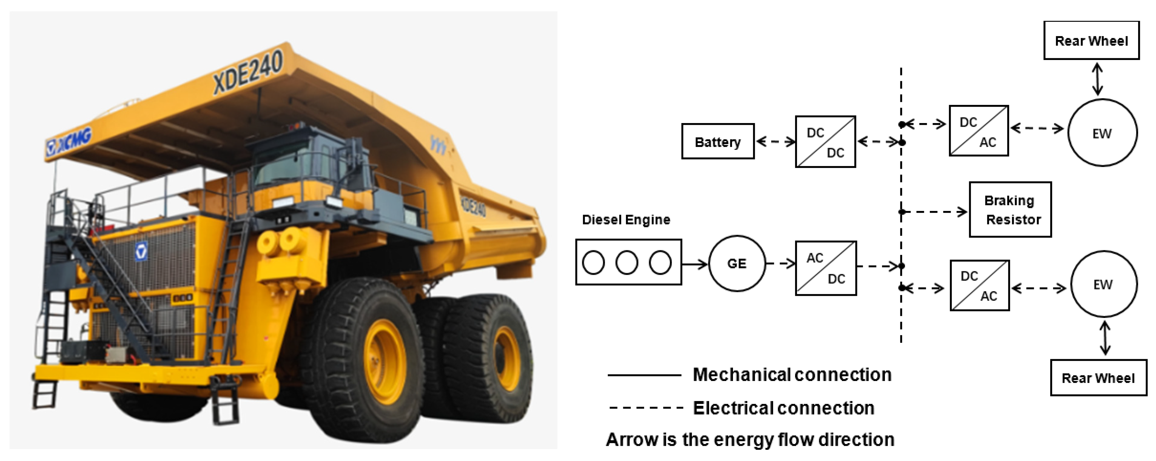
The appearance of the hybrid mining dump truck is depicted in Figure 1. To ensure that the vehicle meets the power requirements for road travel while achieving a reasonable power distribution among its power sources, the energy management strategy for the hybrid dump truck is examined. Consequently, both a discrete powertrain model and a vehicle longitudinal dynamics model are established.

2.1. SHEV Power Assembly

The series hybrid electric vehicle (SHEV) power assembly, illustrated in Figure 1, comprises an engine-generator set, a power battery, two electric wheels, and various other components. The engine is a diesel unit with a power rating of 1865 kW. The generator is a 1800 kW permanent magnet synchronous generator. The battery pack, possessing a capacity of 357 Ah, is capable of storing 440 kWh of electrical energy. The electricity produced by the generator undergoes AC/DC conversion before being connected to the DC bus alongside the power battery. The electric wheels incorporate a drive motor and a reducer. The drive motor is a three-phase permanent magnet synchronous wheel motor, which is connected to the DC bus after DC/AC conversion. The reducer functions to decrease speed and increase torque. The output power of the drive motor is transmitted to the wheels via the reducer, thereby propelling the vehicle. At time k, all powertrain components linked to the DC bus must satisfy the power balance equation, neglecting the power consumption of other electrical loads. This ensures that the system maintains an equilibrium in terms of power flow.

$$\left\{\begin{array}{l}{P}_{bat}\left(k\right)={\eta }_{req}{P}_{req}\left(k\right)-{\eta }_{eng}{P}_e\left(k\right)\\ {\eta }_{req}={\left({\eta }_{bat}{\eta }_{AC\_DC}{\eta }_{mot}{\eta }_{tran}\right)}^{-sign\left(T_{mot}\right)}\\ {\eta }_{eng}={\eta }_{AC\_DC}{\eta }_{EGS}/{{\eta }_{bat}}^{sign\left(T_{mot}\right)}\end{array}\right.$$

(1)

Here, $P_{bat}$ is the power of the battery, $P_{req}$ is the electric driving or braking power of the wheel, $P_e$ is the output power of the engine, and ${\eta }_{EGS}$ is the efficiency of the engine-generator set. Additionally, ${\eta }_{bat}$ is the charging and discharging efficiency of the battery, ${\eta }_{AC\_DC}$ is the conversion efficiency of AC/DC, ${\eta }_{mot}$ is the drive motor efficiency, and ${\eta }_{tran}$ is the transmission efficiency of the gearbox. Furthermore, $T_{mot}$ is the output torque of the drive motor, which satisfies $T_{mot}\ge 0$ during the driving status and $T_{mot}<0$ during the braking status.

In the engine-generator set model, $b_e\left(\mathrm{g}/\mathrm{kWh}\right)$ represents the fuel consumption rate of the engine. This rate can be determined from the universal characteristic curve of the engine and is influenced by the engine’s operating point, specifically its output torque and speed. The optimal fuel consumption curve of the engine is depicted in Figure 2.

$$\left\{\begin{array}{l}{P}_e\left(k\right)={\displaystyle \frac{1}{9550}}{T}_e\left(k\right)·n_e\left(k\right)\\ P_{EGS}\left(k\right)=P_e\left(k\right)·{\eta }_{EGS}\\ m_{fuel}\left(k\right)={\displaystyle \frac{\Delta t}{3600}}{\displaystyle {\sum }_{i=1}^k{P}_e\left(i\right)b_e\left(i\right)}\end{array}\right.$$

(2)

Here, $P_{EGS}$ is the output power of the engine-generator set, $T_e$ is the output torque of the engine, and $n_e$ is the engine speed. These variables must satisfy the boundary conditions of $T_e\in \left[T_{e\_\min },T_{e\_\max }\right],n_e\in \left[n_{e\_\min },n_{e\_\max }\right]$, and $P_{EGS}\in \left[P_{EGS\_\min },P_{EGS\_\max }\right]$. Here, $m_{fuel}$ denotes the fuel consumption, and $\Delta t$ represents the sampling period.

The power battery comprises multiple cells. When the ambient temperature is maintained at 25 °C and battery aging is disregarded, the relationship among the SOC of the cell, its open-circuit voltage ($U_{OC}$), and internal resistance ($R_{OC}$) is depicted in Figure 3. To estimate the SOC of the battery, an equivalent circuit model is employed, adhering to the following equations [33]:

$$\left\{\begin{array}{l}{P}_{bat}=U_{OC}·I_{bat}-I_{bat}^2·R_{OC}\\ \stackrel{·}{SOC}=-I_{bat}/Q_{bat}\end{array}\right.$$

(3)

From these, the following equation can be derived:

$$\stackrel{·}{SOC}(k)=-{\displaystyle \frac{U_{OC}(k)-\sqrt{U_{OC}{(k)}^2-4R_{OC}(k)·P_{bat}(k)}}{2R_{OC}(k)·Q_{bat}}}$$

(4)

Here, $U_{OC}$ represents the open-circuit voltage of the battery, $R_{OC}$ denotes the internal resistance, $I_{bat}$ is the battery current, and $Q_{bat}$ is the battery capacity. The charging power of the battery must satisfy the boundary condition $P_{bat\_ch}\in \left[P_{ch\_\min },P_{ch\_\max }\right]$, while the discharge power needs to adhere to $P_{bat\_dis}\in \left[P_{dis\_\min },P_{dis\_\max }\right]$. Additionally, the SOC of the battery must comply with the boundary condition $SOC\in \left[{\mathit{SOC}}_{\min },{\mathit{SOC}}_{\max }\right]$. Furthermore, $I_{bat}\ge 0$ signifies battery discharging, whereas $I_{bat}<0$ indicates battery charging.

In the drive motor model, it is crucial to account for both motor driving and braking scenarios. Consequently, there exists a disparity in the efficiency of the motor during driving and energy recovery phases. The efficiency of the drive motor can be ascertained using a lookup table, and the efficiency map of the drive motor is depicted in Figure 4. Above the 0 axis represents the driving torque, which is positive. Below the 0 axis is the braking torque, which is negative.

The output power of the driving motor must satisfy the following equation:

$$\left\{\begin{array}{l}{T}_{mot}\left(k\right)={\displaystyle \frac{T_{req}\left(k\right)}{i_g}}\\ n_{mot}\left(k\right)=i_{g}g{n}_{wheel}\left(k\right)\\ P_{mot}\left(k\right)={\displaystyle \frac{1}{9550}}{T}_{mot}\left(k\right)g{n}_{mot}\left(k\right)\\ P_{req}\left(k\right)=P_{mot}\left(k\right)g{\eta }_{tran}^{sign\left(T_{mot}\right)}\end{array}\right.$$

(5)

Here, the output torque of the drive motor, denoted as $T_{mot}$, indicates the direction of motion: a positive value signifies driving, while a negative value signifies braking. $T_{req}$ represents the torque requirement for the electric drive or braking of the wheels. The speed of the drive motor is denoted by $n_{mot}$, and $i_g$ represents the reduction ratio of the speed reducer. The wheel speed is denoted by $n_{wheel}$, and $P_{mot}$ signifies the output power of the drive motor. Additionally, ${\eta }_{tran}$ represents the transmission efficiency. The output torque $T_{mot}$ and speed $n_{mot}$ of the drive motor must lie within the following boundary conditions: $T_{mot}\in \left[T_{mot\_\min },T_{mot\_\max }\right]$ and $n_{mot}\in \left[n_{mot\_\min },n_{mot\_\max }\right]$.

2.2. Vehicle Dynamics Modeling

The specific performance parameters of the hybrid mining dump truck are outlined in

Table 1. Main parameters of the hybrid mining dump truck.

Parameters	Value	Parameters	Value
Empty weight (kg)	165,000	Driving motor max torque (Nm)	24,068
Gross vehicle weight (kg)	385,000	Engine generator set efficiency	0.94
Drive style	4 × 2	AC/DC converter efficiency	0.98
Maximum speed (km/h)	56	Rolling resistance coefficient	0.035
Max gradeability	17%	Wheel radius (mm)	1572
$\mathrm{Front} \mathrm{area} ({\mathrm{m}}^2$)	58.54	Wheel reducer ratio	31.875
Air drag coefficient	0.6	Reducer efficiency	0.96
Engine max speed (rpm)	1800	Electric generator max power (kW)	1860
Engine max torque (Nm)	10,681	Generator max speed (rpm)	1800
Driving motor max speed (rpm)	3090	Battery pack capacity	357 Ah @1237 V

. With the vehicle’s power system as the focus of our investigation, the dynamic equations governing its motion during travel are presented below [34,35]. These equations facilitate the conversion of predicted vehicle speed and slope sequences into corresponding predicted vehicle demand power sequences.

The dynamic equations are as follows:

$$\left\{\begin{array}{l}m\stackrel{·}{v}={\displaystyle \frac{T_{req}-T_{Brk}}{r}}-F_z\\ F_z=mgf·\cos \alpha +{\displaystyle \frac{1}{2}}{C}_d{A}_d\rho v^2+mg·sin\alpha \end{array}\right.$$

(6)

Here, $m$ is the total mass of the vehicle, $v$ is the vehicle’s speed, $T_{req}$ is the torque required for electric drive or wheel braking, $T_{Brk}$ is the mechanical braking torque, $r$ is the radius of the vehicle’s wheels, $F_z$ represents the driving resistance faced by the vehicle, $g$ is the acceleration of gravity, $f$ is the rolling resistance coefficient of the wheels, $\alpha$ is the slope angle, $C_d$ is the drag coefficient, $A_d$ is the windward area of the vehicle, and $\rho$ is the air density.

3. DP-MPC Strategy Based on RBF Neural Network Model Prediction

3.1. RBF Neural Network Prediction Model

The RBF neural network serves as the foundation for constructing the neural network prediction model. This model is trained using vehicle speed and road slope data from operational samples. Leveraging historical vehicle speed and slope information at the present moment, the model predicts the vehicle’s speed, slope, or required power at future time points within the prediction horizon. The RBF neural network is recognized as a typical local approximation network. Compared to the back propagation (BP) network, it boasts impressive generalization, classification capabilities, and learning efficiency. Consequently, it has found successful applications in various domains, including nonlinear function approximation, data classification, pattern recognition, image processing, system modeling, control, and fault diagnosis [36].

The employed RBF neural network adopts a three-layer feedforward architecture with a solitary hidden layer. This architecture comprises an input layer, a hidden layer, and an output layer. The network’s structure is depicted in Figure 5 [36,37,38].

(1)

RBF neural network

(1) Input layer: The input layer is used as the node of input data. Here, $x$ represents the input vector, which is denoted shown in Equation (7), and n denotes the number of neurons in the input layer.

$$x={[x_1,x_2,\cdots ,x_n]}^T$$

(7)

(2) Hidden layer: The number of neurons in the hidden layer is $p$, the activation function uses a Gaussian function to transform the input vector’s dimension space, and $\phi$ represents the vector of the kernel function:

$$\phi ={[{\phi }_1,{\phi }_2,\cdots ,{\phi }_p]}^T$$

(8)

The kernel function of each neuron is given as follows:

$${\phi }_j(x)=\exp (-{({\displaystyle \frac{‖x-c_j‖}{d_j}} )}^2) j=1,2,\cdots ,p$$

(9)

Here, $c_j$ is the central vector of the jth neuron in the hidden layer, composed of the central components of the jth neuron corresponding to all neurons in the input layer $c_j={\left[c_{j1},c_{j2},\cdots c_{jn}\right]}^T$; $d_j$ is the width vector of the jth neuron in the hidden layer, corresponding to $c_j$; and $d_j={\left[d_{j1},d_{j2},\cdots d_{jn}\right]}^T$, $‖x-c_j‖$ is the Euclidean norm, as shown in Equation (10):

$$‖x-c_j‖=\sqrt{{\displaystyle {\sum }_{i=1}^n{(x_i-c_{ji})}^2}}$$

(10)

(3) Output layer: The output layer responds to the input signal. The function of neurons in the output layer is a linear function, and the information output by neurons in the hidden layer is linearly weighted and summed to produce the output result of the entire neural network. The output of neurons in the output layer is expressed as follows:

$$\begin{array}{l}y={[y_1,y_2,\cdots ,y_q]}^T\\ y_k={\displaystyle {\sum }_{j=1}^p{w}_{kj}{\phi }_j} k=1,2,\cdots ,q\end{array}$$

(11)

Here, $q$ is the number of neurons in the output layer, and $w_{kj}$ is the weight between the kth neuron in the output layer and the jth neuron in the hidden layer.

(2)

RBF neural network prediction model

In this paper, two RBF neural network prediction models are established to forecast the future speed, slope, or required power of the vehicle based on the actual operating conditions within a mining area characterized by extended stretches of uphill and downhill roads.

Utilizing the historical speed and road slope time series data of the current vehicles as the input for the neural network prediction model, we define the input vector as $X_{in}={\left[V,\alpha \right]}^T$, where $V$ represents a sequence of historical vehicle speeds, and $\alpha$ represents a sequence of historical road slopes. At time $k$, the input vector is expressed as follows:

$$X_{in}={[V_{(k-h+1)},V_{(k-h+2)},\cdots ,V_k,{\alpha }_{(k-h+1)},{\alpha }_{(k-h+2)},\cdots ,{\alpha }_k]}^T$$

(12)

Here, $2h$ represents the vector length of the historical speed and slope data.

The output of the neural network prediction model at time $k$ is defined as $X_{out}$, and it represents the future speed and slope sequence at that moment:

$$X_{out}={[V_{(k+1)},V_{(k+2)},\cdots ,V_{(k+H)},{\alpha }_{(k+1)},{\alpha }_{(k+2)},\cdots ,{\alpha }_{(k+H)}]}^T$$

(13)

where 2H is the vector length of the predicted speed and slope data.

Assuming $f_{\alpha }$ for the nonlinear mapping function of the prediction model, we have the following:

$$X_{out}=f_{\alpha }\left(X_{in}\right)$$

(14)

Furthermore, to analyze the impact of different prediction models on the power distribution among vehicle power sources, a model is constructed to directly predict the future required power of the vehicle. The output of this neural network prediction model at time $k$ is defined as $Y_{out}$, and the required power sequence of the vehicle at that moment is expressed as follows:

$$Y_{out}={[P_{(k+1)},P_{(k+2)},\cdots ,P_{(k+H)}]}^T$$

(15)

Assuming $f_p$ to be the nonlinear mapping function of this prediction model, we have the following:

$$Y_{out}=f_p\left(X_{in}\right)$$

(16)

In the above Equations (13) and (15), H represents the prediction time horizon.

In the neural network prediction model, the training samples consist of test condition data collected from the mine, encompassing vehicle speed and slope information. The vehicle speed sample data are obtained through vehicle speed sensor tests, whereas the positional values in X, Y, and Z directions during the vehicle travel are measured using an inertial navigation system. The relative position differences of the sampling points are utilized to convert and calculate the road slope sample data. For training, 10,352 samples are used, and 2000 samples are reserved for testing.

The RBF neural network model designed for predicting both speed and slope features 2h neurons in the input layer and 2H neurons in the output layer. Alternatively, the RBF neural network model aimed at directly predicting power has 2h neurons in the input layer and H neurons in the output layer. Both prediction models assume that h and H are equal, with the number of hidden layer neurons determined using an empirical formula.

3.2. Energy Management Strategy Based on the DP-MPC Algorithm

Under working conditions where road slope information is available, two strategies employing the DP-MPC algorithm are considered: DP-MPC@v and DP-MPC@P. DP-MPC@v involves predicting future vehicle speed and road slope based on historical data of the same, calculating the future time-domain power requirements of the vehicle using a vehicle dynamics model, and then integrating this with the DP-MPC algorithm. Similarly, DP-MPC@P directly predicts the future time-domain power requirements of the vehicle using historical speed and road slope data, also incorporating the DP-MPC algorithm.

In both strategies, the predicted power requirement sequences of the vehicle in the future time domain are utilized as disturbance variables introduced into the MPC system response prediction model. This model combines with an objective function aimed at minimizing fuel consumption while maintaining SOC and ensures that all system variable constraints are met. Through the use of DP algorithm within the prediction horizon, the optimal allocation of engine and battery power sequences is obtained. The first optimal engine power in this sequence is then applied as a control variable input to the controlled object, achieving real-time control optimization of power allocation among multiple power sources for the vehicle.

The structural diagram of the DP-MPC (DP-MPC@v and DP-MPC@P) strategy is illustrated in Figure 6. The light orange dashed line represents the DP-MPC@v strategy, where the neural network model predicts future time-domain road slope and speed sequences, followed by the calculation of the vehicle’s future time-domain demand power sequence using the vehicle longitudinal dynamics model. The thick red dashed line indicates the DP-MPC@P strategy, where the neural network prediction model directly predicts the vehicle’s demand power sequence in the future time domain.

In this allocation strategy, considering the slope information of the road, in order to achieve real-time simulation of the control system, a mapping model between road distance and slope needs to be established. This model consists of discrete distance and slope points and can provide real-time feedback on road slope information during vehicle operation. The vehicle’s speed is monitored by the system in real-time, allowing for the calculation of the distance traveled by the vehicle. By combining this distance with the pre-established road distance and slope mapping model, the linear interpolation method is employed to determine the slope value of the road at any given moment for the vehicle. The current time and historical slope values, along with the vehicle’s historical speed, are utilized as input data for the neural network prediction model. This integration enables online prediction of road slope, speed, or the vehicle demand power sequence. The graphical representation of the constructed road distance and slope mapping model is depicted in Figure 7.

To fulfill the real-time control demands, a state space model for the linear discrete-time system of the SHEV system has been formulated, as illustrated in Equation (17):

$$\left\{\begin{array}{l}x\left(k+1\right)=Ax(k)+B_{u}u(k)+B_{d}d(k)\\ y(k)=Cx(k)+D_{u}u(k)+D_{d}d(k)\end{array}\right.$$

(17)

Here, $x\left(k\right)\in R^2$ represents the state vector at time k; $u(k)\in R$ is the input control vector; $y(k)\in R$ is the output vector; $d(k) \in R$ is the disturbance variable; and $A$, $B_u$, $B_d$, $C$, $D_u$, and $D_d$ are the coefficient matrices or coefficients of the equation. To ascertain the parameters within this equation, the subsequent equation is defined as follows:

$$\Delta P(k)=P_e(k)-P_e(k-1)$$

(18)

In this context, $\Delta P(k)$ denotes the difference in engine output power between time k and time $k-1$. Furthermore, Formula (4) pertaining to the battery’s SOC has been simplified according to [2], as shown in Equation (19):

$$SOC(k+1)=SOC(k)-\kappa T_s{P}_{bat}(k)$$

(19)

Here, $\kappa$ ($\kappa >0$) is a scalar parameter derived from the simulation data of the battery pack, and $T_s$ represents the sampling period.

From Equations (1)–(4), (18) and (19), the powertrain dynamics equations of a SHEV can be utilized to formulate a linear discrete system. The variables and coefficients in Equation (17) are defined as follows:

$$\begin{array}{l}y(k)=P_{bat}(k), x(k)={\left[SOC(k)P_{EGS}(K-1)\right]}^{\prime }, u(k)=\Delta P(k), d(k)=P_{req}(k),\\ A=\left[\begin{array}{cc}1& k{T}_s{\eta }_{AC-DC}/{\eta }_{bat}\\ 0& 1\end{array}\right], B_u=\left[\begin{array}{l}k{T}_s{\eta }_{eng}\\ {\eta }_{EGS}\end{array}\right], B_d=\left[\begin{array}{c}-k{T}_s{\eta }_{req}\\ 0\end{array}\right], \\ C=\left[\begin{array}{cc}0& -{\eta }_{AC-DC}/{\eta }_{bat}\end{array}\right], D_u=-{\eta }_{eng}, D_d={\eta }_{req}.\end{array}$$

Note that the state vector, input control vector, and output vector must adhere to the constraints specified in Equations (1)–(4).

At time step k, the SOC value and historical information of the hybrid system, as well as the output power and historical information of the engine-generator set at time step $k-1$, can be acquired and stored. Utilizing Equation (17), by setting N as the prediction horizon and m as the control horizon, the system response prediction equation for the DP-MPC can be derived.

$${\left\{\begin{array}{l}{X}_N\left(k+N/k\right)=S_{x}x(k)+S_{u}U\left(k\right)+S_{d}D\left(k\right)\\ Y_N\left(k+N/k\right)=C_N{X}_N\left(k+N/k\right)+D_u{\left[\begin{array}{c}U\left(k\right)\\ ⋮\\ u(k+m-1)\end{array}\right]}_{(N+1)\times 1}+D_d\left[\begin{array}{c}D\left(k\right)\\ ⋮\\ d(k+m-1)\end{array}\right]\end{array}\right.}_{(N+1)\times 1}$$

(20)

Here,

$$\begin{array}{l}{X}_N\left(k+N/k\right)\stackrel{def}{=}{\left[\begin{array}{l}x(k)\\ x(k+1)\\ ⋮\\ x(k+N)\end{array}\right]}_{(N+1)\times 1}, U\left(k\right)\stackrel{def}{=}{\left[\begin{array}{l}u\left(k\right)\\ u\left(k+1\right)\\ ⋮\\ u\left(k+m-1\right)\end{array}\right]}_{m\times 1}, D\left(k\right)\stackrel{def}{=}{\left[\begin{array}{l}d\left(k\right)\\ d\left(k+1\right)\\ ⋮\\ d\left(k+m-1\right)\end{array}\right]}_{m\times 1}, \\ S_x={\left[\begin{array}{c}\begin{array}{l}I\\ A\end{array}\\ A^2\\ A^3\\ ⋮\\ A^m\\ ⋮\\ A^N\end{array}\right]}_{(N+1)\times 1}, S_u={\left[\begin{array}{ccccc}\begin{array}{l}0\\ B_u\end{array}& \begin{array}{l}0\\ 0\end{array}& \begin{array}{l}0\\ 0\end{array}& \begin{array}{l}\dots \\ \cdots \end{array}& \begin{array}{l}0\\ 0\end{array}\\ A{B}_u& B_u& 0& \cdots & 0\\ A^2{B}_u& A{B}_u& B_u& \cdots & 0\\ ⋮& ⋮& ⋮& \ddots & ⋮\\ A^{m-1}{B}_u& A^{m-2}{B}_u& A^{m-3}{B}_u& \cdots & B_u\\ ⋮& ⋮& ⋮& \ddots & ⋮\\ A^{N-1}{B}_u& A^{N-2}{B}_u& A^{N-3}{B}_u& \cdots & {\displaystyle \sum _{i=1}^{N-m+1}{A}^{i-1}{B}_u}\end{array}\right]}_{(N+1)\times m},\end{array}$$

and

$$\begin{array}{l}{S}_d={\left[\begin{array}{ccccc}\begin{array}{l}0\\ B_d\end{array}& \begin{array}{l}0\\ 0\end{array}& \begin{array}{l}0\\ 0\end{array}& \begin{array}{l}\dots \\ \cdots \end{array}& \begin{array}{l}0\\ 0\end{array}\\ A{B}_d& B_d& 0& \cdots & 0\\ A^2{B}_d& A{B}_d& B_d& \cdots & 0\\ ⋮& ⋮& ⋮& \ddots & ⋮\\ A^{m-1}{B}_d& A^{m-2}{B}_d& A^{m-3}{B}_d& \cdots & B_d\\ ⋮& ⋮& ⋮& \ddots & ⋮\\ A^{N-1}{B}_d& A^{N-2}{B}_d& A^{N-3}{B}_d& \cdots & B_d\end{array}\right]}_{(N+1)\times m}, Y_N\left(k+N/k\right)\stackrel{def}{=}{\left[\begin{array}{l}y(k)\\ y(k+1)\\ ⋮\\ y(k+N)\end{array}\right]}_{(N+1)\times 1}, \\ C_N={\left[\begin{array}{ccccc}C& 0& 0& \cdots & 0\\ 0& C& 0& \cdots & 0\\ 0& 0& C& \cdots & 0\\ ⋮& ⋮& ⋮& \ddots & ⋮\\ 0& 0& 0& \cdots & C\end{array}\right]}_{(N+1)\times (N+1)}.\end{array}$$

Here, $S_x$, $S_u$, $S_d$, and $C_N$ are the coefficient matrix, $I$ represents the identity matrix, $U$ denotes the control variable sequence, and $D$ is the disturbance variable sequence.

To prevent rapid fluctuations in the SOC of the power battery during operation, a reference SOC trajectory should be incorporated into the DP-MPC strategy to constrain the SOC. The DP strategy, being a global optimization approach, calculates the required vehicle power based on predetermined operating conditions and a vehicle dynamic model. It establishes a global optimization objective function and a state model equation, enabling offline simulation optimization and yielding an optimal SOC trajectory for the given operating condition. Therefore, the SOC trajectory obtained from the DP strategy can serve as the reference trajectory for the battery SOC under the DP-MPC strategy, with the reference SOC value denoted as ${SOC}_{ref}$.

At time k, the recurrence formula of DP optimization solution within the MPC predictive horizon is given as follows:

$$J_k^{*}=min[{\displaystyle {\sum }_{t_k=k}^{k+N-1}[L(x(t_k),u(t_k))]+G(x(k+N))]}$$

(21)

Within the predictive horizon, for step $k+N-1$, the subproblem can be solved backward using the DP algorithm, which is expressed as follows:

$$J_{(k\_k+N-1)}^{*}x(k+N-1)=mi{n}_{u(k+N-1)}[L(x(k+N-1),u(k+N-1))+G(x(k+N))]$$

(22)

For step $k+t_k$ where $0\le t_k\le N-1$, the subproblem is expressed as follows:

$$J_{(k\_k+t_k)}^{*}x(k+t_k)=mi{n}_{u(k+t_k)}[L(x(k+t_k),u(k+t_k))+J_{(k\_k+t_k+1)}^{*}x(k+t_k+1)]$$

(23)

Here, $J_{(k\_k+t_k)}^{*}x(k+t_k)$ represents optimal objective function from the beginning of $k+t_k$ to the end of the predictive horizon, and the state variable $x(k+t_k)$ transitions to the state $x(k+t_k+1)$ in the next step under the action of the control variable $u(k+t_k)$.

To enhance the fuel economy of the vehicle and maintain the SOC within a controlled range relative to a reference trajectory, the optimization problem associated with MPC method within each predictive horizon can be articulated as follows:

$$J_k={\displaystyle {\sum }_{t_k=k}^{k+N-1}[L(x(t_k),u(t_k))]+G(x(k+N))}$$

(24)

where

$$L(x(t_k),u(t_k))=m_{fuel}(t_k)+{\lambda }_1·\Delta SOC(t_k)$$

(25)

and

$$G(x(k+N))={\lambda }_2{(SOC(k+N)-SO{C}_{ref})}^2$$

(26)

Here, $J_k$ represents the objective function within the predictive horizon, $L(x(t_k),u(t_k))$ is the instantaneous objective function, $m_{fuel}$ denotes the engine’s fuel consumption, $\Delta SOC$ is the variation of SOC, and $G(x(k+N))$ serves as a penalty function for deviations between the final SOC and the reference SOC ($SO{C}_{ref}$) at the end of the predictive horizon. The coefficients ${\lambda }_1$ and ${\lambda }_2$ effectively constrain the SOC trajectory close to the reference line, ensuring that the SOC does not fluctuate rapidly and enabling a balanced distribution of electric energy throughout the driving process.

To guarantee the normal operation of each component within the powertrain, constraint conditions must be imposed on the objective function, as illustrated in Equation (27). These conditions are formulated with a holistic consideration of both fuel economy and the durability of the power battery. Subsequently, the optimal control output sequence within the predictive horizon is obtained with a DP solution, and the first control output value $\left(P_e^{*}\left(k\right)\right)$ is then applied to the hybrid system.

$$\left\{\begin{array}{l}{P}_{e\_\min }\le P_e\le P_{e\_\max }\\ \Delta P_{\min }\le \Delta P\le \Delta P_{\max }\\ P_{ESG\_\min }\le P_{ESG}\le P_{ESG\_\max }\\ P_{dis\_\min }\le P_{bat\_dis}\le P_{dis\_\max }\\ P_{ch\_\min }\le P_{bat\_ch}\le P_{ch\_\max }\\ SO{C}_{\min }\le SOC\le SO{C}_{\max }\\ T_{mot\_\min }\le T_{mot}\le T_{mot\_\max }\\ n_{mot\_\min }\le n_{mot}\le n_{mot\_\max }\end{array}\right.$$

(27)

Here, the subscript “max” indicates the maximum value, and “min” indicates the minimum value of the corresponding physical quantity.

To summarize, the primary process of the optimal power allocation strategy based on the DP-MPC algorithm is outlined as follows:

(1)

Utilize neural network prediction models to directly or indirectly obtain the vehicle’s demand power sequence in the future time domain, which serves as the disturbance sequence. The state vector at time k is composed of the current SOC value of the power battery and the output power of the engine-generator set at time k − 1. These disturbance sequences and state vectors are introduced into the system response prediction equation of the DP-MPC framework.

(2)

Define the objective function as minimizing fuel consumption while maintaining the SOC of the battery within an acceptable range and satisfying all variable constraint conditions of the system. Using the DP solution within a prediction horizon, identify an optimal control variable sequence (engine output power) from all possible combinations of engine and power battery working states.

(3)

Apply the first value of the optimal control variable sequence as the control input to the controlled object, thereby achieving optimal power distribution among the vehicle’s multiple power sources. The operating point of the engine is determined by its speed and torque. Disregarding efficiency losses, the engine’s output power range is defined as $P_e(k)\subseteq \left\{\max (P_{req}-P_{dis\_\max },P_{e.opt}-\epsilon ),\min (P_{req}+\left|P_{ch\_\min }\right|,P_{e.opt}+\epsilon )\right\}$, where $P_{e.opt}\pm \epsilon (\epsilon \ge 0)$ is the control field on the engine’s optimal fuel consumption curve.

(4)

Utilize the real-time feedback from the vehicle system, including speed, slope, and historical information, as input data for the neural network prediction model at the subsequent time step. Repeat steps (1) through (3) iteratively to implement the rolling optimization process that is integral to the DP-MPC algorithm. Notably, the average execution time of the entire power allocation algorithm is less than 50 ms, with a sampling period of 1 s. This underscores its potential for real-time control applications.

4. Energy Management Strategy Simulation Tests

Utilizing the component, vehicle models, and neural network prediction model, the DP-MPC optimal control strategy is employed to achieve online real-time control for the hybrid mining dump truck. To assess the performance of each strategy, the impact of varying prediction horizons in the RBF neural network on prediction accuracy and fuel consumption is examined, enabling the determination of an appropriate prediction horizon. Subsequently, the performance of the studied strategies is compared with normal MPC and DP strategies.

In this investigation, the prediction horizon and control horizon of the DP-MPC strategy are aligned with the prediction horizon of the RBF neural network model. The predicted speed and slope results, depicted in Figure 8a–e, are derived from the DP-MPC@v strategy using the RBF neural network model under actual working conditions with varying slopes. The prediction time domains are set at 5 s, 7 s, 10 s, 13 s, and 15 s, respectively, with corresponding hidden layer neuron counts of 15, 22, 30, 40, and 45 in the models. Notably, prediction errors primarily arise at the peaks of speed and slope. As tabulated in

Table 2. Results of the DP-MPC@v strategy under different predictive horizons.

Predictive horizon (s)	5	7	10	13	15
RMSE of speed (m/s)	0.0550	0.0722	0.1065	0.1369	0.1438
RMSE of slope (°)	0.4552	0.6172	0.9215	1.1847	1.3343
T_step (ms)	28.36	34.63	42.41	49.50	54.20
Fuel consumption (L)	54.88	54.90	54.51	53.35	53.30

, an increase in the prediction horizon correlates with a rise in the root mean square error (RMSE) for vehicle speed and slope predictions, resulting in decreased prediction accuracy. This is attributed to the weaker correlation between long-range predictive speed and slope values and current and historical data, which hinders prediction accuracy for longer horizons. Furthermore, the modest fluctuation range of speed and slope values in the working conditions favors more precise predictions, yielding small RMSEs under operational scenarios. When the prediction time domain is set to 13 s, the vehicle’s fuel consumption is relatively low, comparable to that at 15 s, with an average step execution time of 49.50 ms, significantly less than the control system’s sampling time of 1 s. Generally, longer control horizons introduce larger prediction errors and increase computational complexity. Conversely, overly short control horizons prevent optimal control attainment. Balancing vehicle fuel consumption, real-time control capabilities, and computational efficiency, the DP-MPC@v strategy’s selection of a 13 s prediction horizon is deemed appropriate for mine operating conditions with slopes.

To analyze and compare power distribution strategies, the DP-MPC@P strategy incorporates an RBF neural network prediction model that directly forecasts the vehicle’s future power demand based on historical speed and road slope data. With a prediction time domain of 13 s and a hidden layer neuron count of 35, Figure 9a illustrates the future power demand trend for the vehicle. The black line represents actual current power demand, while the red line denotes predicted power demand. Figure 9b,c provide magnified views at 340 s and 1840 s, respectively, revealing that prediction errors are primarily concentrated at peak power demand points.

Following the evaluation framework outlined in references [2,29], the strategies’ strengths and weaknesses are assessed using indicators such as fuel economy $\left(Fuel\right)$, engine start count $\left(N_{eng}\right)$, engine output peak power $\left(P_{eng\_\max }\right)$, and average calculation time per step $\left(T\_step\right)$. Additionally, the initial $\left(SO{C}_{init}\right)$ and final $\left(SO{C}_{end}\right)$ states of charge of the power battery are considered in fuel economy calculations. $Ga{p}_{fuel}$ denotes the difference in fuel economy among the DP-MPC@v, DP-MPC@P, normal MPC, and DP strategies.

Figure 10 displays the parameter variation curves for each strategy under mine road conditions with slopes, while

Table 3. Simulation results of different strategies for the slope drive cycle.

Strategy	${\mathit{S}\mathit{O}\mathit{C}}_{\mathit{i}\mathit{n}\mathit{i}\mathit{t}}$(100%)	${\mathit{S}\mathit{O}\mathit{C}}_{\mathit{e}\mathit{n}\mathit{d}}$(100%)	${\mathit{N}}_{\mathit{e}\mathit{n}\mathit{g}}$ (n)	${\mathit{P}}_{\mathit{e}\mathit{n}\mathit{g}\_\mathit{m}\mathit{a}\mathit{x}}$ (High or Low)	$\mathit{F}\mathit{u}\mathit{e}\mathit{l}$ (L)	$\mathit{G}\mathit{a}{\mathit{p}}_{\mathit{f}\mathit{u}\mathit{e}\mathit{l}}$ (%)	$\mathit{T}\_\mathit{s}\mathit{t}\mathit{e}\mathit{p}$ (ms)
DP	0.600	0.599	11	―	51.90	―	―
DP-MPC@P	0.600	0.600	10	high	53.26	2.62	43.85
DP-MPC@v	0.600	0.600	33	low	53.35	2.79	49.50
Normal MPC	0.600	0.600	42	high	55.10	6.17	20.13

presents the performance indicator results for the evaluated strategies. Analysis reveals the following:

(1)

As depicted in Figure 10a,b, the results indicate that the engine and battery output powers of the DP-MPC@P, DP-MPC@v, and normal MPC energy management strategies remain within acceptable limits during operations on sloped terrains in mining areas. Notably, the DP-MPC@v strategy exhibits the lowest engine peak power point compared to the DP-MPC@P and normal MPC strategies, suggesting a superior control capability over engine output power. Conversely, the DP-MPC@P strategy demonstrates the smallest variation in battery’s output power compared to DP-MPC@v and normal MPC, which is favorable for extending the battery’s service life. Figure 10c,d present partial enlargements of the parameter curves for each strategy, illustrating the trends in engine and battery output power over hourly intervals.

(2)

As illustrated in Figure 10e, the SOC of the power battery controlled by the DP-MPC@P energy management strategy closely tracks the globally optimized SOC curve obtained using the DP strategy. During the simulation period of 0 to 850 s, the vehicle is in a downhill phase with the engine shut off (output power of 0 kW). The power battery discharges from 0 to 260 s and transitions to energy recovery charging from 260 to 850 s, resulting in an SOC curve that initially decreases slowly and then increases. From 850 to 2000 s, the vehicle is in an uphill phase, where the engine and power battery optimize power output distribution using the energy management strategy to enhance fuel economy.

(3)

As shown in Table 3, when compared to the DP strategy, the DP-MPC@P strategy exhibits fewer engine start-stop cycles, a slightly higher engine peak power, and a 2.62% increase in fuel consumption. In contrast, the DP-MPC@v strategy has more engine start-stop cycles, a slightly lower engine peak power, and also a 2.79% increase in fuel consumption. The normal MPC strategy, compared to the DP strategy, has the highest number of engine start-stop cycles, a slightly higher peak power, and a 6.17% increase in fuel consumption. Among the three strategies capable of real-time control, the DP-MPC@P strategy demonstrates the best performance, followed by DP-MPC@v, which outperforms the normal MPC strategy.

(4)

As indicated in Table 3, the average computation time per step for the DP-MPC@P strategy is 43.85 ms, which is 11.4% less than the 49.5 ms required by the DP-MPC@v strategy and 117% greater than the 20.13 ms of the normal MPC strategy. This is primarily attributed to the use of neural network model prediction calculations in the DP-MPC@P strategy, which increases its computational cost. However, the average computation time per step for the DP-MPC@P strategy is significantly less than the sample period of 1 s, indicating its potential for real-time control applications.

(5)

The variations in performance among the strategies can be attributed to differences in speed, slope, or power prediction models, leading to deviations in prediction results. Consequently, the calculated or predicted vehicle demand power sequences within the prediction time domain will vary, serving as disturbance variable sequences input into the system response prediction model equation. These sequences are then optimized and solved using the DP algorithm, resulting in different optimal control variable sequences and ultimately causing differences in simulation results and strategy performance.

In summary, under mining area road conditions with slopes, a strategy is proposed that directly predicts future vehicle power demand based on speed and slope, combined with the DP-MPC algorithm (DP-MPC@P). This strategy reduces the fuel consumption cost of the entire vehicle, aligns the SOC curve change of the battery more closely with the SOC trajectory of the DP strategy, and exhibits superior overall performance. The DP-MPC@P strategy demonstrates excellent optimal control performance in the energy management of hybrid mining dump trucks, with overall performance close to that of the DP strategy.

5. HIL Experiments

In the preceding sections of this paper, the construction and simulation of the DP-MPC energy management strategy, which is grounded in condition prediction, have been successfully completed. To validate the real-time performance and robustness of this energy management strategy, a HIL test platform is established based on the offline simulation results, and subsequent HIL testing research is conducted.

The HIL testing platform has been constructed, as depicted in Figure 11. The platform comprises the following components: an NI PXI rack, a PC upper computer, a vehicle control unit (VCU, MPC5744), and the VeriStand control platform. Specifically, the NI PXI rack provides a real-time vehicle environment. The PC upper computer, connected to the NI PXI hardware via Ethernet, is responsible for downloading simulation models to the NI PXI and deploying them into the real-time system. The VeriStand 2017 experiment management software sets up the test environment (test project) and controls the test system execution. Meanwhile, the Kvaser USBCAN, based on the D2P development platform, flashes the compiled control strategy srz file into the VCU.

The primary steps involved in creating the HIL test system are outlined as follows: (1) Configure the real-time target machine and deploy (download) the developed test project onto the real-time machine (also referred to as the lower computer). (2) Integrate NI series equipment into the VeriStand environment. Specifically, the following devices should be incorporated: those equipped with a PXI-7841R board, a CAN communication board (PXI-8512/2), and a programmable power supply. Additionally, the CAN bus communication channel is configured with a baud rate of 500 kbps. (3) Incorporate the controlled object model into the test engineering framework. (4) Once the hardware and software resources have been added, adjust the connection port mapping accordingly, utilizing a provided mapping file to ensure the alignment of project signals.

The FTP-75 standard driving cycle with a scaled-down speed ratio is utilized for the flat terrain scenario, while actual mining road conditions represent the graded terrain scenario. To validate the real-time performance and robustness of the DP-MPC@P energy management strategy, HIL tests were conducted under both scenarios, with the initial and final SOC of the traction battery set at 0.6. Figure 12a,b illustrate the speed tracking of the actual vehicle speed versus the target vehicle speed for the flat and graded terrain scenarios, respectively. It is evident from these figures that the DP-MPC@P strategy achieves excellent speed tracking performance under both conditions. Figure 12c,d demonstrate that, under both scenarios, the traction battery can charge and discharge normally within the allowable range, enabling the engine to operate at higher efficiency. The dashed boxes in the vehicle demand power plots indicate negative power values due to mechanical braking when the vehicle speed falls below a set threshold. The solid boxes show negative power values less than the battery’s maximum energy recovery capacity, with excess energy dissipated as heat by braking resistors. Therefore, it can be observed that the combined power of the engine and battery, as regulated by the proposed strategy, is sufficient to meet the vehicle’s anticipated power requirements, thereby ensuring dynamic vehicle performance. The simulation results indicate that the DP-MPC@P strategy achieves satisfactory control outcomes under various driving conditions.

6. Conclusions

To optimize the energy distribution strategy for a multi-power source large mining hybrid dump truck and enhance its fuel economy under practical working conditions featuring slopes in mining areas, this paper introduces a DP-MPC@P strategy that leverages historical speed and road slope data. This strategy directly predicts the vehicle’s required power using a RBF neural network and effectively integrates the DP-MPC algorithm, enabling energy allocation management and online real-time optimization control. The key findings are as follows:

(1)

The predictive accuracy of the RBF neural network for vehicle speed and slope diminishes as the prediction time domain increases. Under mining scenarios with slopes, vehicle speed and slope predictions are conducted across five prediction time domains. Taking into account factors such as fuel consumption, real-time control, and computational efficiency, the optimal prediction time domain for the neural network model in the DP-MPC@v strategy is determined to be 13 s. To facilitate a comparative analysis of strategy performance, the prediction horizon for the DP-MPC@P strategy is similarly set at 13 s.

(2)

Various strategies are compared and validated under mining conditions with slopes. The DP strategy yields the lowest fuel consumption (51.90 L) and minimal engine start-stop cycles (11 times). In contrast, the normal MPC strategy consumes 55.10 L of fuel and experiences 42 engine start-stops. The DP-MPC@P strategy reduces fuel consumption by 3.34% (to 53.26 L) and engine start-stops by 76.2% (to 10 times). Compared to the DP-MPC@v strategy, which consumes 53.35 L of fuel and has 33 engine start-stops, the DP-MPC@P strategy exhibits slightly lower fuel consumption (53.26 L) and a 69.7% reduction in engine start-stops (to 10 times). These results indicate that the DP-MPC@P strategy exhibits superior fuel economy and control performance.

(3)

The DP-MPC@P strategy achieves an average computation time per step of 43.85 ms, which is 11.4% less than the DP-MPC@v strategy’s 49.5 ms. This efficiency is attributed to the DP-MPC@P strategy’s neural network prediction model, which features a simpler structure with fewer output layer neurons and avoids recalculating the demand power sequence with the vehicle dynamics model. Consequently, the DP-MPC@P strategy’s average computation time per step is significantly less than the 1-second sample period, enabling online real-time control.

(4)

The offline simulation results of MATLAB R2022a version align closely with HIL test results under both the scaled speed FTP-75 standard cycle without slopes and actual mining road conditions with slopes. This consistency validates the DP-MPC@P strategy’s real-time performance and robustness, suggesting its potential application in hybrid electric vehicle energy management systems.