Neural-Driven Constructive Heuristic for 2D Robotic Bin Packing Problem

Abstract

This study addresses the two-dimensional weakly homogeneous Bin Packing Problem (2D-BPP) in the context of robotic packing, where items must be arranged in a manner feasible for robotic manipulation. Traditional heuristics for this NP-hard problem often lack adaptability across diverse datasets, while metaheuristics typically suffer from slow convergence. To overcome these limitations, we propose a novel neural-driven constructive heuristic. The method employs a population of simple feed-forward neural networks, which are trained using black-box optimization via the Covariance Matrix Adaptation Evolution Strategy (CMA-ES). The resulting neural network dynamically scores candidate placements within the constructive heuristic. Unlike conventional heuristics, the approach adapts to instance-specific characteristics without relying on predefined rules. Evaluated on datasets generated by 2DCPackGen and real-world logistic scenarios, the proposed method consistently outperforms benchmark heuristics such as MaxRects and Skyline, reducing the average number of bins required across various item types and demand ranges. The most significant improvements occur in complex instances, with up to 86% of 2DCPackGen cases yielding superior results. This heuristic offers a flexible and extremely fast, data-driven solution to the algorithm selection problem, demonstrating robustness and potential for broader application in combinatorial optimization while avoiding the scalability issues of reinforcement learning-based methods.

1. Introduction

Efficiently solving packing problems is crucial for many industrial and robotic applications, where space utilization and automation are critical. This paper focuses on a specific variant, the two-dimensional robotic bin packing problem with weakly heterogeneous items. We consider the problem of packing two-dimensional rectangle items $i\in \mathbf{I}$ into a set of large objects, referred to as bins throughout this paper. Each bin is a rectangle with width W and height H. An item $i\in \mathbf{I}$ has width $w_i$ and height $h_i$ (height $h_i$ does not have to be larger than width $w_i$). We assume a weak heterogeneity among the items, meaning that items can be grouped into relatively few types compared to the total number of items. Let $\mathbf{T}$ denote the set of types of items. For each type $t\in \mathbf{T}$, all items are collected in the set ${\mathbf{I}}_t$ and share identical width and height. Each item must be placed orthogonally within a bin, must not extend beyond the bin’s boundaries, and must not overlap with another item. In addition, the packing must be robotic, which means that a feasible robot motion exists to place each item in the bin. An item can be inserted into the bin from one of its sides: vertically or horizontally. The objective is to minimize the number of bins required to pack all the items.

Table 1. Problem notation.

Notation	Meaning	Notation	Meaning
W	Width of a bin	H	Height of a bin
$\mathbf{T}$	Set of item types	$t\in \mathbf{T}$	Index of an item type
$\mathbf{I}$	Set of all items	$i\in \mathbf{I}$	Index of an item
${\mathbf{I}}_t$	Set of all items of type t
$w_i$	Width of item i	$h_i$	Height of item i

summarizes the problem notation, and Figure 1 illustrates the problem representation with an example.

In principle, the assumption of weak heterogeneity is not essential. However, it strongly stems from practical considerations (see logistic dataset introduced in Section 4.2.2). Recognizing this, we aim to leverage the knowledge inherent in the data to solve 2D-BPPs exhibiting this characteristic more effectively.

Although we formulate the problem in terms of packing items into bins, it is well known that packing and cutting problems share the same structural foundation. Specifically, the problem we consider is recognized as the 2D Cutting Stock Problem (CSP) in Wäscher’s typology of cutting and packing problems [1], with the additional assumption that the cuts are not guillotine. The closest related packing problem is the Bin Packing Problem (BPP), which differs mainly in assuming strongly heterogeneous items.

This problem has numerous applications, particularly in industries involving robotic systems. Industry 4.0 is characterized by the convergence of cutting-edge technologies, with robotic packing solutions emerging as a key trend in logistics [2]. In this context, planning and managing robotic movement heavily relies on efficient packing strategies. For instance, autonomous pallet collection requires layer-by-layer packing in a manner that enables robotic arm maneuvering (so-called robotic packing), which is crucial in robotic palletization [3]. Similarly, automated warehouse systems require optimized packing strategies when preparing shipping boxes for customers, ensuring that the packing plan is executable by a robotic system [4]. The integration of packing problems and robotics is an emerging field in the literature [5]. Since packing and cutting problems are equivalent, robotic cutting of materials is equally important. The CSP applications span multiple industries, including paper manufacturing [6], glass panel cutting [7], wood processing [8], construction [9], and network traffic scheduling [10], many of which operate in robotic environments requiring movement planning and maneuvering.

While 3D bin packing is the ultimate goal for many robotic packaging systems, the 2D bin packing problem is highly relevant, as it provides foundational algorithms, supports layer-based packing, and simplifies testing and computation. In many robotic packaging systems, such as palletizing or conveyor-based packing, items are arranged in layers or on flat surfaces (e.g., boxes on a pallet or items in a tray). For example, in e-commerce warehouses, robots often pack items into flat shipping boxes or totes, where height is less variable, making 2D packing algorithms directly applicable. Moreover, 3D bin packing can often be broken down into a series of 2D packing problems. In practice, robotic systems may pack items in stable layers, stacking them to fill a 3D container. Each layer can be treated as a 2D packing problem, and optimizing these layers directly contributes to efficient 3D packing.

The Cutting Stock Problem is NP-hard (Non-deterministic Polynomial-time hard), making exact approaches impractical for large instances. As a result, heuristics and metaheuristics are widely used [11]. However, traditional metaheuristic approaches, such as genetic algorithms, simulated annealing, and variable neighborhood search, suffer from slow convergence and lack of knowledge retention—each time they are executed, they restart the search process from scratch without leveraging previous experience. This means that it repeatedly explores a vast search space and evaluates numerous partial solutions—many of which ultimately lead to dead ends. This redundancy could be mitigated by skipping moves that historically (on average) do not contribute to good solutions. Moreover, heuristics and metaheuristics are not universally effective, as their performance varies across different datasets, and therefore, it is impossible to select the best heuristics. Another key challenge is that metaheuristics are prone to being trapped in local optima.

In this paper, we propose a novel constructive approach to solving the CSP. Our method mitigates the inefficiencies of repetitive searches in metaheuristics by leveraging prior knowledge of expected data characteristics, which is commonly available in many practical scenarios. Our approach can also be interpreted as a dynamic heuristic selection method. It evaluates potential item placements at each step, selecting the most promising one from a superset that encompasses placements proposed by a broad range of heuristics. Our contributions can be summarized as follows:

• We introduce a new constructive heuristic for the CSP that incorporates data characteristics during the packing process.
• Our algorithm is based on a simple neural network used to evaluate possible steps in solution construction. Unlike many neural network-based approaches for packing and cutting problems, our method is independent of problem size, specifically the size of the definition of the current partial packing, which varies along with the packing items.
• We integrate machine learning with a constructive heuristic framework, leading to a black-box optimization of neural network parameters. Due to the neural network’s simplicity, we can tackle a population of networks efficiently during the training. Our method overcomes key limitations of existing approaches, providing a more adaptive and efficient solution to the CSP.
• We provide an extremely fast method compared to metaheuristics and most deep-reinforcement learning methods (less than 3 ms computational time for the largest problems). That can be crucial for real applications in the case of robotic packing when problem data change and rapid response is crucial.
• We conduct a systematic evaluation using datasets provided by 2DCPackGen [12] and real-world data from the fast-moving consumer goods (FMCG) industry, demonstrating that our approach outperforms traditional constructive heuristics.

The rest of this paper is structured as follows. Section 2 reviews the state of the art in the cutting stock problem. Section 3 formally defines the problem and provides a detailed description of our neural-driven constructive heuristic. Numerical experiments comparing proposed algorithms with known heuristics are presented in Section 4. Finally, Section 5 summarizes our findings and presents final conclusions.

2. Related Literature

The 2D Cutting Stock Problem (2D-CSP) and the 2D Bin Packing Problem (2D-BPP) can be formulated as Mixed Integer Linear Programming (MILP) models [13,14] and solved using exact methods such as branch-and-price, column generation, or Benders decomposition [15]. However, due to their combinatorial nature, exact algorithms scale exponentially with problem size, making heuristics and metaheuristics the preferred approach for practical applications.

Numerous metaheuristic algorithms have been proposed, including large neighborhood search [16], genetic algorithms [17], and ant colony optimization [18]. However, these methods often suffer from slow convergence.

Traditional heuristic approaches typically decompose the problem into two subtasks: (1) sequencing the items, and (2) determining their placement. Most research has concentrated on the placement problem, often assuming a predefined ordering of items or evaluating multiple orderings based on specific item characteristics, such as descending size.

For placement, key heuristics include Corner Points [19], Extreme Points [20], MaxRects [21], or Empty Maximal Space in 3D problems [22]. These heuristics are a representation of the current state of the packing and generate potential placements. The Skyline algorithm, which traces only the top envelope of packed items, simplifies the envelope-based approach used in Corner Points and Extreme Points heuristics [23]. In contrast, approaches such as shelf and guillotine algorithms partition the bin using horizontal or guillotine cuts, while MaxRects employs overlapping rectangles to improve space utilization [21].

The selection of a placement is typically conducted in a greedy manner, guided by a scoring function. Widely used selection rules include Bottom-Left and Best-Fit heuristics [24,25], Best Short Side Fit [21], and Occupied Area Ratio [26].

There is no universally optimal heuristic, as different heuristics perform better for different datasets. This issue, known as the Algorithm Selection Problem, was first introduced by Rice [27]. Some studies attempt to learn the best heuristic based on problem instances. For example, Jipan applied a genetic algorithm to optimize coefficients for a linear combination of greedy heuristics, improving performance in 93% of 2D Bin Packing Problem instances with certain input distributions [28]. Similarly, Rakotonirainy used data mining techniques in the strip packing problem, building a dataset of solved instances to predict the best heuristic for a given input [29].

The hyper-heuristic approach aims to select or combine multiple heuristics dynamically. Beyaz et al. proposed a hyper-heuristic framework for 2D packing problems inspired by evolutionary algorithms, using crossover and mutation operators to optimize heuristic selection [30].

Recently, machine learning (ML) has gained attention in the context of cutting and packing problems. However, 2D cutting and packing problems have received surprisingly little attention compared to 1D-BPP [31] or 3D-BPP [32]. Most studies addressing 2D-BPP focus on irregular item packing rather than the standard rectangular case [33].

Some approaches treat the packing space as a discretized grid, allowing reinforcement learning (RL) to make placement decisions. However, these methods struggle with scalability [34]. More advanced end-to-end deep RL techniques, such as a modified Pointer Network with an attention module, have been proposed to enhance learning-based packing solutions [35].

Several studies attempt to integrate heuristics with deep learning. For example, Yang et al. used deep RL for online 3D bin packing, leveraging heuristics to generate feasible actions, which were then selected by the neural network agent [36]. In [37], heuristics were incorporated into the reward function within an RL framework to guide learning. Zhao et al. introduced a tree-based representation for 3D packing, where heuristics expand the tree, and deep RL learns a policy for selecting nodes during solution construction [38].

Additional insights come from the related strip packing problem, where ML techniques are used to guide heuristic selection. For instance, Fang et al. proposed a pointer network with an encoder-decoder architecture to optimize packing sequences, integrating it with MaxRects-BL for placement [39]. Similarly, Xu et al. introduced a dual graph neural network, where one network selects the next item to pack while the other encodes the free space geometry [40]. Álvaro et al. applied supervised learning for problem classification, enabling the recommendation of an appropriate heuristic based on instance characteristics [41]. Kai Zhu et al. combined a neural network with reinforcement learning, using it as a scorer to evaluate placement candidates dynamically [42]. The concept we propose in this paper has been successfully applied to the Strip Packing Problem [43].

Table 2. Literature overview.

Ref.	Authors	Date	Problem	Proposed Solutions
Exact methods
[13]	Carvalho et al.	2002	2D-CSP, 2D-BPP	Liner programming formulations (branch-and-price, column generation)
[14]	Silva et al.	2010	2D-CSP, 2D-BPP	Integer programming
[15]	Cote et al.	2021	2D-BPP	Benders decomposition
Metaheuristics
[16]	Ekici	2003	2D-BPP	Large neighbor search
[18]	Tang et al.	2021	2D-BPP	Ant colony optimization
[17]	Correia et al.	2025	2D-BPP	Genetic algorithms
Heuristics
[24]	Baker et al.	1980	2D-BPP	Bottom-Left heuristic
[19]	Martello et al.	2000	2D-BPP	Corner Points heuristic
[25]	Burke et al.	2004	2D-BPP	Best-Fit heuristic
[20]	Crainic et al.	2008	2D-BPP	Extreme Points heuristic
[21]	Jylänki	2010	2D-BPP	MaxRects heuristic
[23]	Wei et al.	2011	2D-BPP	Skyline algorithm
[26]	Da Silveira	2013	2D-BPP	Occupied Area Ratio heuristic
[22]	Ha et al.	2017	3D-BPP	Empty Maximal Space heuristic
Algorithm selection
[27]	Rice	1976	Algorithm Selection Problem	Introduced algorithm selection concept
[30]	Beyaz et al.	2015	2D-BPP	Hyper-heuristic with evolutionary operators
[42]	Zhu et al.	2020	Strip Packing	Neural network scorer for placement evaluation
[29]	Rakotonirainy	2021	Strip Packing	Data mining for heuristic selection
[41]	Neuenfeldt Júnior et al.	2023	Strip Packing	Supervised learning for heuristic selection
[39]	Fang et al.	2023	Strip Packing	Pointer Network + MaxRects-BL heuristic
[28]	Huang	2024	2D-BPP	Genetic optimization of heuristic weights
Machine learning
[37]	Yang et al.	2021	3D-BPP	RL framework
[33]	Fang et al.	2021	2D-BPP (irregular items)	Hybrid Reinforcement Learning
[38]	Zhao et al.	2022	3D-BPP	Tree-based RL-guided solution building
[31]	Guerriero et al.	2023	1D-BPP	RL with a new reward concept
[32]	Que et al.	2023	3D-BPP	RL with transformer network
[34]	Kaleta et al.	2024	2D-BPP	RL with discretized grid
[36]	Yang et al.	2024	3D-BPP	Deep RL with heuristic-guided actions
[40]	Xu et al.	2024	Strip Packing	Dual Graph Neural Network (item and space)
[35]	Wang et al.	2025	2D-BPP	Deep RL with Pointer Networks
[43]	Sliwinski et al.	2025	Strip Packing	Neural-driven constructive heuristic

provides a summary of studies within the bin packing literature, particularly focusing on algorithm selection and machine learning approaches.

To the best of our knowledge, there is limited research on applying reinforcement learning to constructive heuristics for 2D cutting stock and bin packing problems. We identify the following research gaps:

• There is no systematic framework for selecting the most suitable heuristic for specific instances of 2D-CSP and 2D-BPP.
• The potential of machine learning for heuristic selection in these problems remains largely unexplored. No prior studies have investigated data-driven deep learning approaches to discover correlations between instance characteristics and optimal heuristics.
• Existing heuristic selection approaches primarily rely on static decisions, where a chosen heuristic remains fixed throughout the solution process.
• A key challenge in constructive algorithms is the variable decision space at each step, making direct application of reinforcement learning difficult.

In this paper, we propose a novel framework for 2D cutting and packing problems that dynamically scores candidate placements, encompassing placements proposed by a wide range of heuristics. Unlike traditional reinforcement learning, we propose a population-based learning process using multiple simple neural networks, each acting as a scorer during the construction of the solution. Thus, each network implicitly represents a heuristic, potentially discovering entirely new placement strategies. Since this method generalizes considered heuristics, there is no longer a need to choose the best heuristic explicitly. Instead, knowledge is extracted from data in a context-aware manner.

3. Materials and Methods

3.1. Constructive Heuristics

Our approach is based on the general principle of constructive heuristics, which iteratively builds a solution. Let $h\in \mathbf{H}$ represent a specific heuristic from the set of all possible constructive heuristics $\mathbf{H}$, where each heuristic satisfies the assumptions outlined in this section. For instance, the set $\mathbf{H}$ includes all variants of MAXRECTS heuristics [21], Skyline heuristics [23], but also heuristics based on Corner Points and Extreme Points [19,20]. However, this set is defined in a generic sense and can also encompass other potential constructive heuristics, including those not yet known. A constructive heuristic h starts with an initial solution $s_0$, i.e., an empty bin and all items $\mathbf{I}$ to be packed, and iteratively chooses an item and its placement in a bin, possibly adding a new bin. The notation related to the general and neural-based constructive heuristic algorithm, along with explanations of the terms used, is compiled in

Table 3. Constructive heuristic notations.

Notation	Meaning
$\mathbf{H}$	Set of all constructive heuristics
$h\in \mathbf{H}$	A specific constructive heuristic
$\mathbf{S}$	Set of all possible partial solutions
$s_0$	Initial partial solution (empty bin and all items)
$s_k\in \mathbf{S}$	Partial solution after placing $k-1$ items
${\mathbf{I}}_k\subseteq \mathbf{I}$	Remaining items to be packed at iteration k
$\mathbf{D}$	Set of all possible decisions
${\mathbf{D}}_k$	Set of feasible decisions at iteration k
$d\in {\mathbf{D}}_k$	A feasible decision at iteration k
$i\left(d\right)$	Item selected in decision d
$l_{i\left(d\right)}$	Location (coordinates) for placing item $i\left(d\right)$
$r_{i\left(d\right)}$	Boolean indicator of rotation (true if rotated) of item $i\left(d\right)$
$T:(\mathbf{S},\mathbf{D})\to \mathbf{S}$	Transition function updating the solution with a decision
$p_h:(\mathbf{S},\mathbf{D})\to {\mathbb{R}}^m$	Property function mapping state and decision to feature vector
$E_h\left(p_h(s_k,d)\right)$	Evaluation function scoring properties of decision d at partial solution $s_k$
$N_{\overline{w}}$	Neural network with weights $\overline{w}$
$\overline{w}$	Vector of all trainable weights in neural network

.

At the beginning of the k-th iteration, $k=1,2,\cdots$, the current partial solution is denoted as $s_k\in \mathbf{S}$, where $s_k$ represents the packing configuration after placing $k-1$ items, and the remaining items to be packed are denoted by $I_k\subseteq I$. The set $\mathbf{S}$ contains all possible partial solutions, i.e., all possible packings of any subset of items.

In iteration k, a new item must be chosen, possibly rotated, and placed into a bin. Let $d\in {\mathbf{D}}_k\subseteq \mathbf{D}$ denote a potential decision in iteration k, where ${\mathbf{D}}_k$ is the set of all feasible decisions given the current partial solution $s_k$, and $\mathbf{D}$ is the set of all possible decisions across any partial solution. Decision d is a triplet $(i\left(d\right),l_{i\left(d\right)},r_{i\left(d\right)})$, where $i\left(d\right)\in I$ denotes the item chosen in decision d, $l_{i\left(d\right)}$ is its location (e.g., coordinates of its bottom left corner), and $r_{i\left(d\right)}$ is a boolean indicator of item i rotation (item non-rotated or rotated by 90 degrees).

Each decision made by a constructive heuristic transforms the current partial solution into an updated solution. This transformation is represented by a function:

$$T:(\mathbf{S},\mathbf{D})\to \mathbf{S}$$

(1)

where $T(s_k,d)$ adds one item according to the decision $d\in {\mathbf{D}}_k$ to the current packing $s_k$, producing a new partial or final solution, $s_{k+1}$.

The selection of an item and its placement is specific to each constructive heuristic $h\in \mathbf{H}$ and is guided by heuristic rules or criteria, which are typically chosen based on prior knowledge or computational experiments. These criteria often take into account the item’s properties (e.g., width, height) and/or characteristics of the current packing state (e.g., wasted space).

Let

$$p_h:(S,D)\to {\mathbb{R}}^m$$

(2)

denote a property function that assigns an m-dimensional vector to a partial solution $s_k$ and a candidate decision d under heuristic $h\in \mathbf{H}$. Typical properties considered in the bin packing problem include item size, aspect ratio, and space utilization.

Each heuristic h evaluates a decision d based on properties $p_h$ and greedily selects the decision that maximizes the evaluation function:

$$E_h\left(p_h(s_k,d)\right):{\mathbb{R}}^m\to {\mathbb{R}}^1$$

(3)

where $E_h\left(p_h(s_k,d)\right)$ assigns a scalar score to the decision d at state $s_k$. For instance, if $p_h(s_k,d)$ computes the item’s area and the wasted space after the placement, the heuristic might choose the largest item and place it at the position that minimizes wasted space.

The generic constructive heuristic algorithm $h\in \mathbf{H}$ follows these steps:

• Initialize: Set $k:=0$ and initialize set of items ${\mathbf{I}}_k:=\mathbf{I}$, and the partial solution $s_0$ (empty bin).
• Start an iteration: Set $k:=k+1$
• Select a Decision: Find the decision ${\widehat{d}}_k$ that maximizes the evaluation function E:

  $${\widehat{d}}_k:=arg\underset{d\in D_k}{max}{E}_h\left(p_h(s_k,d)\right)$$
• Update Solution: Apply the decision ${\widehat{d}}_k$ to extend the current partial solution:

  $$s_{k+1}:=T(s_k,{\widehat{d}}_k)$$
• Update set of items: Remove newly inserted item $i\left({\widehat{d}}_k\right)$ from the set of items to pack:

  $${\mathbf{I}}_{k+1}:={\mathbf{I}}_k\setminus \left\{i\left({\widehat{d}}_k\right)\right\}$$
• Iterate: If there are still items to pack, start a new iteration from step 2. Otherwise, stop.

Constructive heuristics typically rely on a limited set of item properties and features of the current partial solution. In most cases, these heuristics consider only one property of the item and one characteristic of the partial solution at a time. For example, the Maximal Rectangles Bottom-Left (MAXRECTS-BL) heuristic determines placement based on the x and y coordinates of all possible positions [44]. The evaluation function, denoted as E, selects the placement with the smallest y-coordinate, and if multiple positions share the same y-value, the smallest x-coordinate is used as a tiebreaker. However, different properties perform better for different problem instances, making it impossible to identify a single best heuristic $h\in \mathbf{H}$.

Furthermore, the function E, which evaluates and prioritizes different placement options, is usually defined by simple, static rules that dictate item selection, placement, and orientation. For example, the MaxRects heuristic orders items based on predefined criteria such as descending area, descending perimeter, aspect ratio, or the difference between rectangle sides. Similarly, placement decisions follow rigid selection rules, including:

• Bottom-Left: selecting the position that minimizes the y-coordinate of the top side.
• Best Area Fit: choosing the smallest available space.
• Best Long Side Fit: placing the item where the longest remaining side is minimized.

Once these sorting and placement strategies are defined, they remain fixed throughout the entire algorithm execution, without adapting to the current partial solution. This rigid approach means that the effectiveness of a given heuristic can vary significantly across different problem instances, depending on the characteristics of the input data.

3.2. Concept of New Neural-Driven Heuristics

Observations we stated in the previous section led us to formulate the following expectations for the new heuristic:

• It should incorporate a broader set of properties from the current partial solution and dynamically adjust the relevance of these properties based on the specific problem instance.
• It should enable an adaptive decision-making for item selection, orientation, and placement, allowing the heuristic to evolve as the solution is constructed.

The core concept of our approach is to replace the traditional evaluation function E with a neural network, which learns to assess the properties of available alternatives regarding items and their placements at each step of the constructive heuristic. This neural network identifies which features are most important in a given context and determines which item, placement, and orientation decisions contribute to an optimal solution.

Unlike conventional heuristics that follow predefined rules, our model evaluates each alternative separately based on the current partial solution. This makes it possible to handle a variable number of candidate placements while maintaining a fixed-size input representation for the neural network.

The input to the neural network is a vector of properties, denoted as $p_h(s_k,d)\to {\mathbb{R}}^m$, where:

• $s_k$ represents the current state of the partial solution,
• $d\in \mathbf{D}$ denotes a candidate decision,
• m is the number of considered properties, which is expected to be larger than those used in conventional heuristics.

In the most general case, the decision space ${\mathbf{D}}_{\mathbf{k}}$ of the construction heuristic for the bin-packing problem is huge. That means an item can be placed all over the empty space of bins. To make it computationally feasible, we decided to limit the set of possible placing positions to certain, sensible alternatives. In the algorithm proposed by Martello et al. [19], the authors utilize a set of placing positions called Corner points. These are non-dominated locations, where the envelope of items already in the bin changes from horizontal to vertical, see Figure 2.

Although there is no guarantee that the optimal solution to every problem can be constructed by placing properly ordered items in the right Corner points (see [20,45]), we show in the next section that this approach gives very good results when combined with the proposed neural-driven construction heuristic. Moreover, the use of Corner points ensures robotic packing. Due to the definition of Corner points as a breaking point of the envelope, it is always possible to insert an item from two sides.

In general, there are four decision types to be made: which item, rotated or not, at which bin, and which position within that bin. However, for the bin selection, we assume that only one bin is opened at a time. A bin is closing and a new bin is opened only if none of the remaining small items fit in an already opened bin.

At step k, a neural network $N_{\overline{w}}$ with weights $\overline{w}$ is used to score all item types still available for placement in their original and rotated versions and all feasible Corner points in an opened bin. So, the decision ${\widehat{d}}_k$ is to choose a triplet consisting of an item type, its rotation, and a placement position that maximizes the evaluation $N_{\overline{w}}\left(p_h(s_k,d)\right)$. 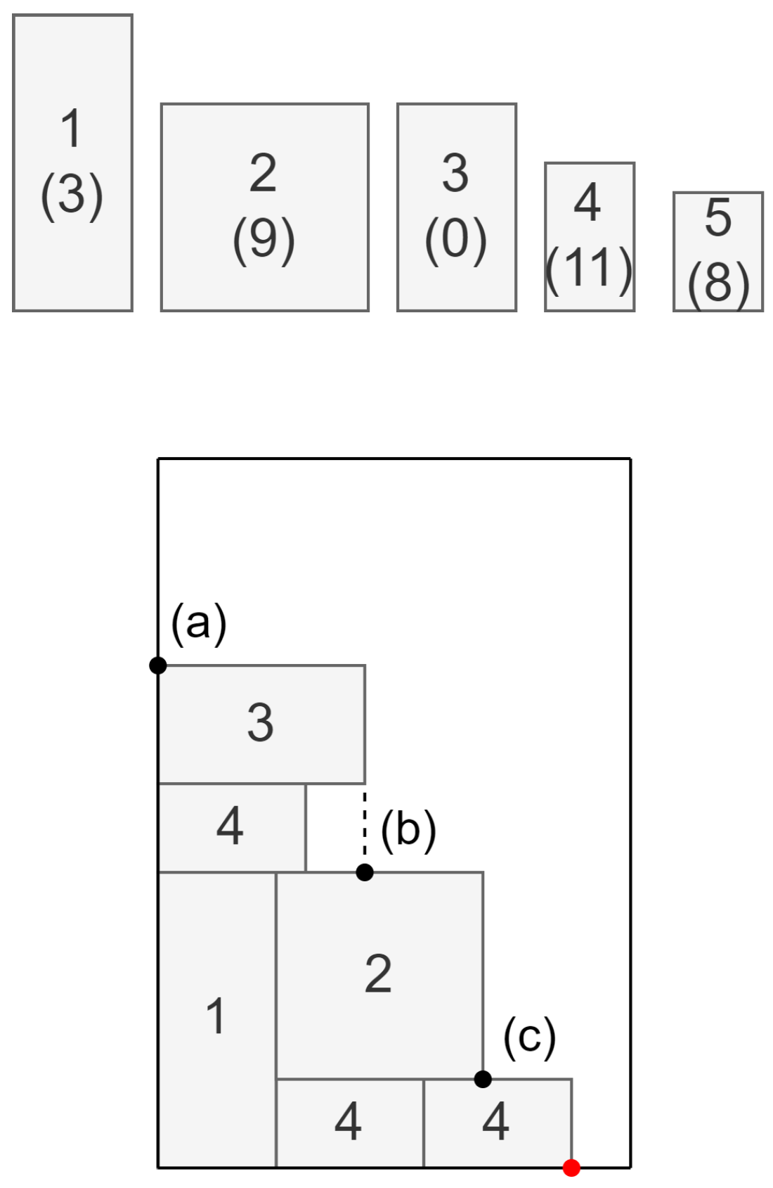For example, in the situation depicted in Figure 3, item types are illustrated at the top of the figure. The number of items of a given type to be packed is shown in parentheses, which means there are no more items of type 3. Therefore, four item types (1, 2, 4, and 5), each in two possible rotations, together with three Corner points (a–c) (the leftmost corner point highlighted with red color is ruled out, as the accompanying free space is smaller than any of the dimensions of the small items), are under consideration. Thus, the total number of alternative decisions equals $4·2·3=24$. Each decision is checked against its feasibility. For example, placing element type 1 rotated by 90 degrees at the Corner point (c) is not possible since the element would protrude beyond the bin. For each feasible combination, the properties $p_h(s_k,d)$ of the partial solution $s_k$ and each decision d are evaluated by the neural network $N_{\overline{w}}$.

As discussed later in this section, our algorithm applies a population of neural networks for training purposes. That implies the evaluation procedure should be very efficient. Therefore, we use a small-scale and simple feed-forward neural network for $N_{\overline{w}}$ with an architecture depicted in Figure 4. The network has a four-layer architecture with 24 inputs and 1 output. While the output is a numerical evaluation, the inputs are discussed in depth in the following subsection. The hidden layer sizes are 32 and 16, respectively. The hidden layers and the output are equipped with bias values. Only hidden layers utilize the tanh activation function. The total number of network parameters (weights) is 1345. Initially, all the weights are set to 0.

The output of the neural network is a scalar evaluation score, which quantifies the quality of each possible decision $d_k$ given the current state $s_k$. A higher score indicates a better placement decision. However, this value does not have an explicit probabilistic interpretation—it is solely used to rank and select the best available placement at each step.

The overall solution construction process is illustrated in Figure 5, where the role of the traditional heuristic evaluation function $E_h$ is replaced by a trained neural network $N_{\overline{w}}$, parameterized by weights $\overline{w}$.

A key distinction of our approach is that once the neural network is trained, no additional search over the solution space is required, unlike traditional metaheuristics that rely on iterative search strategies. Instead, the model performs a single-pass construction, incrementally building the solution in a sequential and adaptive manner. The procedure is highly efficient, as the utilized neural network is of a simple feed-forward type with a relatively small size.

3.3. Inputs to the Neural Network

The properties evaluated by the neural network try to reflect the state of the bin affecting the future decision, the state of the remaining small items that are to be placed, and the actual decision. Selecting the properties is crucial since too little knowledge may block the selection of good decisions, and the algorithm may lack generalization. On the other hand, too many properties reduce the efficiency and make the neural network overcomplicated.

Let us analyze the situation presented in Figure 6. The decision that needs to be evaluated is to insert the item of type 1 into one of the Corner points. Based on our experience and intuition, we defined 24 features that result in the best algorithm performance. The vector quantifying decision d incorporates the following properties:

• Information on the item $i=i\left(d\right)$ being placed under the decision d
  Width and height.
  • $w_i$ and $h_i$ of item i, after possible rotation if applied.
  Area.
  • $w_i·h_i$ of the item i.
• Information on the remaining items
  Total remaining area.
  • ${\sum }_{i\in {\mathbf{I}}_k}{w}_i{h}_i$ the total area of all the remaining items.
  Remaining area of items of given type.
  • ${\sum }_{i\in {\mathbf{I}}_{k+1}\cap {\mathbf{I}}_t}{w}_i{h}_i$ the area of all the remaining items of a type t such that $i\left(d\right)\in I_t$.
  # of items
  • $|{\mathbf{I}}_{k+1}|$ number of all remaining items.
  # of items of given type
  • $|{\mathbf{I}}_{k+1}\cap {\mathbf{I}}_t|$ number of remaining items of a type t that is about to be inserted, such as $i\left(d\right)\in I_t$.
• Information on the state after the placement
  1D view of the strip state.
  • This is the eight-long element vector holding the distance of the non-dominated envelope of the packed items (including the item $i\left(d\right)$ that is about to be inserted) from the top edge of the bin. The distances are marked with red line segments on Figure 6. The distance is sampled in positions evenly spread over the width of the bin.
  Wasted space.
  • The total space wasted when placing the item $i\left(d\right)$, colored with dark gray. This waste of space is due to the utilized Corner points approach to generate possible placement positions.
  Horizontal distance.
  • The horizontal distance of the item $i\left(d\right)$ from the right side of the bin, denoted with $dx$ (blue line segment) in Figure 6.
  Vertical distance.
  • Similarly, the vertical distance from the top edge of the current bin, denoted with $dy$ (vertical blue line segment) in Figure 6.
  Horizontal and vertical positions.
  • Similar to horizontal and vertical distance, but in relation to the left and bottom sides of the new item rather than to the right and top sides of it.
  Horizontal size fit.
  • Let w be the width of item $i\left(d\right)$ (after possible rotation). Then, the horizontal size fit is computed as $\left(dx\mathrm{mod}w\right)/w$, which tries to quantify how well other items of the same type t, such as $i\left(d\right)$, would fit into the remaining space if there were enough of them and they were inserted into this space.
  Vertical size fit.
  • Similar to horizontal fit, just in relation to the top side of the bin.
  Horizontal mismatch.
  • This property quantifies how well the envelope of the white item is aligned with adjacent items, horizontally. In Figure 6, this value is represented by the length of the green line segment connecting the corners of the white item and the item of type 3. Its value may be positive or negative, depending on the alignment.
  Vertical mismatch.
  • Similarly, this property quantifies how well the envelope of the new item is aligned, vertically. In Figure 6, this value is represented by the green dot in the corner of items of type 1 and 2, which means they are perfectly aligned.

Values of each property are scaled, and whenever the network should focus on smaller values, but larger ones (outliers) can also occur, we apply a hyperbolic tangent function to fit values to $[-1,1]$ range (these include the following properties: remaining area, number of the remaining items, 1D view of the strip state, horizontal and vertical mismatch, wasted space, vertical distance and position).

3.4. Network Training with Black-Box Optimization

Given that the neural network is integrated into a combinatorial construction heuristic and lacks a direct method for determining correct outputs, conventional backpropagation techniques are inapplicable. Instead, black-box optimization approaches have emerged as a promising alternative for neural network training, attracting considerable interest within the machine learning field [46,47,48]. For this reason, we selected black-box optimization as the most adaptable method to determine the neural network’s parameters, specifically the weights $\overline{w}$.

Among the array of evolutionary strategies available, the Covariance Matrix Adaptation Evolution Strategy (CMA-ES) stands out as a leading derivative-free optimization technique. Its suitability for black-box optimization stems from its reliance on function evaluations alone, eliminating the need for derivative calculations [49].

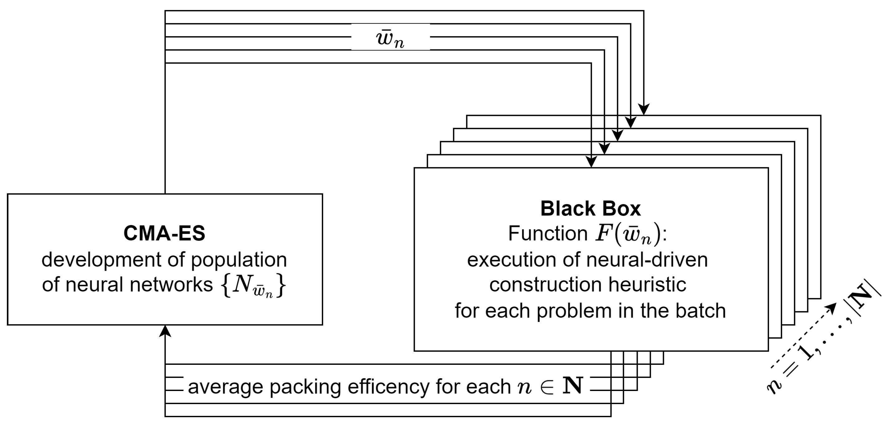
The training procedure is illustrated in Figure 7. CMA-ES, as an evolutionary strategy algorithm, searches the space of neural network weights and optimizes a given function F. The algorithm operates iteratively on a population $\mathbf{N}$, where each individual $n\in \mathbf{N}$ represents a distinct set of neural network weights ${\overline{w}}_n$, and thus a unique neural network $N_{{\overline{w}}_n}$. To control the evolution of the population, CMA-ES evaluates every individual $n\in \mathbf{N}$ in the population. To mitigate the computational burden associated with evaluating all training instances, we adopt a batch-based approach, using only a subset of instances per iteration. Specifically, for each CMA-ES iteration, 100 problem instances are randomly drawn from a pool of 500,000. Thus, the population is evaluated against a newly sampled subset of instances at each cycle.

Evaluation of an individual $n\in \mathbf{N}$ involves executing the algorithm depicted in Figure 5 with the individual’s weights ${\overline{w}}_n$ on each problem in the batch. As illustrated in Figure 7, weights ${\overline{w}}_n$ are passed to the black-box evaluation in parallel for each $n\in \mathbf{N}$. This process results in a set of packings for each n, corresponding to the batch of problems.

For each packing, the packing efficiency factor is computed based on the number of closed bins and the fill factor of the last (potentially partially filled) bin. The average packing efficiency over all problems in the batch serves as the quality metric for the corresponding individual, effectively acting as a fitness function.

From the perspective of CMA-ES, the evaluation of an individual n is perceived as a black-box function, as no explicit information about the function structure is available. The average packing efficiencies are collected for all individuals, and CMA-ES uses this information to guide the evolution of the population, generating the next generation of individuals.

This random selection of a modest subset per iteration effectively alters the objective function throughout the optimization process. Nevertheless, the algorithm sustains convergence while keeping computational demands manageable. Additionally, this unconventional strategy reduces the risk of the algorithm becoming trapped in local optima.

Notably, unlike many other optimization methods [50], CMA-ES relies on the relative ranking of evaluation outcomes rather than their precise numerical values. This means that the optimization is driven by the performance order of individuals rather than their specific scores, enhancing the algorithm’s robustness and supporting convergence even when the objective function fluctuates during training.

Every 10th iteration, the best solution found in that iteration is evaluated against a predefined validation set of 10,000 problems. The best-performing solution on the validation set so far is stored as the final solution of the algorithm.

4. Computational Experiments

4.1. Baseline Solution

As the proposed neural-driven heuristic aims to replace traditional rule-based item selection and placement strategies with neural-based decision-making, we compare it against well-established single-pass algorithms: MaxRects and Skyline [21]. The main principle of operation of both algorithms requires sorting the items then placing each item in a selected bin and positioning it within the bin.

For item sorting, we consider both natural order (non-sorted list) and descending order based on the following attributes:

• item area,
• item perimeter,
• absolute difference in side lengths,
• shorter side length,
• longer side length,
• ratio of side lengths.

For placement selection, we tested all standard criteria for MaxRects and Skyline, yielding ten heuristics as described in [21]:

• MaxRects-Based Heuristics:

  −

  Maximal Rectangles Bottom-Left (MaxRectsBl),

  −

  Maximal Rectangles Best Area Fit (MaxRectsBaf),

  −

  Maximal Rectangles Best Short Side Fit (MaxRectsBssf),

  −

  Maximal Rectangles Best Long Side Fit (MaxRectsBlsf),

• Skyline-Based Heuristics:

  −

  Skyline Bottom-Left (SkylineBl),

  −

  Skyline Bottom-Left Wast Map Improvement (SkylineBlWm),

  −

  Skyline Min Waste Fit (SkylineMwf),

  −

  Skyline Min Waste Fit with low profile (SkylineMwfl),

  −

  Skyline Min Waste Fit with Waste Map Improvement (SkylineMwfWm),

  −

  Skyline Min Waste Fit with low profile and with Waste Map Improvement (SkylineMwflWm).

Based on results presented in [21], for bin selection, we adopt the best performing heuristic, the Bin Best Fit (BBF) rule, where an item is placed in the bin that yields the best score according to the selected placement heuristic.

Additionally, we test a global approach (as described in [21]) where items are not pre-sorted. Instead, the placement score determines both the bin selection and the next item to place. In this strategy, we evaluate placement scores across all bins and choose the best combination of item and placement position. For instance, in the MaxRects-BSSF variant, the selected item and position minimize the shorter leftover side, defined as ${min}_{(f,i)}\left(min(w_f-w_i,h_f-h_i)\right)$, where $(w_f,h_f)$ denote the width and height of free space f, and $(w_i,h_i)$ represent the width and height of item i.

As a baseline, we select the best result obtained from all MaxRects and Skyline heuristic combinations for each problem type and size. This serves as an oracle-based benchmark, assuming an ideal scenario where the best heuristic is known in advance for each dataset.

4.2. Datasets

We employed two distinct approaches to generate test problem instances. The first leverages the 2DCPackGen problem generator, designed for two-dimensional rectangular cutting and packing problems [12]. The second simulates real-world logistic scenarios, incorporating predefined bin dimensions and a constrained set of item sizes. Throughout this paper, we refer to datasets generated by these methods as 2DCPackGen and logistic datasets, respectively.

For both problem generation methods and each problem type and size, we generated a total of 510,000 training instances, divided as follows:

• 500,000 instances used exclusively for training the neural network.
• 10,000 instances reserved for validation, used to evaluate and select the best-performing neural network across training iterations.

To ensure a fair comparison between the neural-driven heuristic and the benchmark heuristics (MaxRects and Skyline), we generated an additional 10,000 instances for each combination of problem type and size. These instances were generated using a different random seed to keep them distinct from the training problems, and they were solely used for performance evaluation.

4.2.1. Datasets Generated with 2DCPackGen

Following the typology of Wäscher et al. [1], we generated problem instances of the Single Stock Size Cutting Stock Problem (SSSCSP) type using algorithms implemented in 2DCPackGen. Each problem instance is defined by the tuple $(L_1,W_1,l_t,w_t,d_t^l)$, where $L_1$ and $W_1$ represent the length and width of the bin, respectively, $t\in T$ denotes an item type from the set of types T, and $l_t$, $w_t$, and $d_t^l$ indicate the length, width, and quantity of items of type t, respectively.

The 2DCPackGen generator accepts a variety of parameters, with those pertinent to the weakly heterogeneous single stock size CSP problem type listed in

Table 4. Parameters of the 2DCPackGen problem generator.

#	Parameter Name	Value (Min…Max)
1	Number of dimensions:	2
2	Integer seed:	10,000
3	Number of instances:	510,000
4	Bin’s size dimensions:	1000…1000
5	Items’ size dimensions:	100…500
6	ID of the size and shape characteristic of items:	1, 6, 2 or 16
7	Number of different item types:	5, 10 or 15
8	Item type demand:	1…10 or 1…20
9	Distribution of item type demand:	uniform

. These parameters, stored in a dedicated parameter file utilized by 2DCPackGen, govern the characteristics of the generated instances.

We set the bin dimensions to $W=H=1000$ (parameter #4). Problem instances include three different numbers of item types: 5, 10, and 15 (parameter #7).

The dimensions of each item type ($w_t$,$l_t$) were randomly generated as integer values within the range $[100,500]$ (parameter #5). Item sizes and shapes followed one of four predefined characteristics:

• Small and square (ID = 1),
• Big and square (ID = 6),
• Long and narrow (ID = 2),
• Mixed sizes, i.e., a combination of small and square, short and tall, long and narrow, and big and square (ID = 16),

where ID refers to the generator’s identifier for the items’ size and shape characteristics (parameter #6).

For each item type, the number of items was randomly drawn from a uniform distribution (parameter #9), using either range [1, 10] or [1, 20] (parameter #8). We apply a uniform distribution due to the lack of prior knowledge regarding the specific distribution of items. Furthermore, adopting a different distribution would imply incorporating additional domain-specific knowledge, thereby potentially simplifying the problem. The use of a uniform distribution is also common practice in the literature, as evidenced by several studies (e.g., [51,52]).

When selecting parameters for the 2DCPackGen generator, our primary goal was to ensure diversity among the generated problem instances. In summary, we evaluated problem instances with varying numbers of item types (parameter #7), different ranges for item type demand generation (parameter #8), and diverse size and shape characteristics of the generated item types (parameter #6).

Table 5. Statistics of 2DCPackGen problem instances.

Num. of Item Types	Item Type Demand	Avg. Num. of Items	Heterogeneity Measure
	1–5	15.0	0.33
5	1–10	27.5	0.18
	1–20	52.5	0.09
	1–5	30.0	0.33
10	1–10	55.0	0.18
	1–20	105.0	0.09
	1–5	45.0	0.33
15	1–10	82.5	0.18
	1–20	157.5	0.09

presents key statistics for these instances, including the average number of items and a heterogeneity measure, defined as the ratio of the number of item types to the average number of items per instance.

4.2.2. Real-Life Logistic Datasets

In practical pallet-based packing, item sizes are typically standardized—e.g., trays of yogurt, packs of water, or canned goods often share consistent dimensions across manufacturers. These sizes are generally designed to align with standard pallet dimensions, such as the Euro pallet (1200 × 800 mm), enabling efficient space utilization. Ideally, a single layer of identical items should maximize pallet coverage, which is readily achieved through patterned arrangements. A grid pattern is particularly effective, requiring item dimensions to be divisors of the pallet’s dimensions. While alternative patterns are feasible, they are less commonly observed in practice.

Based on real-world item dimensions used in the fast-moving consumer goods (FMCG) industry, we created a predefined set of item sizes, categorized as large, medium, and small items.

Table 6. Item dimensions (mm) for the real-life logistic problems.

Small	Medium	Large
(100, 100)	(171, 100)	(266, 109)
(109, 100)	(171, 114)	(266, 120)
(114, 100)	(171, 133)	(266, 133)
(114, 109)	(171, 160)	(266, 150)
(120, 100)	(200, 100)	(266, 171)
(120, 114)	(200, 109)	(266, 200)
(133, 100)	(200, 114)	(266, 240)
(133, 109)	(200, 120)	(300, 133)
(133, 114)	(200, 133)	(300, 160)
(133, 120)	(200, 150)	(300, 200)
(133, 133)	(200, 160)	(300, 240)
(150, 100)	(200, 171)	(300, 266)
(150, 114)	(200, 200)	(400, 160)
(150, 133)	(240, 100)	(400, 171)
(160, 100)	(240, 114)	(400, 200)
(160, 109)	(240, 133)	(400, 240)
(160, 120)	(240, 160)	(400, 266)
(160, 133)	(240, 200)	(400, 300)
(160, 150)	(250, 200)	(400, 400)
		(600, 266)
		(600, 400)

lists the item dimensions used in our experiments. With the exception of (300, 240) and (250, 200), all dimensions allow for a grid-based layer formation on a standard Euro 1 pallet. The two exceptional cases also permit single-layer packing but require a different pattern.

We classified items on their larger dimension, using the following size ranges:

• Small: 100–160 mm
• Medium: 171–250 mm
• Large: 266–600 mm

Additionally, we introduced a fourth category (Mixed), which includes all Small, Medium, and Large item sizes.

As previously, we generated problems with a predefined number n of distinct item types: 5, 10, and 15. The demand for each item type was drawn as a uniformly random integer from the ranges [1, 10] or [1, 20].

To create random test instances for a given category of item dimensions, number of item types, and demand range, we first sampled n unique dimensions from the category. Then, for each dimension, we assigned a demand as a uniformly distributed random integer within the specified range. The bin consistently corresponds to a standard Euro pallet with dimensions 1200 × 800 mm.

4.3. The Results

The algorithm was implemented in C++. For black-box optimization, we utilized the CMA-ES library from the Laboratory for Computer Science, Université Paris-Sud (https://github.com/CMA-ES/libcmaes, accessed on 3 February 2025), authored by Emmanuel Benazera and supported by Nikolaus Hansen, a co-author of the original method. The neural network has been implemented from scratch, leveraging Eigen, a C++ template library for linear algebra (http://eigen.tuxfamily.org, accessed on 3 February 2025). Unless otherwise mentioned, all experiments were conducted on a PC-class computer equipped with a 12-core processor, operating at an average clock speed of 4.3 GHz.

Based on our preliminary tests, we configured the population size to 384 and the initial step-size parameter $\sigma$ to 0.4. The optimization terminates after 500,000 black-box function evaluations, equivalent to approximately 1300 iterations. We employed the Sep-CMA-ES variant, which achieves linear computational complexity with respect to the number of dimensions by restricting the covariance matrix to a diagonal form [53].

To compare the proposed neural-driven heuristic with benchmark heuristics, we adopted the number of bins required to pack all items as the primary objective, which is always an integer number. This differs from the objective used during the training of the neural-driven heuristic, which combines the number of closed bins with the fill factor of the last, potentially partially filled bin.

Table 7. 2DCPackGen datasets: Number of cases (out of 10,000) where the neural-driven heuristic outperformed (underperformed) benchmarking heuristics.

Item Types	Item Type Demand	Size and Shape ID
		1		6		2		16
5	1–10	946	(18)	1832	(85)	1533	(47)	707	(86)
	1–20	1716	(18)	3300	(111)	2964	(58)	1358	(126)
10	1–10	1737	(2)	4212	(65)	3210	(9)	1713	(68)
	1–20	3718	(0)	6334	(103)	6127	(5)	3045	(102)
15	1–10	2487	(3)	5945	(51)	4587	(0)	2812	(60)
	1–20	5163	(0)	7839	(79)	8590	(1)	4756	(57)

and Figure 8 summarize the results for 2DCPackGen datasets. The neural-driven heuristic outperforms the oracle (constructed from benchmark heuristics) across all cases. The proportion of instances where our algorithm is strictly superior ranges from 7% (for 5 item types, demand range [1, 10], and mixed sizes denoted by ID = 16) to 86% (for 15 item types, demand range [1, 20], and long, narrow items denoted by ID = 2). Instances where our algorithm underperforms are rare, typically below 1%, with a maximum of 1.26% for mixed sizes with few item types. Notably, performance improvements increase with higher numbers of item types and greater demand ranges, highlighting the neural-driven approach’s advantage on more complex datasets.

For further insight,

Table 8. 2DCPackGen datasets: Average (over 10,000 test problems) number of bins computed by the neural-driven construction heuristic and benchmarking heuristics (in parentheses).

Item Types	Item Type Demand	Size and Shape ID
		1		6		2		16
5	1–10	1.9	(2.0)	5.8	(6.0)	3.0	(3.2)	3.2	(3.3)
	1–20	3.1	(3.2)	10.7	(11.0)	5.3	(5.6)	5.7	(5.8)
10	1–10	3.2	(3.3)	10.9	(11.4)	5.4	(5.7)	5.8	(6.0)
	1–20	5.5	(5.9)	20.4	(21.2)	9.8	(10.5)	10.6	(10.9)
15	1–10	4.5	(4.7)	16.0	(16.6)	7.8	(8.2)	8.4	(8.7)
	1–20	8.0	(8.5)	30.0	(31.2)	14.3	(15.3)	15.5	(16.0)

reports the average number of bins required across problem classes, as computed by the neural-driven heuristic and benchmark heuristics. Our approach consistently achieves a lower average bin count in all cases.

Figure 9 shows a selected example of packings obtained by the neural-based heuristic and the benchmarking heuristics. This is a typical case where our approach uses one less bin while the benchmarking heuristics struggle to pack small items due to the lack of space in the first bins. Our method generates less waste in the first two bins and can pack small items of type 0 and 3.

Table 9. Logistic datasets: Number of cases (out of 10,000) where the neural-driven heuristic outperformed (underperformed) benchmarking heuristics.

Item Types	Item Type Demand	Dimensions Category
		Small		Medium		Large		Mixed
5	1–10	0	(1)	949	(3)	1353	(37)	686	(22)
	1–20	642	(11)	1057	(12)	2388	(10)	1125	(11)
10	1–10	1278	(3)	1225	(0)	1823	(5)	1074	(2)
	1–20	949	(3)	2194	(0)	3111	(1)	1976	(2)
15	1–10	164	(0)	1634	(0)	2085	(1)	1497	(1)
	1–20	1379	(0)	3140	(0)	3826	(0)	2735	(0)

and Figure 10 present results for logistic datasets. Similar to the 2DCPackGen datasets, our neural-driven heuristic surpasses the oracle of benchmark heuristics in all cases. However, due to the higher regularity of item sizes relative to bin dimensions, the improvement is slightly less pronounced. The percentage of improved cases increases with more item types and higher demand, peaking at over 38% for 15 item types, demand range [1, 20], and large items. Unlike the 2DCPackGen datasets, the mixed category does not consistently exhibit the lowest improvement; instead, small items typically show the least gain. Although improvements are smaller than those for 2DCPackGen datasets, the proportion of worse cases is also lower, rarely exceeding 0.05%. An exception occurs with small items, 5 item types, and demand range [1, 10], where all items typically fit into one bin. We retained these results for consistency across problem sizes.

Table 10. Logistic datasets: Average (over 10,000 test problems) number of bins computed by the neural-driven construction heuristic and benchmarking heuristics (in parentheses).

Item Types	Item Type Demand	Dimensions Category
		Small		Medium		Large		Mixed
5	1–10	1.0	(1.0)	1.3	(1.4)	2.9	(3.0)	1.7	(1.8)
	1–20	1.3	(1.4)	2.1	(2.2)	5.0	(5.2)	2.9	(3.0)
10	1–10	1.3	(1.4)	2.2	(2.3)	5.2	(5.4)	3.0	(3.1)
	1–20	2.2	(2.3)	3.8	(4.0)	9.4	(9.7)	5.3	(5.5)
15	1–10	2.0	(2.0)	3.1	(3.2)	7.5	(7.7)	4.3	(4.4)
	1–20	3.1	(3.2)	5.4	(5.7)	13.8	(14.2)	7.7	(8.0)

reports the average number of bins for logistic datasets. The neural-driven heuristic achieves a lower or equal average bin count in all cases, with equality occurring only for small items with five item types and demand range [1, 10].

Figure 11 illustrates an exemplary packing achieved by the neural-based heuristic and the baseline algorithm. As it may be noticed, most of the items can be arranged in a way that covers a whole or almost whole bin with very little waste. However, it requires dynamic changes in the rules while packing, and thus, such packing is not delivered by any of the benchmarking heuristics. That results in a need to use a fourth bin, which is poorly filled-in.

Table 11. 2DCPackGen datasets: average time (over 10,000 test problems) to solve one problem with neural-driven heuristic [ms].

Item Types	Item Type Demand	Size and Shape ID
		1	6	2	16
5	1–10	0.18	0.09	0.12	0.11
	1–20	0.32	0.17	0.23	0.18
10	1–10	0.56	0.30	0.44	0.4
	1–20	1.27	0.68	0.84	0.72
15	1–10	1.27	0.74	0.97	0.68
	1–20	2.65	1.23	1.89	1.42

and

Table 12. Logistic datasets: average time (over 10,000 test problems) to solve one problem with neural-driven heuristic [ms].

Item Types	Item Type Demand	Dimensions Category
		Small	Medium	Large	Mixed
5	1–10	0.19	0.18	0.12	0.14
	1–20	0.27	0.23	0.20	0.23
10	1–10	0.58	0.55	0.36	0.45
	1–20	1.06	0.87	0.69	0.88
15	1–10	1.18	1.02	0.75	1.02
	1–20	2.33	1.94	1.44	1.73

present the average computation times for the two datasets obtained when the algorithm was run only on one core. Differences between the two datasets are not pronounced. For the 2DCPackGen dataset, computation times are highest for size and shape ID 1, corresponding to scenarios with many small items, and lowest for ID 6, which represents larger, square items. This trend is expected, as a greater number of small items increases the number of iterations required by the constructive algorithm. A similar pattern is observed in the logistic dataset, where computation times are higher for small items and decrease for medium and large items. Regarding item type demand, computation times approximately double (typically slightly less than a factor of 2), consistent with the maximal demand, which is also doubled. In both datasets, the number of item types has the most significant impact on computation time: more item types require greater computational effort. Overall, computation times range from 0.18 to 2.65 ms, which is notably short, particularly when compared to the typical computation times of conventional metaheuristics. For instance, recent papers report computational times ranging from 2 s to 1700 s for a genetic algorithm [54], and approximately 1 to 7 s for Variable Neighborhood Search, Simulated Annealing, Ant Colony Optimization, and Particle Swarm Optimization algorithms [55].

5. Conclusions

In this paper, we introduced a novel neural-driven constructive heuristic for the two-dimensional cutting stock problem (2D-CSP) or, equivalently, the bin packing problem with weakly homogenous items. We consider the variant of the problem that involves so-called robotic packing, which ensures the feasibility of packing with robots.

The key strength of this approach lies in its ability to leverage problem-specific characteristics to score candidate placements dynamically. Unlike traditional heuristics, which rigidly follow predefined rules based on single properties or very small property vectors, our method employs a broader property vector that notably includes information about the current packing state. Consequently, the learned heuristic has the potential to adapt to the current state, enabling more responsive and context-aware decision-making during the packing process.

A critical component of the proposed heuristic is the design of features that describe the current partial solution, enabling an effective evaluation of candidate placements. These features go beyond simple measures like item count and area utilization. Instead, they incorporate structural properties that help capture pattern formation potential, such as horizontal and vertical size-fit properties.

Unlike most existing methods, which rely on reinforcement learning or deep learning to generate placements, our approach employs a neural network exclusively as a scoring mechanism for candidate decisions. This ensures full independence from the problem’s dimensional complexity, avoiding the challenge of a variable input size, which typically complicates neural network design and training. Moreover, our method leverages compact, straight-forward neural networks, allowing us to optimize them efficiently using population-based black-box optimization instead of traditional backpropagation. This also eliminates the issue of intermediate reward assignment in reinforcement learning, as network evaluation is based solely on the final packing performance.

Experimental results highlight the superiority of our method over the oracle-based approach, with improvements observed in up to 86% of cases across the 2DCPackGen datasets. Notably, the most significant gains occur in more complex instances, characterized by greater diversity in item types and higher item counts. These findings underscore the robustness of our heuristic in tackling challenging 2D-CSP scenarios.

We consider a wide range of item configurations, including small versus large items, square versus elongated items, and combinations of these variants. Similarly, we address problem instances featuring both a small and a large number of item types. Moreover, we incorporate logistics datasets that reflect practical scenarios observed in the fast-moving consumer goods industry. Given that the proposed approach achieves good performance across these diverse settings, it appears to be both flexible and largely robust with respect to dataset characteristics.

The proposed approach effectively addresses the algorithm selection problem in the context of state-of-the-art 2D-CSP heuristics, offering a flexible framework with the potential for broader generalization. Future work could explore its adaptability to other optimization problems, particularly those for which constructive heuristics already exist. These include, for instance, the Job Shop Scheduling Problem, the Traveling Salesman Problem, and the Strip Packing Problem, among others. Additionally, incorporating further features to enhance performance or to address specific problem variants—such as priority-based bin packing—represents a promising research direction. Finally, integrating a local search component into the heuristic could enable better solution fine-tuning, albeit at the cost of increased computational effort, and facilitate benchmarking against metaheuristic methods.