Abstract
This study addresses the performance degradation of and - filters in 6G Integrated Sensing and Communications (ISAC) scenarios, attributed to violations of linearity and steady-state assumptions. These filters are originally designed with time-invariant gains derived under such assumptions to ensure low computational complexity. However, deviations from ideal conditions—such as non-white, biased, or non-Gaussian process noise—necessitate corrective mechanisms. We propose a weighted process noise approach that accounts for increased uncertainty due to assumption violations while preserving the filters’ closed-form structure and computational efficiency. By integrating uncertainty into the conventional gain formulation, the proposed method achieves performance closer to the optimal filter. Numerical results demonstrate superior accuracy over conventional filters across various noise variances and scenarios, without requiring parameter tuning. Notably, performance improvements become more pronounced as the measurement interval decreases.
1. Introduction
Integrated Sensing and Communications (ISAC) have been identified as a key enabler for 6G networks, driving the convergence of communication and sensing functionalities within a unified framework. Among the core enablers of ISAC, state estimation technologies—such as object tracking and localization—are becoming increasingly critical for a wide range of applications, including autonomous systems, smart environments, and wireless network optimization. In this context, Kalman filtering remains a fundamental and powerful approach for state estimation, particularly due to its recursive structure and suitability for real-time implementation. As ISAC systems demand higher precision, robustness, and computational efficiency, research on the practical design, adaptation, and implementation of Kalman filters is gaining renewed importance [1,2].
The Kalman filter is derived under the assumptions that the system dynamics and measurement models are linear, and that both the process noise and measurement noise are zero-mean, white, and Gaussian. Additionally, the process and measurement noises are assumed to be mutually independent, with known and stationary covariances [3]. Based on these assumptions, the Kalman filter has become a widely used algorithm in target tracking and has inspired various extensions such as the steady-state Kalman filter, Extended Kalman filter, Unscented Kalman filter, and Particle filter [4]. Among these, we focus on improving the tracking performance of the Kalata model, a simplified version of the Kalman filter derived under steady-state assumptions to reduce computational complexity. The Kalata model achieves time-invariant gain by assuming steady-state conditions, but its performance often degrades in real-world scenarios where these assumptions are violated. Such limitations can lead to higher errors than measured values or reduced noise suppression capability. However, on the computational side, the Kalata model acquires predefined gains and then repeatedly applies these values during the real-time estimation process. Conversely, time-variant gain filters, such as the Kalman filter, Extended Kalman filter, and Particle filter, require repetitive gain calculations and additional computations at each step.
The filter is a one-dimensional approach that estimates the current position by combining predicted and measured values using a gain parameter, . This method can be considered a low-pass filter. The - filter extends the filter by incorporating velocity estimation through an additional gain parameter, , as initially proposed by Benedict and Bordner [5]. In this model, is expressed as a function of , which is typically determined via simulation. To address the computational inefficiency of simulations, Kalata introduced a closed-form solution for using the tracking index, a parameter that relates maneuverability uncertainty to measurement uncertainty [6,7]. In addition, several studies have explored models using damping parameters [8,9] and MV filters [10]. These models exhibit various relationships and differences, as discussed in [9,11,12,13]. This study aims to improve the relationship between the tracking index and the gain of the Kalata model, which is based on the steady-state Kalman filter. To enhance the Kalata model, research has also been conducted on estimating position, velocity, and acceleration using position and velocity measurements [14,15]. For a brief comparison of these models, refer to Table 1. The -- filter, a straightforward extension of the - filter, is excluded from this discussion for simplicity.

Table 1.
Brief comparison with model of coefficient tracking filter.
While the Kalata model provides computational efficiency by assuming steady-state conditions, it faces significant challenges in real-world applications. These include increased errors in non-linear systems, degraded performance during convergence periods, and sensitivity to poorly designed system matrices or noise parameters. Such limitations highlight the need for improved models that can handle process noise uncertainties and deviations from steady-state assumptions. In particular, defining optimal values for the gain parameters such as and is crucial to enhancing the Kalata model’s performance. These parameters directly influence the filter’s ability to balance noise suppression and responsiveness to dynamic changes. Without well-defined and values, the model’s effectiveness can significantly deteriorate under varying conditions. Therefore, improving the relationship between the tracking index and these gain parameters is essential for achieving robust and efficient tracking in practical applications.
In this study, we propose an enhanced and - filter framework that incorporates weighted process noise uncertainty into the Kalata model. By redefining the relationship between the tracking index and filter gains such as and , our approach adjusts the Kalman gain to account for non-Gaussian process noise and real-world uncertainties [16]. To address these issues, the proposed method considers the uncertainty caused by deviations from steady-state assumptions by weighting the process noise to better reflect its influence on system performance [17]. This approach eliminates reliance on simulations or tuning processes while maintaining computational simplicity. Our findings demonstrate improved robust tracking performance in non-ideal ISAC environments where traditional steady-state assumptions fail, while preserving closed-form simplicity.
The rest of this paper is organized as follows. The overall system model and and - filter system models are introduced in Section 2. The existing and - filters based on the Kalman filter, called the Kalata model, and the limitations of the steady-state-based model are introduced in Section 3. The proposed weighted process noise method is introduced in Section 4. The analysis of the proposed method is compared with the Kalata model in Section 5. The performance analysis is presented in Section 6. Our main conclusion is described in Section 7.
2. System Model
Assume that the position is received as a measurement. The system and measurement equations are then given as follows:
where, is the state vector at time k that we want to know, and A is the state matrix that connects the previous and current state. represents the maneuver/state transition matrix to include the acceleration state. is the measurement at time k that includes measurement noise, and H is the domain matrix that represents the relationship between the state and the measurement. and denote process noise and measurement noise, respectively.
The Kalman filter operates in two main steps: the prediction step, which estimates the current state and its uncertainty based on the previous estimate and system model, and the update step, which refines this prediction by incorporating new measurement information. The steady-state Kalman filter equations are expressed as follows:
- 1.
- Prediction:
- 2.
- Update:
2.1. Filter Model
The filter is designed such that the dimensions of the target state vector match those of the measurement and the estimation domain .
The parameters of the mathematical model and Kalman gain are defined as follows:
where T denotes the time interval. Accordingly, the state and measurement equations can be written as
The estimation and prediction equations are expressed as follows:
- 1.
- Prediction:
- 2.
- Estimation:
2.2. - Filter Model
The - filter is an extension of the filter that uses measured position data to estimate two target state vectors: position and velocity. This approach reduces the prediction error covariance when predicting the position. The state vector for this model is defined as
where represents the position and represents the velocity at time k. The parameters of the mathematical model and Kalman gain are defined as follows:
where is the position gain and is the velocity gain. The system and measurement equations can be expressed as
The estimation and prediction equations are expressed as follows:
- 1.
- Prediction:
- 2.
- Estimation:
3. Preliminaries on Kalata Model
3.1. Design of and - Filters Based on the Kalata Model
The Kalata model was first proposed by P.R. Kalata as a closed-form, steady-state simplification of the full Kalman filter, motivated by the need to reduce the per-step computational load in radar tracking applications while retaining near-optimal performance when its underlying assumptions are satisfied. Steady-state refers to a condition where the system’s behavior stabilizes over time, such that key parameters no longer vary with time. Under this assumption, the Kalman gain becomes time-invariant, simplifying computations while maintaining effective performance in stable environments. The tracking index, denoted as , is defined as the ratio of process noise to measurement noise
and it quantifies the ratio of process noise uncertainty to measurement noise uncertainty over one sampling interval. A larger indicates higher target maneuverability relative to sensor noise, which drives the choice of time-invariant gains and .
For the filter, the Kalata model defines the gain parameter as
This equation ensures that is optimized for steady-state conditions, balancing noise suppression and responsiveness. The tracking performance of the filter is expressed as
where represents the estimation error variance for position. This shows that tracking performance improves as increases, reducing the impact of measurement noise.
For the - filter, both position gain and velocity gain are derived based on the tracking index, . The relationship between and is given by
In this context, the value of plays a critical role in determining the filter’s behavior. When , the filter prioritizes smoothing velocity estimates, reducing fluctuations caused by noise. This is particularly useful in scenarios where stability and noise suppression are more important than rapid responsiveness. Conversely, when , the filter enhances prediction accuracy by responding more aggressively to changes in the target’s motion. This makes it suitable for highly dynamic environments where quick adaptation to maneuverability is required. The tracking performance of the - filter can be evaluated using the following equations:
where represents the estimation error covariance for position and velocity, and represents the estimation error variance for velocity. While the Kalata model simplifies implementation by assuming steady-state conditions , it has limitations in dynamic or non-linear environments where steady-state assumptions may not hold. In such cases, deviations from steady-state conditions can lead to increased prediction errors or reduced noise suppression capabilities. Enhancing tracking performance requires incorporating process noise uncertainty into the model design to ensure robust operation in real-world applications.
3.2. Limitation of Steady-State Model
The Kalata model, as described in Section 3.1, is derived based on the steady-state Kalman filter. This approach offers a significant advantage by providing a time-invariant gain, which reduces computational effort by eliminating the need to compute the Kalman gain at each step. However, these benefits come with several limitations that can impact performance in real-world applications:
- Non-linear systems: the steady-state assumption leads to a time-invariant gain, which may cause divergence or suboptimal performance in non-linear systems where dynamic changes occur frequently.
- Convergence period: even if the system eventually reaches a steady state, performance degradation can occur during the convergence period. This delay can be critical in scenarios requiring rapid adaptation to changes in target motion.
- Sensitivity to system design: the model’s performance is highly sensitive to poorly designed system matrices, including process noise covariance, measurement noise covariance, and the state transition matrix. Errors in these parameters can lead to significant inaccuracies.
- Real-world constraints: the steady-state assumption inherently relies on ideal conditions, such as white, zero-mean, and uncorrelated process noise. In real-world environments, these assumptions are often violated due to external factors and system uncertainties, leading to reduced smoothing performance or higher errors compared with measured values.
These limitations highlight the challenges of applying the steady-state Kalman filter or Kalata model directly to real-world systems. For instance, when process noise deviates from Gaussian characteristics or when the system operates under dynamic conditions that break steady-state assumptions, the model’s effectiveness diminishes significantly. To address these issues, it is essential to incorporate methods that account for process noise uncertainty and deviations from steady-state conditions via weighted process noise. By doing so, tracking performance can be improved, even in environments where traditional steady-state models fail to deliver optimal results.
4. Designing and - Filters with Consideration of Process Noise Uncertainty
The Kalata model’s and - filters offer a significant advantage in terms of computational efficiency compared with the traditional Kalman filter. The Kalata model is derived from the steady-state Kalman filter, which assumes a time-invariant gain. Under ideal conditions—where the system is linear and the process noise is white Gaussian noise—the Kalman filter achieves optimal mean square error performance. However, in real-world applications, the steady-state assumption is often violated. This leads to process noise properties that deviate from being uncorrelated and zero-mean. Furthermore, maintaining the Gaussian distribution of process noise becomes challenging when comparing theoretical assumptions with real-world scenarios. These deviations result in a failure to adequately reflect the uncertainty of the process noise distribution. In our work, we address this limitation by designing filters that account for weighted process noise that does not follow a Gaussian distribution. Our approach incorporates the uncertainty of non-Gaussian process noise into the filter framework, ensuring more robust performance in dynamic and uncertain environments.
A Gaussian Mixture Model (GMM) is a probabilistic model that assumes that all the data points are generated from a mixture of a finite number of Gaussian distributions with unknown parameters. The GMM is mathematically defined as
where K represents the number of Gaussian components, and are the mixing coefficients, satisfying and . Each denotes the k-th Gaussian component with mean and covariance matrix . The GMM is also referred to as a “weighted linear combination of Gaussian component densities” and is considered a universal approximator [18]. This means that, with a sufficient number of Gaussian components, the GMM can approximate any continuous probability distribution. The entropy of a Gaussian distribution is defined as follows:
The entropy of a Gaussian distribution is directly proportional to its variance. As such, the entropy of a GMM is also proportional to its variance. Among all probability distributions defined over the real line with the same finite mean and variance, the Gaussian distribution has the maximum entropy. Consequently, for distributions with identical variance, the entropy of a Gaussian distribution is greater than that of a non-Gaussian distribution. This property allows us to address cases where the uncertainty of the process noise distribution is not adequately reflected by introducing weighted process noise. For background information, see [19].
If the uncertainty of process noise, caused by the limitations of the system model, is identified and reflected, the Kalman gain can be appropriately adjusted to account for this uncertainty. However, accurately considering such uncertainty requires either a deep understanding of the real system or the use of numerical methods to estimate it. The Kalman gain is fundamentally determined by the reliability of measurement noise and prediction error. When the prediction model is well-designed, it places greater emphasis on predictions; conversely, when the model is relatively inaccurate, it relies more on measurement values. The steady-state assumption in the Kalman filter presumes that process noise is white, zero-mean, and uncorrelated. However, this assumption does not account for increased uncertainty when process noise deviates from these characteristics due to system model limitations. In real-world scenarios, it is particularly challenging to maintain these assumptions. To address this issue, we redefine the formula for the tracking index by incorporating innovation covariance and prediction error covariance. This redefinition reflects the uncertainty caused by process noise that does not adhere to the steady-state assumptions.
Equation (40) represents the innovation, which is the difference between the actual measurement and the predicted measurement. Equation (42) represents the innovation covariance, which measures the uncertainty in the innovation and has the same domain as the measurement domain. If we transform it to have the same domain as the state vector, we can derive Equation (43) through Equation (41). The innovation is critical to the Kalman filter, as it quantifies the discrepancy between observed data and model predictions. The innovation covariance reflects how much uncertainty exists in this discrepancy and is key in determining the Kalman gain. It can be expressed as follows:
By transforming the innovation covariance to align with the state vector’s domain, we ensure consistency in how uncertainties are represented across different domains. This transformation allows for a more accurate update of the state estimate, especially when dealing with systems where measurement noise and prediction errors vary significantly. Equation (45) modifies the Kalman gain to account for the measurement-to-measurement domain. Equation (47) reflects the relative reliability of the prediction error covariance and the innovation covariance, specifically within the domain directly associated with the measurements. This adjustment ensures that the Kalman gain appropriately balances the influence of prediction accuracy and measurement reliability. By decomposing Equation (47), we can further analyze its components to understand how it reflects three critical characteristics
The above formula reflects three main characteristics as follows:
- The balance between measurement and smoothed predictions.
- The balance between measurement and smoothed measurements.
- The relationship between measurement and process covariance.
These characteristics emphasize how the inverse of the modified Kalman gain integrates process noise uncertainty into its design, thereby facilitating more robust performance in dynamic and uncertain environments.
Thus, the inverse of the modified Kalman gain is adjusted to reflect the relative influence of the prediction error covariance and the measurement noise covariance, alongside the process covariance. To extend this approach to the process noise domain, we transform the modified gain from the measurement domain to the state vector’s domain. By applying this transformation through the relationship, it can be expressed as follows:
Thus, is directly affected by process noise in the same domain as the measurement. As mentioned before, when the assumption is violated, we adjust the relationship between prediction and measurement through gain in the update phase. can be interpreted as a practical scaling parameter that quantifies the additional process noise uncertainty arising from modeling errors or non-Gaussian disturbances not captured by the idealized system model and adjusts the influence of process noise in the filter’s update accordingly. Thus, serves as a means of balancing responsiveness to new data and noise suppression, enabling the filter to maintain reliable performance even when the underlying assumptions of linearity or steady-state are violated. However, the uncertainty in measurement noise, which is often assumed to be uncorrelated and stationary, can lead to performance degradation when not properly accounted for in the gain transformation. The of the filter and - filter is as follows:
In Equations (52) and (53), represents the gain, which is directly linked to the measurement domain. In Equation (53), the placement of the matrix form is chosen to exactly match the measurement domain. This alignment ensures that the gain is correctly scaled to the uncertainties inherent in the measurement process. In other words, the filter’s response to measurement uncertainty is preserved because the gain operates within the same context as the measurement data. As a result, this formulation guarantees that any adjustments made due to changes in the measurement noise or process noise are accurately reflected in the computed Kalman gain. By directly associating the gain with the measurement domain, the filter can more effectively balance the weight between prediction and observation. This, in turn, enables the filter to adapt its performance under non-ideal conditions where the process noise may not strictly conform to the white, zero-mean, uncorrelated assumptions. Consequently, our modified filter formulation improves its robustness and tracking accuracy by ensuring that the uncertainties across both the measurement and prediction domains are consistently and appropriately managed.
Figure 1 illustrates the algorithm diagram for the filter and the - filter. In these filters, the Kalman gain is predefined as it is time-invariant under steady-state assumptions. In our work, the relationship equation of the tracking index is redefined to incorporate the uncertainty of process noise into the calculation of the Kalman gain. As a result, the gain represented by is treated as a constant, equivalent to the Kalman gain, and only influences the tracking index relationship equation. In other words, while this modification does not directly impact the performance relationship equation, it does lead to numerical changes in and , which subsequently affect tracking performance. The system and measurement equations are proposed as follows:
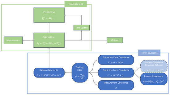
Figure 1.
Estimation algorithm of and - filters.
For the filter, the parameters are defined as follows:
Thus, it can be expressed as follows:
The estimation and prediction equations remain consistent with Equations (15) and (16). The prediction error covariance and estimation error covariance are defined as
Using Equations (61) and (62), a new definition of the tracking index relationship for can be established
For the - filter, the parameters are defined as
The corresponding system equations are
The estimation and prediction equations remain consistent with Equations (23) and (24). The prediction error covariance and estimation error covariance are defined as
Using Equations (67) and (68), a new definition of the tracking index relationship for and can be established. The relationship between the tracking index and gain is as follows:
In this formulation, is redefined as
For smoothing purposes, remains between 0 and 1, consistent with the Kalata model. However, in our proposed model, also falls between 0 and 1, unlike in the original Kalata model where could range from 0 to 2.
5. Analysis of Designing and - Filters with Consideration of Process Noise Uncertainty
Figure 2 illustrates the relationship between the tracking index and the gain parameter, . The proposed and - filters exhibit higher values of compared with the Kalata model’s filters for the same tracking index. This indicates that, under the proposed framework, greater reliance is placed on measurement values when the prediction model does not perform well using previously estimated values. Consequently, the proposed filters prioritize measurement data more heavily than the Kalata model.
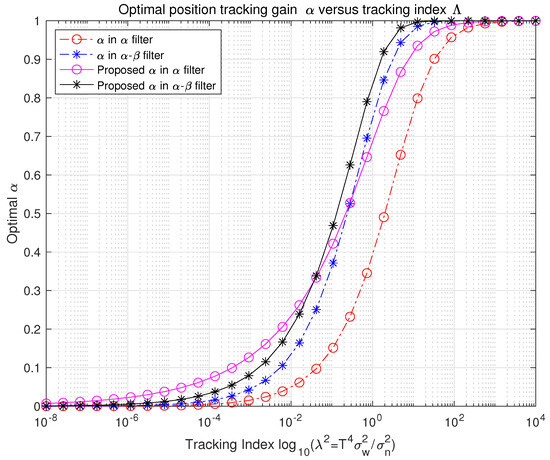
Figure 2.
Alpha−tracking index relationship.
Figure 3 shows the behavior of in the proposed - filter. When the tracking index is relatively low, the value of is slightly higher compared with the Kalata model’s - filter. This adjustment reflects lower process noise in the ratio of process noise to measurement noise. Conversely, as the tracking index increases, the value of in the proposed filter becomes lower than that in the Kalata model. This reflects higher process noise in the ratio, accounting for increased uncertainty in process noise.
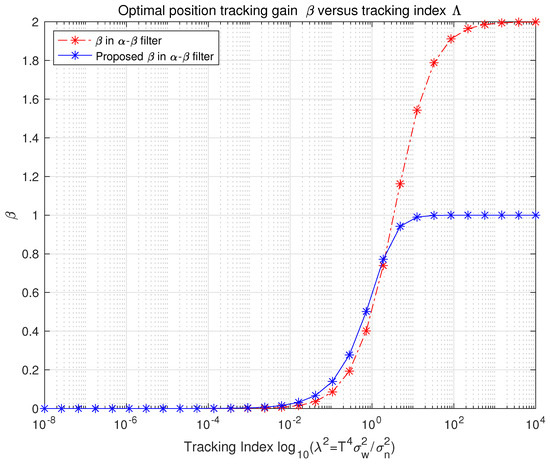
Figure 3.
Alpha−beta−tracking index relationship.
Higher values of and make the filter more responsive to new measurements, allowing it to quickly adapt to rapid changes or maneuvers in the target’s motion. However, this increased sensitivity can also make the filter more susceptible to measurement noise, resulting in less smoothing of the estimates. Conversely, lower values of and cause the filter to rely more on the prediction from the system model, which leads to smoother estimates and better noise suppression. However, this comes at the cost of slower adaptation to sudden changes or maneuvers in the target’s motion, and may also lead to degraded performance when there is a mismatch between the idealized model assumptions and the actual system dynamics.
Table 2 summarizes key differences between the Kalata model’s filters and the proposed filters. The proposed filters redefine the relationship between the tracking index and gain parameters (, ), resulting in improved robustness against non-Gaussian process noise and deviations from steady-state assumptions. The proposed filters, like the traditional Kalata model, define and in advance using closed-form equations, so the computational complexity during real-time operation remains the same. Any additional complexity from calculating these parameters offline is negligible.
Table 2.
Comparison of tracking index relationship and gain parameters in and - filters.
6. Performance Analysis
The performance analysis of the proposed and - filters was conducted through simulations under three different scenarios: exponential, sine, and steady-state functions (Figure 4, Figure 5 and Figure 6). The purpose of this analysis was to evaluate the effectiveness of the proposed filters in dynamic environments compared with the Kalata model’s filters. The shape of the simulation function under the condition is as follows:
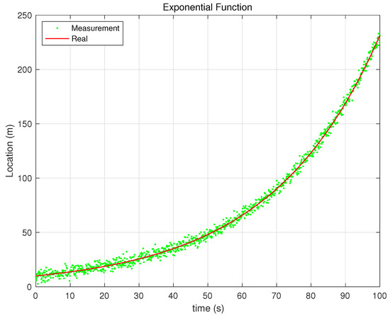
Figure 4.
Exponential Function.
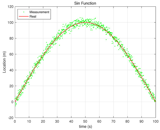
Figure 5.
Sin Function.
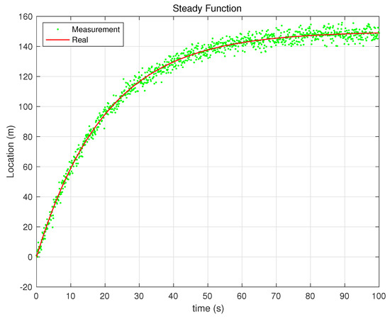
Figure 6.
Steady Function.
In simulation, the parameters are as follows:
- Time interval: 0.1 s;
- Operation time: 100 s;
- Iteration: .
Process noise and measurement noise are as follows:
The process noise in Table 3 is obtained through Equations (13) and (20), and the measurement noise has a variance of [0.001, 0.01, 0.1, 1, 10, 100] with additive white Gaussian noise. The performance of each filter is evaluated based on the errors observed in position estimations.
Table 3.
Process noise according to environment and filter frameworks.
In the simulation, the table and graph of errors are as follows:
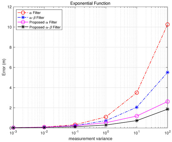 Figure 7. Exponential Function error.
Table 4. Exponential Function error.
Figure 7. Exponential Function error.
Table 4. Exponential Function error.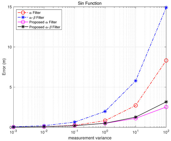 Figure 8. Sin Function error.
Table 5. Sin Function error.
Figure 8. Sin Function error.
Table 5. Sin Function error.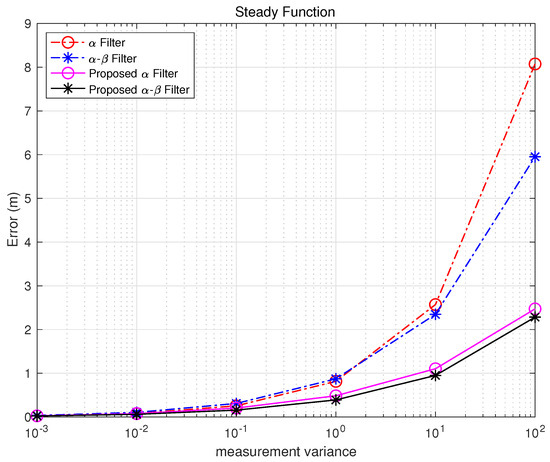 Figure 9. Steady Function error.
Table 6. Steady Function error.
Figure 9. Steady Function error.
Table 6. Steady Function error.
In some cases of rapid or highly non-linear changes, the filter can outperform the - filter, as shown in Figure 8. This indicates that both conventional and proposed filters with time-invariant gains have limitations in fully utilizing additional state information during abrupt dynamics.
In the case of the steady-state function, if the maintenance time after convergence approaches , the performance of the Kalata model improves significantly. This is because, during the steady-state period, the time-invariant gain of the Kalata model ensures consistent and precise tracking under stable conditions. However, if the focus shifts to tracking performance during periods of high maneuverability, rather than precision during the maintenance period after convergence, the proposed and - filters demonstrate superior performance.
Figure 10, Figure 11, Figure 12, Figure 13 and Figure 14 illustrate how each filter performs in different scenarios when the measurement noise variance is set to 10. The proposed filters consistently outperform their Kalata counterparts in dynamic environments, particularly during rapid changes in motion. This highlights their ability to adaptively adjust gain parameters to reflect process noise uncertainty.
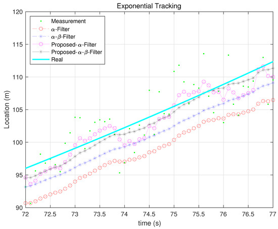
Figure 10.
Exponential Function tracking.
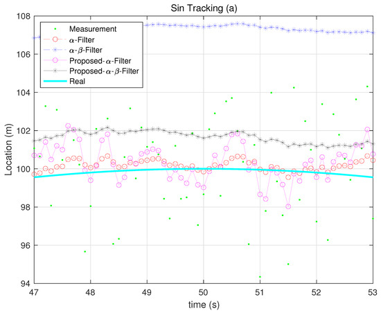
Figure 11.
Sin Function tracking 1.
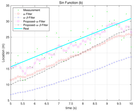
Figure 12.
Sin Function tracking 2.
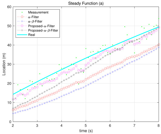
Figure 13.
Steady Function tracking 1.
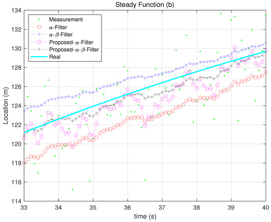
Figure 14.
Steady Function tracking 2.
Figure 15, Figure 16 and Figure 17 represent the ratio of estimation to measurement for each function based on the time interval. Using the inverse variance weighting method, the measurement standard deviation was divided by the estimation error of each measurement noise for every time interval, and the results were summed.
is the ratio of estimation/measurement for the i-th time interval, and is the estimation error of the j-th measurement noise in the i-th time interval. This ratio provides a quantitative assessment of estimator performance. Specifically:
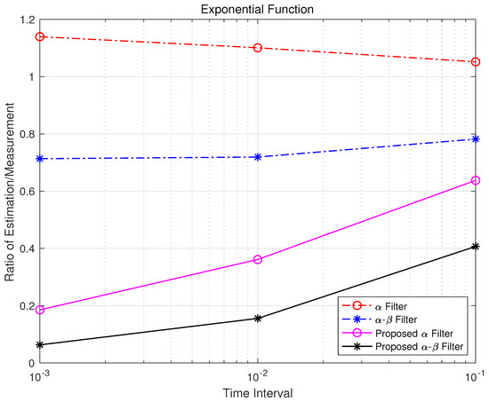
Figure 15.
Exp error time interval.
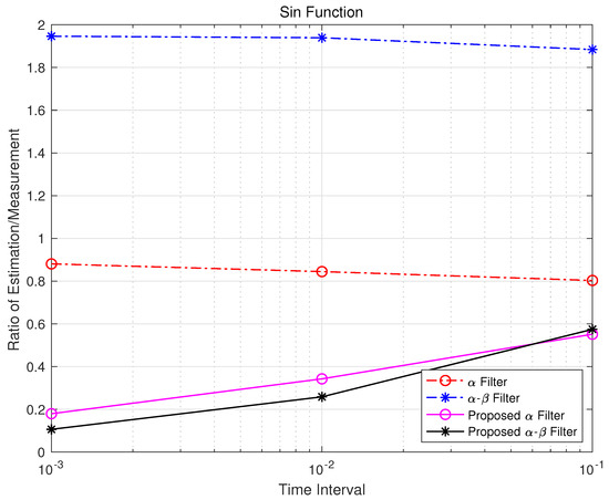
Figure 16.
Sin error time interval.
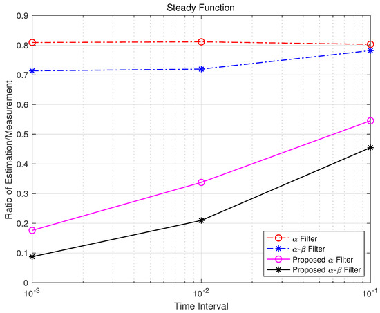
Figure 17.
Steady error time interval.
- If exceeds 1, it indicates that the estimation error is greater than the measurement value, signifying poor estimator performance.
- If is less than 1, it shows effective estimation, with values closer to zero reflecting higher accuracy.
The analysis reveals that, as the time interval decreases, the proposed and - filters exhibit significant improvements in mitigating non-linear effects. This demonstrates their robustness and adaptability in dynamic environments compared with traditional steady-state models.
7. Conclusions
In this paper, we propose enhanced and - filters by establishing a new relationship between the tracking index and filter gains to mitigate performance degradation observed in 6G ISAC scenarios. This degradation stems from violated assumptions of linearity and steady-state conditions, which are common in real-world environments. Specifically, we were motivated by the observation that non-Gaussian process noise—resulting from such violations—exhibits lower entropy than Gaussian noise with the same variance, indicating a mismatch between assumed and actual system uncertainty. To address this, we introduced a weighted process noise model that accounts for this uncertainty while maintaining the closed-form solution and computational complexity of the conventional filters. This modification impacts the measurement update step, enabling the filter to better adapt to model inaccuracies without sacrificing efficiency. Numerical simulations demonstrated that the proposed filters consistently outperformed the conventional Kalata model’s and - filters across a wide range of scenarios and noise conditions. In particular, the proposed method showed strong tracking performance under high maneuverability, which is a critical consideration in ISAC systems. Additionally, when the measurement time interval decreased, the proposed filters exhibited further performance gains in mitigating the effects of noise, highlighting their robustness in high-update-rate environments. Importantly, the proposed filters required no tuning or additional simulations, underscoring their practicality for real-world deployment. Nonetheless, the increased gain introduced by our approach may result in reduced smoothing, especially in applications where stability is prioritized over responsiveness. As future work, the proposed framework may be extended to incorporate time-varying gain designs or be further optimized for specific application domains such as embedded systems, signal processing, and localization. Such advancements would contribute toward realizing the goals of 6G ISAC by providing low complexity yet adaptive state estimation solutions.
Author Contributions
Conceptualization, J.-B.K. and S.-W.C.; methodology, J.-B.K. and S.-W.C.; software, J.-B.K.; validation, J.-B.K. and S.-W.C.; formal analysis, J.-B.K. and S.-W.C.; investigation, J.-B.K.; resources, J.-B.K.; data curation, J.-B.K.; writing—original draft preparation, J.-B.K.; writing—review and editing, S.-W.C.; visualization, J.-B.K.; supervision, S.-W.C.; project administration, J.-B.K. and S.-W.C.; funding acquisition, S.-W.C. All authors have read and agreed to the published version of the manuscript.
Funding
This work was supported by the Institute of Information & communications Technology Planning & Evaluation (IITP) grant funded by the Korea government (MSIT) (No. 2021-0-00165, Development of 5G+ Intelligent Base Station Software Modem).
Data Availability Statement
The original contributions presented in this study are included in the article. Further inquiries can be directed to the corresponding author.
Conflicts of Interest
The authors declare no conflict of interest.
Abbreviations
| GMM | Gaussian Mixture Model |
| ISAC | Integrated Sensing and Communications |
References
- Kaushik, A.; Singh, R.; Dayarathna, S.; Senanayake, R.; Renzo, M.D.; Dajer, M.; Ji, H.; Kim, Y.; Sciancalepore, V.; Zappone, A.; et al. Toward Integrated Sensing and Communications for 6G: Key Enabling Technologies, Standardization, and Challenges. IEEE Commun. Stand. Mag. 2024, 8, 52–59. [Google Scholar] [CrossRef]
- Wang, J.; Varshney, N.; Gentile, C.; Blandino, S.; Chuang, J.; Golmie, N. Integrated Sensing and Communication: Enabling Techniques, Applications, Tools and Data Sets, Standardization, and Future Directions. IEEE Internet Things J. 2022, 9, 23416–23440. [Google Scholar] [CrossRef] [PubMed]
- Faragher, R. Understanding the basis of the Kalman filter via a simple and intuitive derivation. IEEE Signal Process. Mag. 2012, 29, 128–132. [Google Scholar] [CrossRef]
- Simon, D. Optimal State Estimation; John Wiley & Sons: Hoboken, NJ, USA, 2006. [Google Scholar]
- Benedict, T.R.; Bordner, G.W. Synthesis of an optimal set of radar track-while-scan smoothing equations. IEEE Trans. Autom. Control 1962, 7, 27–32. [Google Scholar] [CrossRef]
- Kalata, P.R. The tracking index: A generalized parameter for α-β and α-β-γ target trackers. IEEE Trans. Aerosp. Electron. Syst. 1984, AES-20, 174–182. [Google Scholar] [CrossRef]
- Kalata, P.R.; Chmielewski, T.A. Smoothing improvement ratio for α-β and α-β-γ tracking systems. In Proceedings of the 1992 American Control Conference, Chicago, IL, USA, 24–26 June 1992; pp. 862–866. [Google Scholar]
- Murray, W.J.; Gray, J.E. Target tracking with explicit control of filter lag. In Proceedings of the 29th Southeastern Symposium on System Theory, Cookeville, TN, USA, 9–11 March 1997; pp. 81–85. [Google Scholar]
- Gray, J.E.; Murray, W.J. A derivation of an analytic expression for the tracking index for the alpha-beta-gamma filter. IEEE Trans. Aerosp. Electron. Syst. 1993, 29, 1064–1065. [Google Scholar] [CrossRef]
- Saho, K. Design of accurate α-β tracker based on steady-state performance index. Int. J. Signal Process. Anal. 2016, 1, 001. [Google Scholar]
- Gray, J.E.; Smith-Carroll, A.S.; Murray, W.J. What do filter coefficient relationships mean? In Proceedings of the 36th Southeastern Symposium on System Theory, Atlanta, GA, USA, 14–16 March 2004; pp. 36–40. [Google Scholar]
- Jeong, T.; Njonjo, A.W.; Pan, B.F. A study on the performance comparison of three optimal Alpha-Beta-Gamma filters and Alpha-Beta-Gamma-Eta filter for a high dynamic target. TransNav 2017, 11, 55–61. [Google Scholar] [CrossRef][Green Version]
- Smith-Carroll, A.S.; Gray, J.E. General Solution to Constant Gain Tracking Filters; Report No. NSWCDD/TR-01/68; Naval Surface Warfare Center Dahlgren Division: Dahlgren, VA, USA, 2001. [Google Scholar]
- Saho, K. Fundamental properties and optimal gains of a steady-state velocity measured α-β tracking filter. Adv. Remote Sens. 2014, 3, 61–76. [Google Scholar] [CrossRef]
- Saho, K.; Masugi, M. Performance analysis of α-β-γ tracking filters using position and velocity measurements. EURASIP J. Adv. Signal Process. 2015, 2015, 35. [Google Scholar] [CrossRef]
- Ekstrand, B. Some aspects on filter design for target tracking. J. Control Sci. Eng. 2012, 2012, 870890. [Google Scholar] [CrossRef]
- Kosanam, S.; Simon, D.J. Kalman Filtering with Uncertain Noise Covariances. In Proceedings of the IASTED International Conference on Intelligent Systems and Control (ISAC), Honolulu, HI, USA, 23–25 August 2004; pp. 375–379. [Google Scholar]
- Stergiopoulos, S. (Ed.) Advanced Signal Processing Handbook: Theory and Implementation for Radar, Sonar, and Medical Imaging Real Time Systems; CRC Press: Boca Raton, FL, USA, 2000. [Google Scholar]
- Thomas, M.T.C.A.J.; Joy, A.T. Elements of Information Theory; John Wiley & Sons: Hoboken, NJ, USA, 1999. [Google Scholar]
Disclaimer/Publisher’s Note: The statements, opinions and data contained in all publications are solely those of the individual author(s) and contributor(s) and not of MDPI and/or the editor(s). MDPI and/or the editor(s) disclaim responsibility for any injury to people or property resulting from any ideas, methods, instructions or products referred to in the content. |
© 2025 by the authors. Licensee MDPI, Basel, Switzerland. This article is an open access article distributed under the terms and conditions of the Creative Commons Attribution (CC BY) license (https://creativecommons.org/licenses/by/4.0/).