1. Introduction
MPC, also known as Receding Horizon Control (RHC), is an optimization-based control strategy that predicts system behavior over a finite horizon and applies a receding horizon approach to improve performance while effectively handling constraints and disturbances [
1]. A key advantage of MPC is its feedback-based nature, which compensates for disturbances and modeling errors, while its predictive capability allows it to anticipate future behavior, making it well suited for nonlinear systems such as autonomous vehicles [
2]. However, MPC’s computational complexity and sensitivity to model accuracy present challenges, often necessitating robust or adaptive formulations. Uncertainty affects cost functions, constraints, and system dynamics. Learning-based MPC integrates machine learning to refine predictive models, enhancing adaptation to nonlinearities and uncertainties through real-time or offline updates. Some approaches also optimize constraints and cost functions to improve closed-loop performance [
3].
This work focuses on learning system dynamics. Robust MPC ensures constraint satisfaction under uncertainty by decomposing system dynamics into a nominal model and an additive uncertainty term [
3]. Robust methods can be categorized as parametric or non-parametric. Parametric approaches confine uncertainties within feasible sets, iteratively refining them using system observations to ensure recursive feasibility and stability. Non-parametric approaches estimate system behavior directly from data without assuming a predefined uncertainty set, relying on gradient constraints to approximate the uncertain function. While effective for nonlinear systems, these methods are computationally demanding. Several robust learning techniques exist. Set Membership Estimation (SME) iteratively refines feasible parameter sets to maintain constraint satisfaction [
4], with applications in adaptive MPC for real-time parameter refinement [
5]. Robust adaptive Nonlinear Model Predictive Control (NMPC) integrates Least Squares minimization, leveraging kernel-based estimators for improved accuracy [
6]. Kinky Inference, a non-parametric method, provides deterministic error bounds in system modeling [
7]. Stochastic MPC explicitly accounts for uncertainty by incorporating probability distributions to construct confidence sets [
3].
Gaussian Process (GP) regression is widely used in stochastic learning-based MPC to model system dynamics under additive Gaussian noise [
8]. Applications include improved trajectory tracking in autonomous racing [
9,
10] and real-time adaptation in mobile robotics [
11]. Sparse GP approximations and dynamic data selection mitigate computational burdens [
12]. GP-based models also enhance path tracking under uncertainty [
13] and improve constraint handling in aggressive maneuvers [
14,
15].
Bayesian Linear Regression (BLR) is another probabilistic learning approach for adaptive control, incorporating prior knowledge and updating with new data. Weighted Bayesian Linear Regression (wBLR) enhances learning-based MPC by balancing short-term adaptation with long-term knowledge retention, outperforming Gaussian Processes in predictive accuracy and computational efficiency [
16].
Deep learning has been applied to MPC for capturing complex system dynamics. Neural networks enhance predictive accuracy through methods such as Extreme Learning Machines for error estimation [
17] and Adaptive Neuro-Fuzzy Inference Systems for improved prediction accuracy [
18]. Neural networks have been used in autonomous racing, outperforming physics-based models [
19], as well as in MPC for learning drift dynamics [
20] and improving trajectory tracking [
21].
Least Squares (LS) estimation is widely employed in adaptive MPC for real-time parameter updates. Recursive Least Squares (RLS) enables adaptive control, improving vehicle stability and trajectory tracking under varying road conditions [
22]. In autonomous racing, LS-based adaptive MPC iteratively optimizes performance [
23,
24]. Dynamic Mode Decomposition with Control (DMDc) has been applied to aircraft control, extracting linear models from data using LS regression [
25]. Auto-Regressive with Exogenous Input (ARX) models, updated through RLS, support adaptive MPC in process control and real-time hybrid simulations [
26,
27].
However, as explained in
Table 1, robust methods are often overly conservative, as they require bounding uncertainties within sets that include highly unlikely realizations. Stochastic approaches tend to be computationally intractable, particularly for nonlinear dynamics, where propagating Gaussian distributions becomes challenging. Deep learning methods, meanwhile, often lack generality and interpretability—critical properties for vehicle control.
This work focuses on implementing a sparse learning approach in a vehicle application, driven by a clear purpose. Unlike other learning methods, sparse optimization provides an interpretable and generalizable solution by approximating vehicle dynamics with a minimal set of physically meaningful functions. This approach is not only intended to enhance vehicle control but also to offer deeper insights into its true dynamics, which may be too complex to model using first-principles methods. By seeking the most accurate representation with the fewest possible functions, sparse optimization strikes a balance between precision and computational efficiency, making it a promising tool for autonomous vehicle applications, enabling online implementation. To summarize, the main objectives of this work are the following:
To investigate the effectiveness of the SINDy algorithm in identifying a parsimonious yet accurate and physically consistent vehicle dynamics model from simulation data.
To integrate the identified model within an MPC framework and assess its performance in both offline and online settings.
To evaluate the proposed approach in different scenarios, ranging from a simplified 3-degree-of-freedom (DOF) vehicle model to a high-fidelity CarMaker simulation.
2. Sparse Identification of Nonlinear Dynamics (SINDy)
The SINDy algorithm is employed in this work to derive a predictive model for NMPC. SINDy is chosen for its sparse formulation, which ensures interpretability while maintaining generality. As noted in [
28], many model discovery techniques require large datasets to accurately identify the governing dynamical equations. These methods often struggle to generalize beyond the training dataset, limiting their practical applicability. Machine learning approaches, such as neural networks, typically produce black-box models that obscure physical insights and make it difficult to enforce known constraints. In contrast, SINDy provides a framework for sparse and parsimonious modeling, enabling the identification of interpretable models even with limited data. The algorithm exploits the fact that most physical systems are governed by only a few dominant terms. By applying sparse regression techniques, SINDy extracts the most relevant terms while discarding unnecessary ones, making it both computationally efficient and interpretable. As described in [
29], to extract the dynamical equation
f of a system from the data acquired, the vector of the time history of the state
is collected and the corresponding derivative
is either measured or computed numerically. These are then arranged into two matrices, (
1) and (
2), where
n represents the state dimension and
m the number of sampling instants.
Additionally, the control vector
is defined as in (
3):
where
d represents the input dimension and
m the number of sampling instants. The input is considered to identify nonlinear functions where the system dynamics can be represented by (
4).
The library of functions
is then constructed consisting of candidate nonlinear functions given by (
5), where
represent the vectors of all product combinations of the components in
X and
U.
Each column of (
5) represents a candidate function for the dynamical Equation (
4), with only a few of these nonlinear functions being active in each row of the library function matrix. Sparse regression is used to determine the sparse vector coefficients
that indicate the nonlinear functions that will actually be used, converging to (
6).
In order to solve the sparse regression problem (
7), where
represent the
kth row of
and
the
kth row of
, two different optimization techniques can be used to identify a sparse
: LASSO or sequential threshold Least Squares.
The
term is used to sparsify the coefficient vector
, leveraging the parameter
to identify the Pareto optimal model that ensures accuracy while balancing model complexity. A broad exploration of
is conducted to determine the approximate threshold where terms are removed and the error begins to rise. SINDy has been applied in various nonlinear dynamical systems, including the Lotka–Volterra predator–prey model, the chaotic Lorenz system, the F8 Crusader aircraft model, and the HIV/immune response model [
30]. Its adaptability extends to high-dimensional systems through the use of principal components and delay coordinates, ensuring practical feasibility in real-world applications. Additionally, SINDy has been enhanced to handle constraints, noise, and outliers, making it robust for applications in fields such as adaptive flight control and rapid system identification.
A significant extension of SINDy is Constrained-SINDy, introduced in [
31], which integrates physical constraints directly into the regression process, as shown in (
8). This ensures that the identified models not only fit the data but also respect fundamental physical principles, such as energy conservation and known symmetries. By incorporating linear equality constraints, the method improves the accuracy and stability of identified equations, proving especially useful in fluid dynamics.
Another key development is Weak-SINDy (WSINDy), introduced by [
32,
33], which enhances robustness against noise and extends the algorithm’s applicability to partial differential equations. Unlike traditional methods that rely on point-wise derivative approximations, WSINDy formulates the identification problem using integral equations, minimizing noise amplification and improving numerical stability. This approach has been further refined with WENDy, introduced in [
34], which specializes in parameter estimation within known differential equation models.
SINDy-PI, proposed in [
30], addresses cases where governing equations are not easily expressible in explicit form. Traditional SINDy assumes explicit dynamical equations, but SINDy-PI allows for implicit relationships between state variables and their derivatives. This is particularly useful in applications such as fluid dynamics and systems governed by conservation laws. By systematically testing and selecting candidate terms, SINDy-PI enhances stability and noise resilience.
Recent advancements, such as SINDy-RL, introduced in [
35], integrate reinforcement learning to optimize control policies with minimal data. This approach reduces the sample complexity of reinforcement learning while maintaining interpretability. Another advancement, ADAM-SINDy, introduced in [
36], eliminates the need for predefined nonlinear terms by dynamically estimating system parameters using adaptive optimization techniques. Despite its advantages, SINDy faces challenges in handling non-smooth dynamics and missing state variables, requiring careful preprocessing, as discussed in [
35].
The integration of SINDy with MPC offers a powerful data-driven control strategy. SINDy models can be used within MPC frameworks to enhance computational efficiency while retaining essential nonlinear behaviors. Offline implementations of SINDy-MPC involve identifying a sparse model before deployment, ensuring efficient real-time control. In online applications, SINDy dynamically updates the model as new data become available, adapting the control strategy in real time.
A notable online adaptation method is Abrupt-SINDy, proposed in [
37], which rapidly updates models in response to sudden system changes. In the aerospace domain, SINDy-MPC has been applied to ducted fan aerial vehicles, as demonstrated in [
38], where the adaptive model improves trajectory tracking under uncertain conditions. Error-Triggered Adaptive SINDy (ETASI), introduced in [
39], updates the model only when prediction errors exceed a threshold, reducing computational cost while maintaining accuracy.
In aircraft dynamics, SINDyC, discussed in [
40], provides a data-efficient method for modeling unknown aerodynamic behaviors using minimal flight data. Similarly, SINDy has been applied to industrial robotics, as shown in [
41], where it enhances torque prediction and control stability in a 6-DOF industrial robot. In marine vehicle dynamics, the HLAR framework, proposed in [
42], integrates SINDy with hydrodynamic dictionary libraries to improve real-time control performance. SINDy has also been employed in soft robotics, as demonstrated in [
43], where it is combined with a Super-Twisting Sliding Mode Controller (STSMC) to achieve precise trajectory tracking.
In this work, WSINDy is not implemented due to its slower performance compared to the basic version, and noise handling is beyond the scope of this paper. Similarly, SINDy-PI is excluded as it introduces unnecessary complexity and lower efficiency in generating an effective vehicle model, as shown in the following sections. Instead, the constrained version of SINDy is used when testing on a highly realistic vehicle model to ensure physically meaningful parameters when approximating the effects of unmodeled states.
3. Control and Simulation Framework
This work proposes a learning-based MPC that leverages SINDy to develop an adaptive predictive model representing the dynamics of a vehicle. The MPC is used to control an autonomous vehicle around a track, where the predictive model is initially discovered and subsequently refined by SINDy. SINDy provides a physics-informed method to identify the vehicle dynamics, considering only terms that represent known physical functions in the related library matrix.
The following section presents and analyzes the complete framework, starting with the different scenarios involved, followed by the MPC formulation, the SINDy formulation, and finally, the overall setup. The goal of the paper is to estimate the parameters of a 3-DOF dynamic bicycle model using SINDy, with the aim of developing a fully tunable model.
3.1. Simulation Scenarios
The complete framework developed in this work is tested in different scenarios to assess its limitations and capabilities. Two different setups are developed based on their complexity, specifically in terms of the simulation vehicle model. Testing on a 3-DOF vehicle helps to evaluate the learning algorithm’s speed and its ability to accurately approximate the highly nonlinear wheel force model. The next step involves testing on a more complex and realistic vehicle model to evaluate SINDy’s performance in capturing the effects of unmodeled degrees of freedom.
It is important to note that the sparse regression approach allows for aggressive maneuvers near road limits, as demonstrated in simulations, which makes real-world validation inherently risky. Furthermore, the lack of a well-defined ground truth complicates the identification of true vehicle parameters; as a result, the analysis will be carried out exclusively in a simulation environment.
A single-track dynamic bicycle model is selected to simulate the vehicle behavior in MATLAB 2023b. As stated in [
44,
45], the dynamic bicycle model is a widely used representation to describe vehicle motion, accounting for inertial effects, yaw dynamics, and lateral tire forces. According to [
46], the following parameters are considered:
and
denote the distances from the center of mass to the front and rear wheels, respectively. The vehicle’s heading angle is represented by
, while
indicates the yaw rate. The longitudinal and lateral tire forces are denoted by
and
, respectively, where the subscripts
and
correspond to the front and rear wheels. The steering angle is represented by
, while
and
define the slip angles of the front and rear wheels, respectively. These parameters, as introduced in [
46], provide the foundation for modeling vehicle dynamics. The system’s dynamics are formulated in state-space notation as
, with the state vector
and the input vector
. These equations are expressed in a local reference frame defined by the curvilinear coordinate
s that represents the vehicle’s position along the road centerline, and the lateral deviation from the centerline
y, as in (
9). The orientation error
is defined as the difference between the vehicle’s heading angle and the tangent angle of the road centerline in the global coordinate system, given by
. The vehicle’s velocity components in the local reference frame are
,
, and
. The steering angle at the front wheels,
, and the torque applied to the rear axle,
, are obtained by integrating the inputs
and
, such that
and
. The longitudinal force
at the rear axle is equal to
divided by the wheel radius, while the lateral forces are a function of the lateral slip angles, assumed to be known and calculated following (
10). These forces are involved in describing the dynamics of the
,
, and
states and will be approximated by the SINDy algorithm.
The Magic Formula Tire Model [
47] has been employed due to its ability to provide a highly accurate mathematical representation of tire forces while accounting for nonlinear effects. This model expresses lateral force, longitudinal force, and aligning torque as nonlinear functions of slip ratio and slip angle, with
and
E serving as tuning parameters that govern the stiffness, shape, peak values, and asymmetry of the force–slip curve. In the dynamic bicycle model used in this work, only the lateral forces
and
need to be evaluated, as given in (
11):
The values used in the 3-DOF dynamic bicycle model are summarized in
Table 2, along with the parameters of the Magic Formula Tire Model.
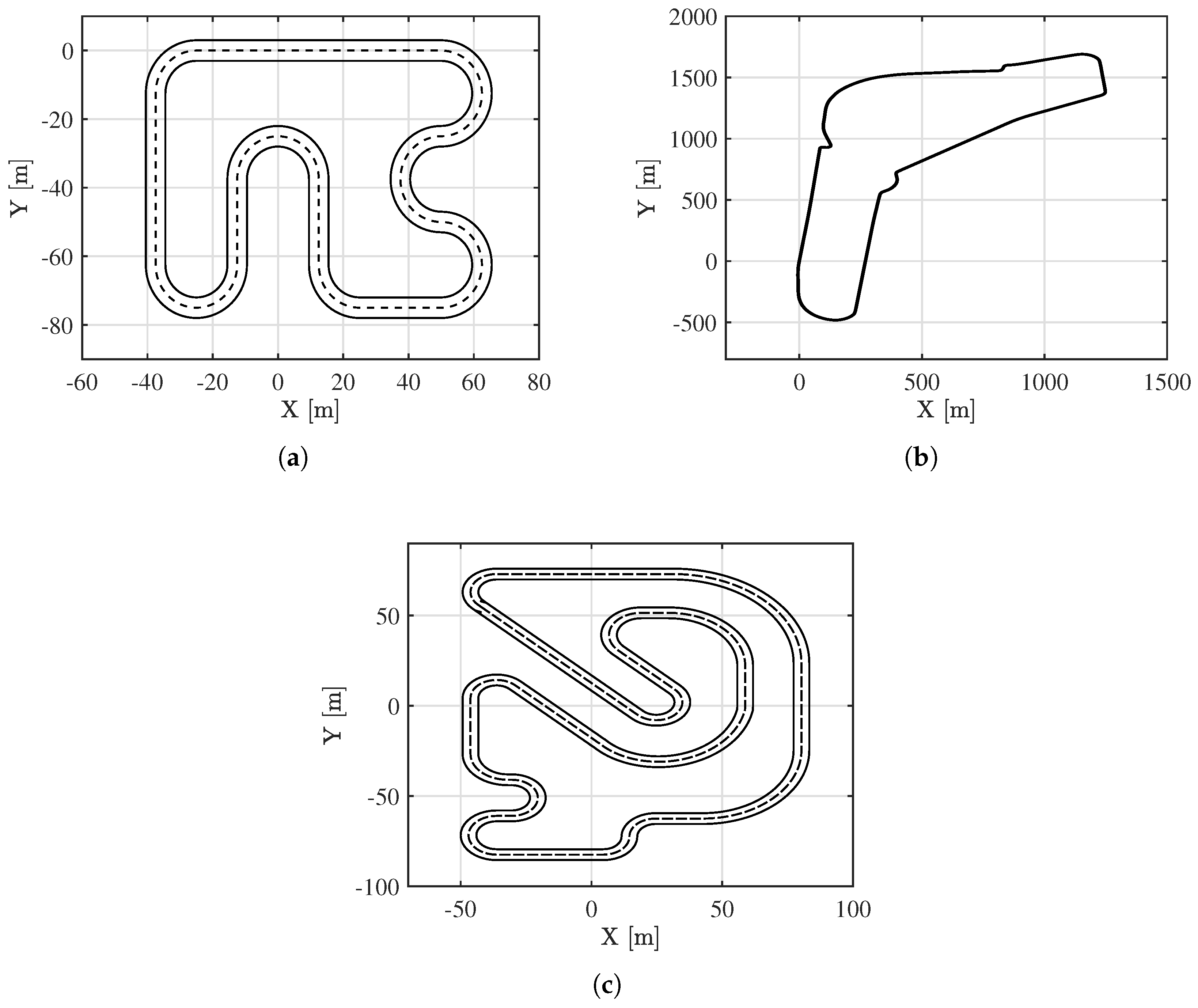
A more advanced benchmark was then developed using the CarMaker [
48] simulation software (13.1.1 version) with a high-fidelity vehicle model. The Tesla Model S in CarMaker is a detailed multibody system that accurately replicates the vehicle’s dynamics, including its electric all-wheel-drive system, regenerative braking, and advanced driver assistance features. This model enables realistic testing of autonomous driving scenarios in virtual environments. To assess the algorithm’s effectiveness, three test tracks are used, as shown in
Figure 1.
In particular, in
Figure 1 track (1a) is taken from [
49], track (1b) is the Monza Formula 1 circuit imported in CarMaker, and track (1c) is taken from [
15]. The selection of these three tracks is motivated by several factors. The first track offers a relatively simple level of complexity, allowing the algorithm to be trained on a reasonably sized dataset before being tested on more challenging circuits, such as the third one. Both tracks are also commonly used in the literature in studies relevant to this work. The Monza circuit, on the other hand, is included to provide validation within CarMaker for a highly realistic application scenario.
3.2. NonLinear Model Predictive Controller
The Nonlinear Model Predictive Controller (NMPC) used in this work is derived from [
49]. The formulated NMPC is solved using the open-source
solver [
50], where the nonlinear program (NLP) is approximately solved using the real-time iteration (RTI) scheme with a sequential quadratic programming (SQP) method.
The previously formulated vehicle dynamic model is treated as an equality constraint in the MPC formulation. In this model, the lateral tire forces are approximated by a sum of nonlinear odd functions dependent on the lateral slip angles. This approach, along with the model identified by SINDy, will be further detailed in the next section.
In the NMPC formulation, the following hard constraints are considered:
Track boundary constraint, .
Maximum steering rate, .
Maximum torque rate, .
Additionally, soft constraints are introduced to avoid discontinuities in the formulation and to ensure smoother vehicle behavior:
Track boundary constraint, .
Maximum steering angle, .
Maximum torque, .
Maximum lateral acceleration,
, constrained as follows:
Maximum longitudinal acceleration,
, constrained as follows:
To leverage efficient algorithms for solving the problem, a quadratic objective function is formulated in (
15), while the track progress of the vehicle is defined as in (
14), where
represents the vehicle’s current track progress, and
k is the step in the prediction horizon, which consists of
N steps:
where
and
represent the vehicle’s states and control inputs, respectively. The weighting matrices
are positive definite. The resulting cost function and constraints define the NLP, which is imported into
and solved using the RTI scheme within an SQP framework. The resulting quadratic programs (QPs) are then solved using the high-performance interior-point method (HPIPM).
3.3. Sparse Approximation of Vehicle Model
The core of this work is the SINDy algorithm, which not only enables the identification of a dynamic bicycle model from observed data but also provides a fully tunable model in terms of its parameters.
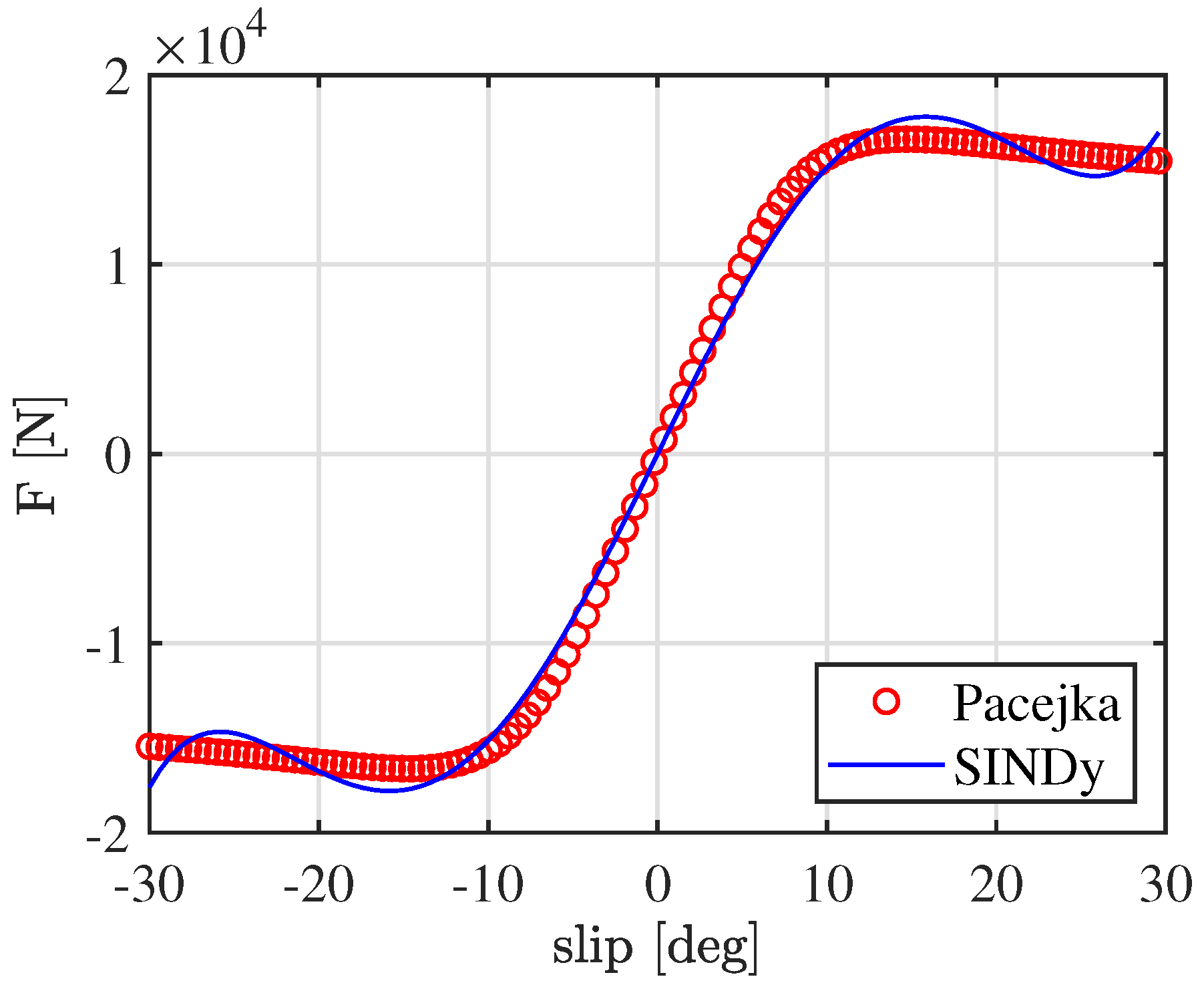
Initially, SINDy was applied offline to approximate the Pacejka tire forces as a sum of odd polynomial functions of the slip angles, which are assumed to be known (as functions of the state) and computed according to (
10). This approach is justified by the symmetry of Pacejka’s Magic Formula for lateral forces with respect to the origin, as illustrated in
Figure 2.
The approximation of Pacejka’s Magic Formula proves to be highly accurate, particularly for limited slip angle values. To preserve generality, a range of
is considered; within this range, the approximation error remains below 6%. If the slip angle range is further restricted to
, which broadly encompasses the majority of maneuvers expected from an autonomous vehicle, the error drops to approximately 1%. Subsequently, the functions to be used in the SINDy library for approximating the vehicle dynamics are selected. The objective is to transform the previously defined dynamic bicycle model in (
9) into a sum of nonlinear functions suitable for implementation in SINDy.
First, the tire force expressions are replaced with the previously identified odd polynomial functions. Then, the equations governing the dynamic behavior of the model, which define its degrees of freedom, are reformulated as a sum of functions, while the first three equations, representing the model’s geometric constraints, remain fixed. Finally, the complete model is represented in (
16), where the accelerations identified by SINDy are
,
, and
, expressed as a sum of state, input, and slip angle functions, multiplied by their associated weights
, thus resulting in a fully tunable 3-degree-of-freedom dynamic vehicle model.
In particular, recalling the SINDy general formulation in (
6), the sparse learning algorithm aims to solve the following problem (
17):
Two additional key parameters need to be properly tuned to ensure accurate model identification: the sparsity promoter parameter and the number of iterations used in the algorithm. While the number of iterations remains the same across different approaches, , the values of vary. Furthermore, normalization is particularly useful in cases where the identified weights have significantly different orders of magnitude. In such cases, the sparsity promoter parameter must be smaller than the smallest expected nonzero weight.
A constrained version of the algorithm is implemented to limit the variation of the weights discovered by SINDy in an online scenario, while attempting to approximate the effect of unmodeled states. To find the coefficients of the library functions,
solves a simple NLP consisting of the Least Squares constrained minimization problem in (
8).
The problem variables consist of the weights of the library functions, while the problem parameters include the derivative vector and the library matrix. These parameters are treated as variables because they change as the simulation progresses, incorporating newly available data. Each time the algorithm runs, these parameters update dynamically without requiring the entire problem to be recomputed. With this formulation, a computational time of around 50 ms with has been achieved. By leveraging the capacity of to generate the corresponding S-Function, the overall setup is implemented in Simulink.
Finally, the overall software in the loop (SiL) simulation setup is highlighted in
Figure 3, where the connections between the different entities used in the simulation scenario are outlined. In summary, vehicle states from CarMaker are passed to MATLAB/Simulink, where Constrained-SINDy identifies the dynamics parameters and refines the
MPC model.
MPC then generates control inputs, such as the steering angle and torque. The torque is translated into gas and brake pedal inputs, while the steering input is applied directly to the steering system. Finally, the updated inputs control the simulated Tesla Model S in CarMaker.
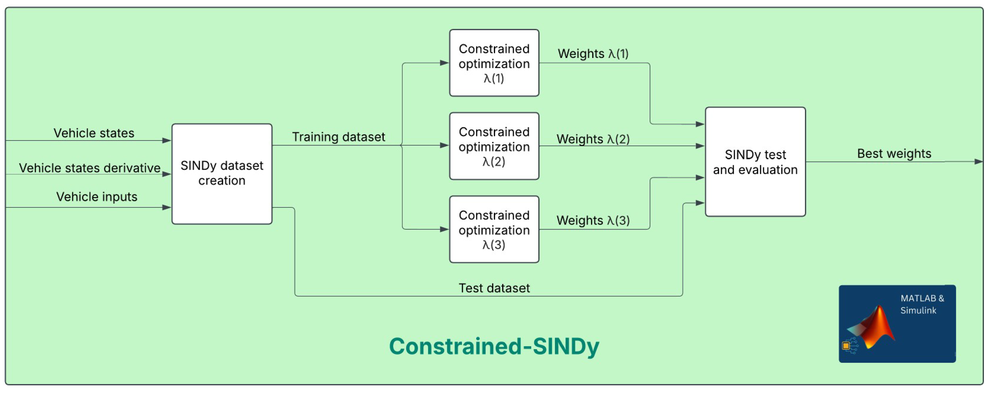
In particular, the working principle of constrained-SINDy is highlighted in
Figure 4. The machine learning algorithm aims to reconstruct the longitudinal, lateral, and yaw accelerations based on the vehicle’s inputs and states. A different sparsity-promoting parameter,
, is used for each of the three acceleration components. Once the optimal coefficients for the bicycle model are identified, they are provided as parameters to the
predictive model, which uses the same SINDy library functions. This results in a fully tunable three-degree-of-freedom vehicle model, enabling an optimized trade-off between model accuracy and simplicity.
4. Results
Initially, the tested vehicle is a 3-DOF single-track bicycle model. This same model is also used as the predictive model within the NMPC framework, with one key exception: the formulation of the tire forces. In the simulation model, the tire forces are computed using the Pacejka formulation, as described previously. However, in the predictive model, they are represented differently, as a sum of odd polynomial functions.
4.1. 3-DOF: Offline Testing
The single-track dynamic model, previously introduced and detailed in (
9), serves as the base for the simulation that operates on the track shown in
Figure 1a.
To systematically evaluate the effectiveness of the proposed algorithm, SINDy is applied to extract the weights of the functions composing the library matrix. The input to SINDy consists of both the state vector and its derivative. However, the state vector is augmented to explicitly include the lateral slip angle for both the front and rear tires. The slip angles are assumed to be available, and their values are determined using the formulation provided in (
10). The augmentation of the state vector allows SINDy to include the slip angles in the formulation of the library matrix, providing a more comprehensive representation of the system and improving the accuracy of the identified model.
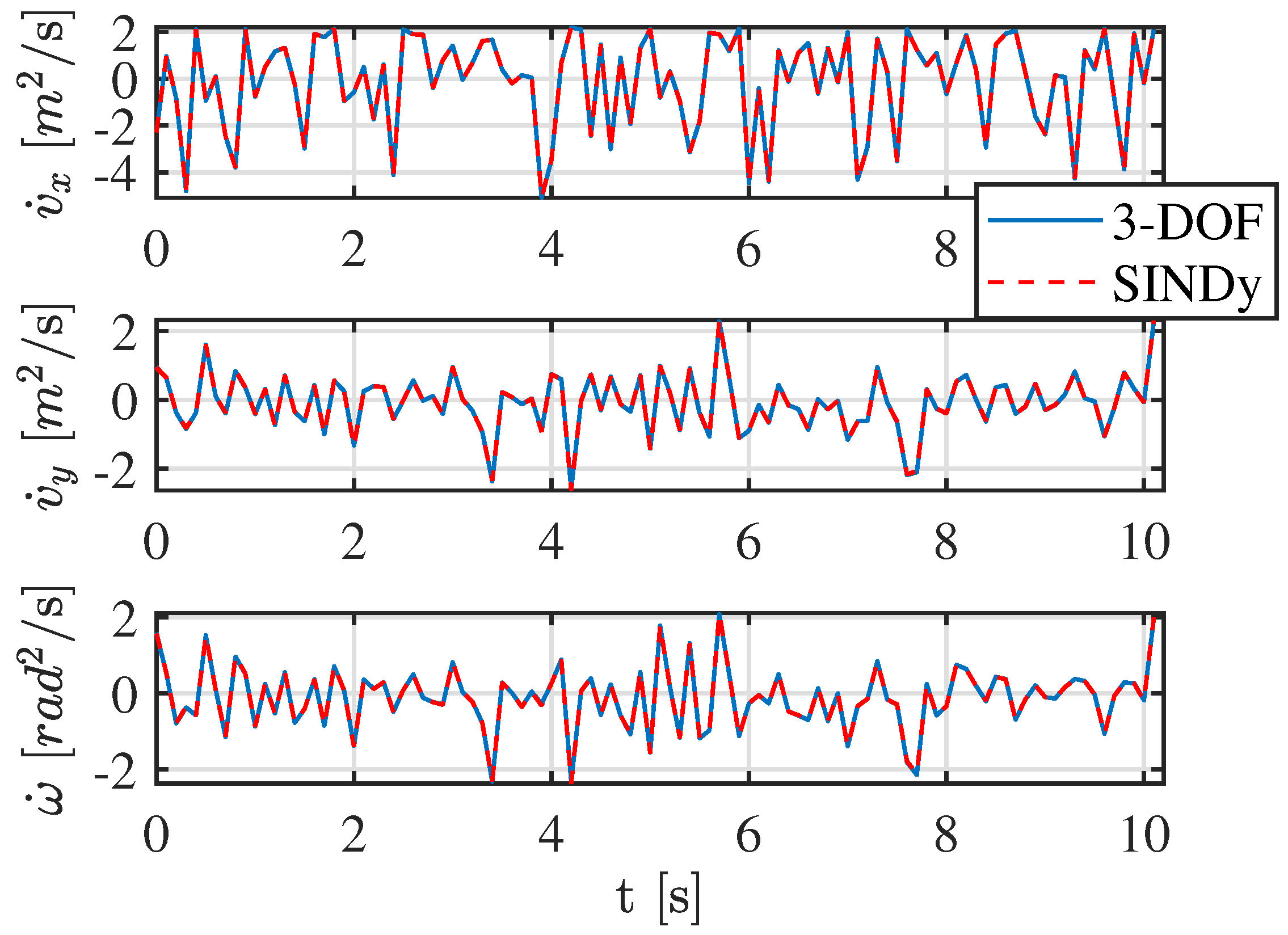
The results obtained from the application of SINDy are presented in
Figure 5 and
Figure 6. The sparse regression algorithm successfully reconstructs and approximates the simulated vehicle’s dynamics with a high degree of accuracy. As illustrated in the graph in
Figure 5, the state variables
,
, and
are effectively identified and reproduced by SINDy. This validation confirms that the learned model captures the essential characteristics of the vehicle’s dynamic behavior.
To evaluate the accuracy of the SINDy-based identification process, an error analysis is conducted using the coefficient of determination
. This metric quantifies how well the identified model captures the variance in the observed data, with values closer to 1 indicating higher accuracy. The
value is computed as in (
18), where
represents the actual system outputs,
denotes the predicted outputs, and
is the mean of the true outputs.
Figure 6 presents the
graph, constructed using the test dataset, illustrating the accuracy of the identified model in capturing the system dynamics. The high
values observed in
Figure 6 further support this, indicating that the identified equations effectively describe the system behavior. Lower values, if present, would suggest discrepancies due to model simplifications, data noise, or an insufficiently rich library of candidate functions.
Table 3 reports the percentage error of the SINDy identification along with the corresponding
values for all relevant states.
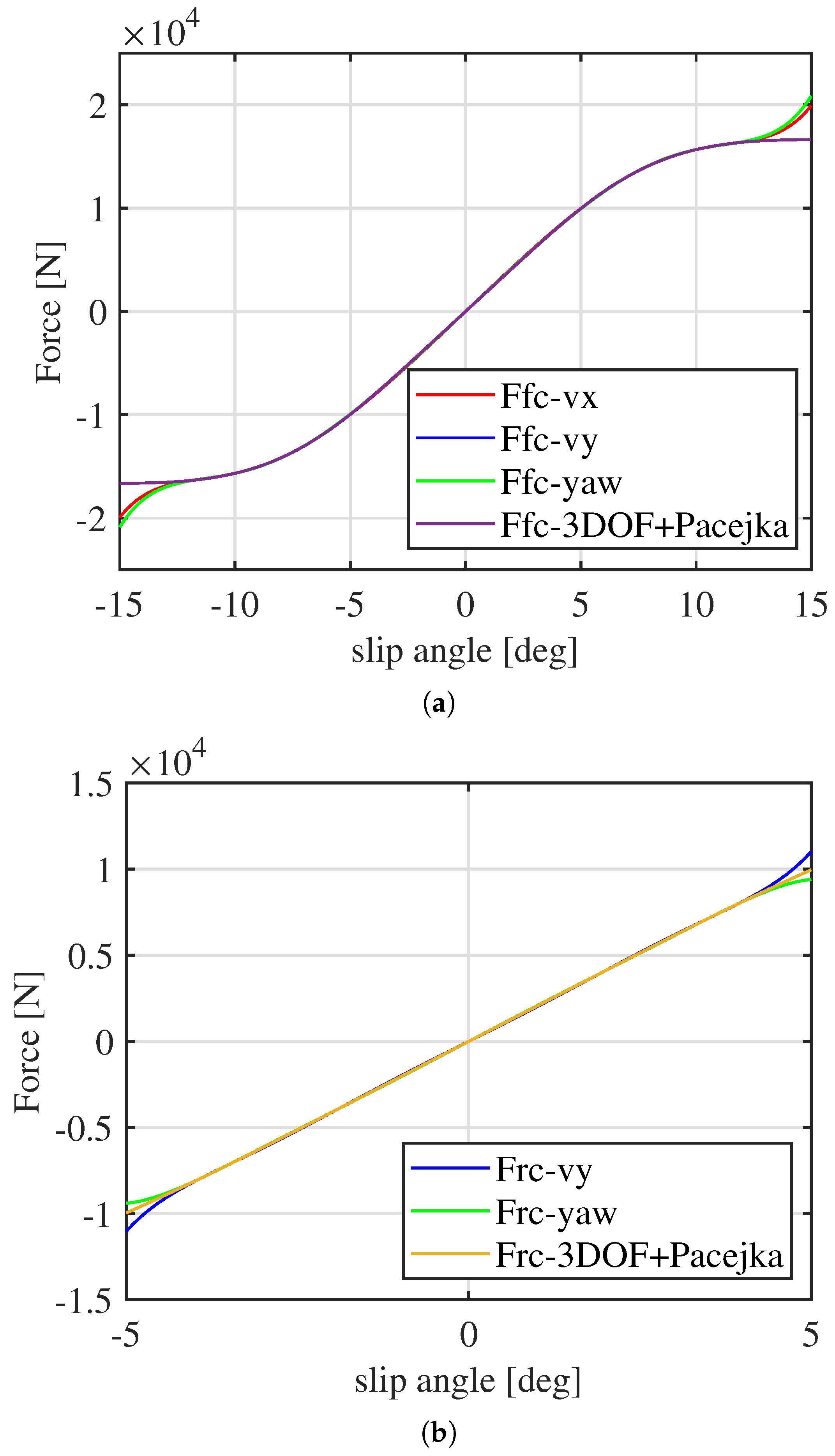
Moreover, the shape of the tire forces can also be reconstructed with the discovered weights, as shown in
Figure 7. Since the wheel forces appear in the differential equations of all three accelerations, it is possible to estimate them from each of the three equations reconstructed by SINDy. The approximation of the highly nonlinear tire forces is highly accurate within the vehicle’s operational range, demonstrating SINDy’s ability not only to estimate parameters but also to obtain a precise and fully tunable dynamic model that ensures high performance.
To further assess the generalization capability of the identified model, the simulation is performed on a different test track, shown in
Figure 1c. The choice of a distinct track is deliberate, as it allows for evaluating whether a physics-informed identification algorithm, such as SINDy, can extract a generalized vehicle model that is not overfitted to a specific training dataset. As shown in
Figure 8, the NMPC controller with the identified model successfully completes a lap on this complex track, effectively handling high slip angles.
4.2. Three Degrees of Freedom: Online Testing
At this stage, after successfully testing the offline SINDy framework on the 3-DOF vehicle, the focus shifts to evaluating its performance in an online setting. The simulation is carried out on the track shown in
Figure 1a. To investigate the real-time adaptability of SINDy, a crucial modification is introduced. Specifically, the dynamic bicycle model used in the simulation undergoes a set of parameter alterations. The parameters defining the single-track bicycle model, as well as those characterizing the Pacejka tire model, are randomly perturbed by up to 20%, in a simulation scenario similar to the one performed by [
15]. This controlled modification introduces an element of unpredictability, simulating real-world conditions where vehicle parameters might change due to variations in road conditions, tire wear, or load distribution. Before the start of the third lap, SINDy activates, allowing the algorithm to adjust the predictive model in real time. The newly computed weights capture the altered dynamics, refining the approximation of the single-track bicycle model as it responds to the evolving conditions.
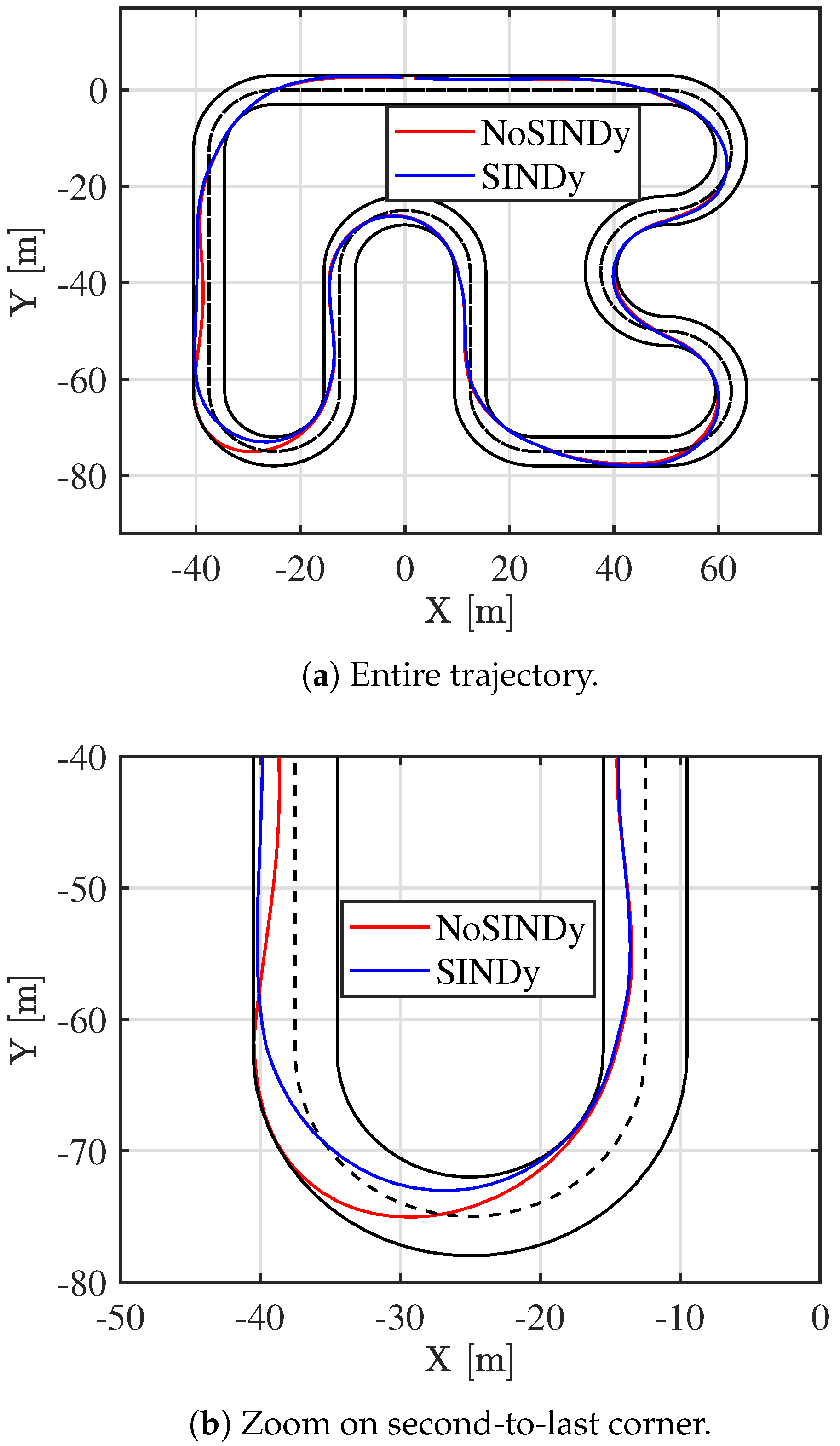
The results of this adaptation process are illustrated in
Figure 9. A clear distinction can be observed between the trajectories taken during the second and third laps. Prior to SINDy’s activation, the vehicle struggles to maintain optimal control, nearly reaching the track boundaries at the penultimate turn. However, after SINDy is executed, a significant improvement in trajectory control is achieved. The vehicle follows a more stable path, effectively navigating the track with greater precision. Additionally, this improved control also leads to enhanced performance, as evidenced by a reduction in lap time. The vehicle completes the lap 1 s faster than before, demonstrating that the updated predictive model enhances both safety and performance. Over a 24 s lap, this corresponds to an improvement of approximately
.
At this stage, the testing scenario is further refined to introduce greater complexity. Instead of using a simplified vehicle model, the CarMaker software is employed to simulate a high-fidelity representation of the system. The chosen vehicle is a Tesla Model S, ensuring that the analysis is conducted with a realistic and detailed model. Additionally, the tracks on which the vehicle operates are fully modeled within the CarMaker environment, providing a more comprehensive and representative testing platform. When working with a high-fidelity simulation scenario, additional effects can emerge and significantly influence vehicle dynamics. Among these, the longitudinal dynamics are particularly impacted by the presence of resistive forces, such as rolling resistance and aerodynamic drag, that normally are modeled as additional inputs. As discussed in
Section 3, these contributions are incorporated into the system identification process by augmenting the SINDy library with two additional functions related to the longitudinal acceleration state,
. Specifically, the function
is assumed to be proportional to rolling resistance, while the function
is associated with aerodynamic drag. This modification aims to enhance the accuracy of the identified dynamic equations for
.
Two testing scenarios assess the framework’s performance in this complex environment. The first validates the offline identification of a high-fidelity vehicle model, evaluating its ability to reconstruct dynamics with greater detail than the previous 3-DOF bicycle model. The second scenario tests online adaptation using Constrained-SINDy, enabling real-time refinement while enforcing physically meaningful constraints. This ensures accurate and robust identification, preventing non-physical terms and maintaining reliability in dynamic conditions.
4.3. CarMaker: Offline Testing
To execute the offline approach, the simulation is performed on the track shown in
Figure 1a, implemented in the CarMaker environment. The vehicle is initially controlled by the IPG Driver module to follow a predefined trajectory. Relevant state variables and their derivatives are collected to ensure a comprehensive dataset for analysis. Additionally, the state vector is augmented with the front and rear lateral slip angles, which are assumed to be known and computed using Equation (
10).
The results obtained from the application of SINDy are presented in
Figure 10 and
Figure 11. The sparse regression algorithm successfully identifies a model with a maximum error of 6% in
, 10% in
, and 38% in
. The error in the identification of angular acceleration can be attributed to the fact that the corresponding expression depends almost exclusively on the forces on the wheels, which makes it highly nonlinear. However, the
value serves as a more reliable indicator of accuracy, as the identification of angular acceleration is mainly influenced by wheel forces. Despite the nonlinear nature of this dependency, the approximation remains sufficiently accurate, allowing for good overall performance.
The reconstruction of the model parameters is achieved through the expressions for lateral and longitudinal accelerations. These error values demonstrate the effectiveness of the approach in capturing the essential vehicle dynamics while maintaining a reduced model complexity. As shown in
Figure 10, the state variables
,
, and
are effectively identified and reproduced by SINDy. This validation confirms that the learned model accurately captures the key characteristics of the vehicle’s dynamic behavior.
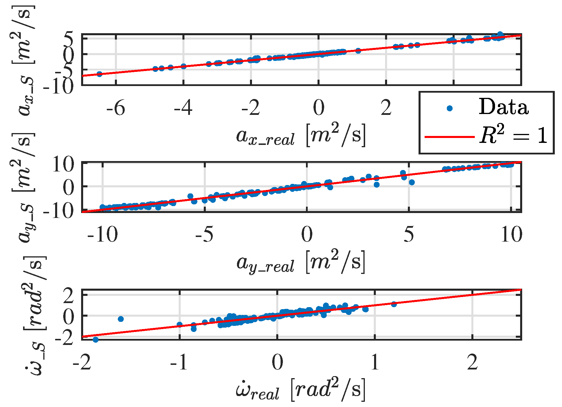
As accomplished before, an error analysis is conducted to assess the reliability and accuracy of the SINDy-based identification process. The results are presented in
Figure 11, which displays the
graph constructed using the test dataset.
Table 4 summarizes the percentage error of the SINDy identification along with the corresponding
values for all relevant states.
Additionally, beyond simply reconstructing the vehicle’s equations of motion, the extracted weights provide valuable insights into the physical parameters of the system. For instance, the mass of the vehicle can be directly inferred from the weight associated with the input torque
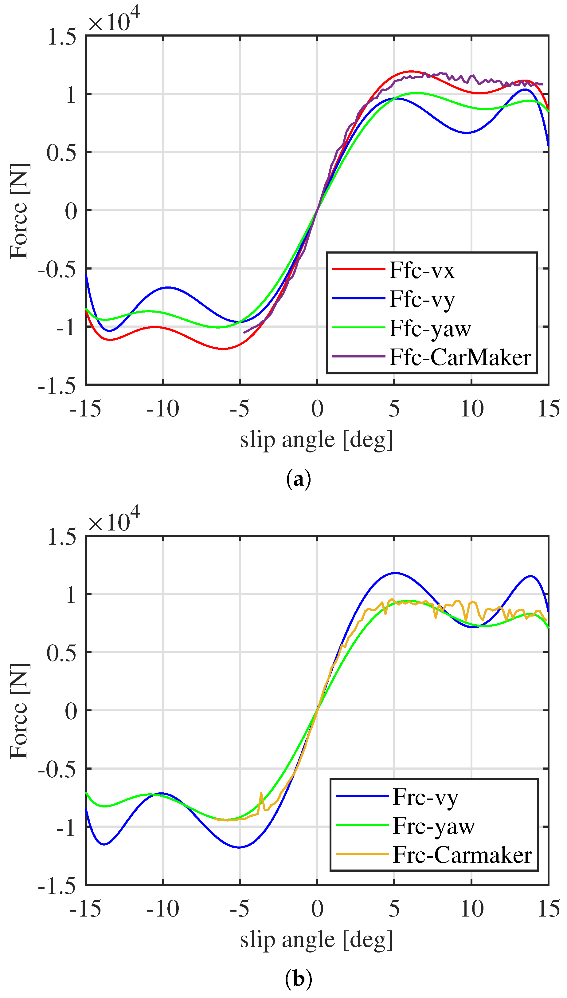
T. The percentage error on the discovered mass is 1.7%. Moreover, the shape of the tire forces can also be reconstructed with the discovered weights, as shown in
Figure 12. The approximation of the curves is less accurate, likely due to the higher complexity of the simulated vehicle. The identified model must approximate highly complex dynamics, with unmodeled effects contributing to the mismatch. Additionally, the discrepancy may arise from the highly nonlinear tire forces encountered during the simulation. In this case, the lateral tire force reaches its peak at approximately
of slip angle, requiring the SINDy equation to account for a wider nonlinear range.
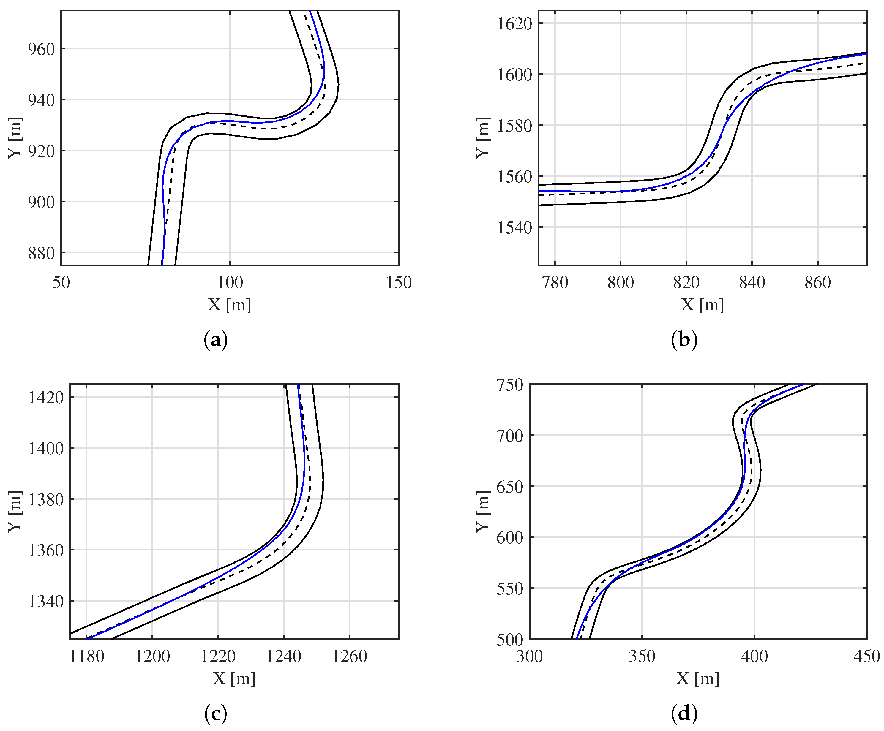
To further assess the generalization capability of the identified model, a simulation is performed on a different test track (
Figure 1b). As depicted in
Figure 13, the NMPC controller, utilizing the identified model, successfully navigates a full lap on this complex track.
4.4. CarMaker: Online Testing
The final scenario tested involves the online identification capability of SINDy. The objective is to assess SINDy’s ability to adaptively identify the vehicle model in real time and improve its predictive accuracy under changing conditions. To create a challenging identification scenario, the predictive model previously identified on the complex track is intentionally altered. Specifically, its weights are modified by approximately 20%. This change significantly impacts vehicle control performance, to the extent that the reference velocity must be drastically reduced to maintain stability. As a result, the simulated complex vehicle mostly operates in the linear tire force region, which significantly limits the ability to capture and identify nonlinear behaviors.
To enhance robustness in the identified model parameters, Constrained-SINDy is implemented. In this approach, constraints are applied to limit the variation of the discovered weights, ensuring that the model does not deviate excessively from values of the coefficients that have physical meaning. Given that the offline-identified model demonstrated good performance and low identification error, particularly in the states and , it is chosen as the reference model for formulating constraints on the weight adjustments. The constraint strategy allows for a maximum variation of ±20% on the weights, with the exception of those related to friction forces, for which the upper bound is set to zero. This restriction ensures that the model does not identify overly incorrect terms that could compromise the testing process.
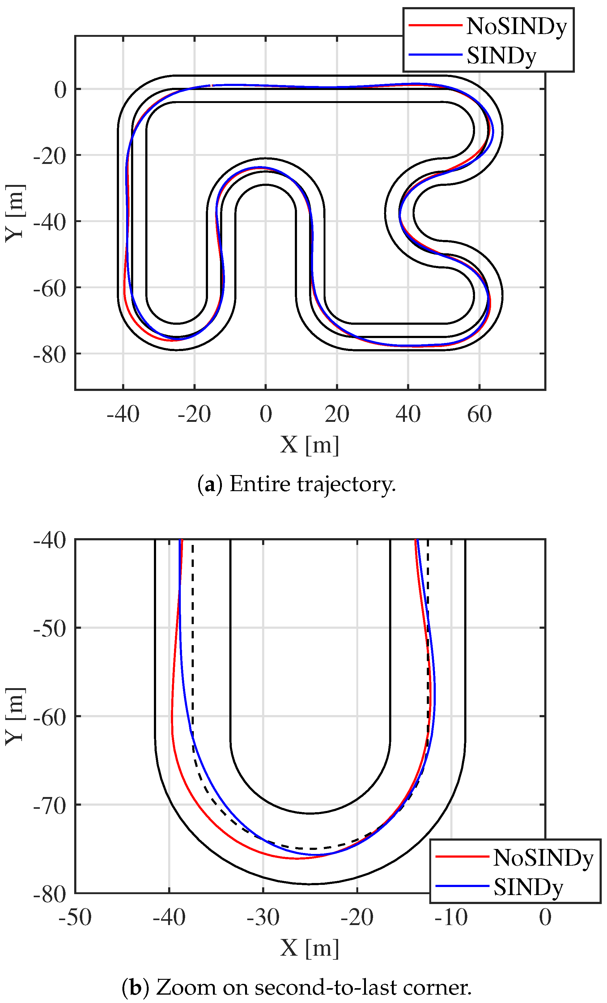
The simulation is executed using Constrained-SINDy to update the vehicle model. The vehicle is initially subjected to two laps with a fixed predictive model, meaning that no adaptive learning takes place during these first laps. Before the start of the third lap, Constrained-SINDy is activated, allowing the algorithm to adjust the predictive model in real time. The newly computed weights capture the altered dynamics, refining the approximation of the single-track bicycle model as it responds to the evolving conditions. The results clearly indicate an improvement in the controller’s tracking performance, as shown in
Figure 14. The first two laps are performed to have the same initial conditions on the second and third lap.
Before SINDy is applied, the vehicle exhibits unstable behavior, particularly during cornering. At curve exits, the vehicle approaches the track boundaries, resulting in an unsafe and inefficient trajectory. However, once Constrained-SINDy updates the predictive model, the vehicle maintains a more controlled and precise path through the turns, demonstrating improved stability and responsiveness. When the reference speed is kept constant, the vehicle follows a smoother trajectory; specifically, the lap time is reduced from 43.85 s to 42.05 s, corresponding to an overall improvement of
. However, the vehicle is able to navigate the track at a higher reference velocity, particularly increasing from
to
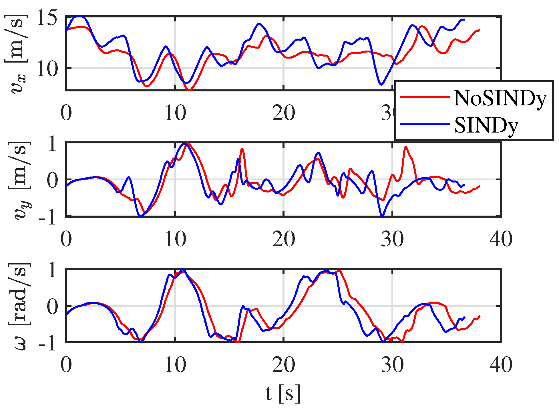
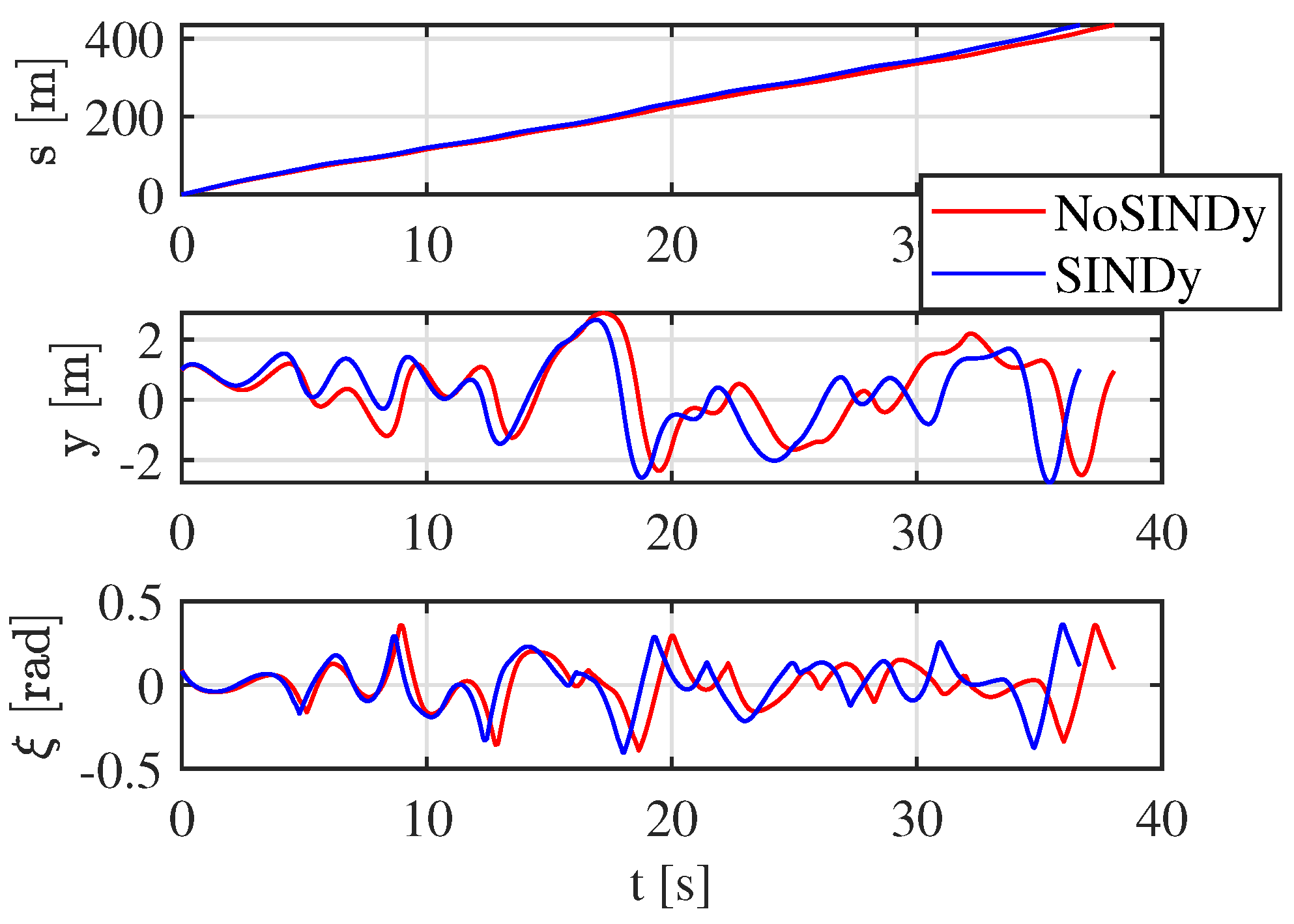
with the updated model. The difference between the two laps can also be seen in
Figure 15 and
Figure 16, where the vehicle states are depicted. This result highlights the benefits of real-time model adaptation, showing that by refining the predictive model during operation, the vehicle can achieve both better stability and enhanced performance.
5. Conclusions and Future Developments
This work investigated the integration of the SINDy algorithm into an MPC framework for autonomous vehicle systems. Unlike traditional MPC approaches that rely on fixed, physics-based models, SINDy offers a data-driven alternative capable of identifying governing equations directly from data, while maintaining interpretability and physical structure.
Based on a review of related work, the proposed method offers advantages in terms of computational efficiency and scalability for real-time applications when compared to stochastic MPC approaches, which are often limited in this regard. In addition, while deep learning methods typically yield black-box models with limited interpretability, the SINDy-based framework preserves transparency and tunability—desirable properties in safety-critical applications such as automated driving. This study also introduced a constrained version of SINDy to promote physically meaningful parameter updates in the presence of unmodeled dynamics.
In the first scenario, SINDy is applied to identify a 3-degree-of-freedom (3-DOF) vehicle model from simulation data. The offline phase consists of collecting data and constructing the state vector, the corresponding derivative vector, and the library matrix. Sparse regression is then used to identify the governing equations, effectively approximating the Pacejka tire force formulation. The identified model is subsequently tested within the MPC framework on a different and more challenging track. In the online phase, the predictive model is continuously updated within MPC, allowing real-time refinement. The results show improved trajectory tracking performance and reduced lap times.
In the second scenario, a high-fidelity vehicle model is simulated in CarMaker. SINDy is used to approximate its dynamics using a simplified 3-DOF representation. As in the first case, the offline phase involves applying SINDy to generate a reduced-order model from simulation data, which is then tested on a separate challenging track. During the online phase, a constrained version of SINDy is employed to regulate parameter updates, maintaining consistency and preventing unphysical variations. The results confirm an improvement in the quality of control inputs and a further reduction in lap times.
Throughout the study, it became evident that selectively updating the model based on informational advantage could further enhance efficiency by avoiding unnecessary or noisy updates. Future work will focus on developing intelligent data substitution mechanisms and robust noise-handling strategies, such as Weak-SINDy or advanced filtering techniques. Additionally, introducing structured uncertainty bounds within the identification process is expected to improve the robustness of the Constrained-SINDy approach, enabling the derivation of valid parameter intervals and laying the groundwork for a set-membership-based framework.
Overall, the proposed methodology enhances the adaptability and performance of learning-based MPC systems, offering a promising direction for real-time control in autonomous vehicle applications.


 ,
, 


