Development of Water Quality Analysis for Anomaly Detection and Correlation with Case Studies in Water Supply Systems

Abstract

The increasing importance of water quality management in water supply systems requires the development of efficient methodologies for the early detection of water quality incidents related to the detection of anomalies in water quality parameters. Research aims to analyze real-time water quality data (pH, turbidity, electrical conductivity, temperature, and chlorine), perform anomaly detection across parameters, and conduct a comprehensive investigation of water quality incidents that correlate with detected anomalies in water supply systems. This study can contribute to the development of an early detection and response system related to water quality incidents in water supply systems. Future work will focus on enhancing the application of systems for early detection of water quality incidents by expanding the data, developing anomaly detection methods by applying machine learning techniques, and figuring out the correlations between anomalies and water quality incidents.

1. Introduction

Water quality management in water supply systems is essential for public health and safety. Drinking water distribution systems (DWDS) have been recognized as one of the primary sources responsible for water-related infectious diseases [1]. Failures in DWDS have been associated with outbreaks, particularly involving enteric pathogens transmitted through water.

The increasing incidents stemming from various issues within water supply systems increase public concern over tap water quality. The accident in Incheon, Korea, and the leachate leakage from livestock disposal sites have significantly increased public concern about tap water. Notably, there were severe contamination issues with lead in water supply systems in Michigan, Unites States, presenting significant health risks [2]. Heavy metal contamination in water supplies has raised significant apprehension regarding public health in China [3]. These incidents related to water quality issues in the water supply system emphasize the need for early warning and response system to deal with water quality incidents effectively. In response to growing concerns regarding water quality in supply systems, advanced monitoring practices have been developed to address the issues.

Globally, there is an increasing trend towards the application of artificial intelligence for managing and predicting water quality issues in water supply systems. Establishing AI-based predictive management in water supply systems requires the development of a real-time water quality monitoring system and extensive monitoring data for the development of AI modeling. Recent studies on anomaly detection in water supply systems have extensively explored various methodologies, including pressure-based monitoring, machine learning applications, and systematic evaluations of detection techniques [4]. Research has highlighted the effectiveness of automated pressure-based methods for identifying anomalous consumption events in water distribution networks [5,6], demonstrating sensitivity to anomaly magnitude and time of occurrence [7]. Furthermore, machine learning algorithms, particularly unsupervised models, have been widely applied to detect anomalies in distinguishing abnormal patterns from normal fluctuations [8]. Emerging advancements in machine learning research have focused on designing algorithms that leverage empirical data [4]. However, the application of machine learning in evaluations has proven complex due to the challenges of handling real-world data involving large datasets, noise, and asymmetry. To detect anomalies in these datasets, the removal of outlier data during model construction has been necessary, which has improved model accuracy by employing unsupervised machine learning techniques [9]. Unsupervised machine learning has been used to group data with similar characteristics into clusters, enabling the detection of anomalies within datasets and providing system recommendations. This approach has relied on the inherent structure of datasets rather than labeled data to identify patterns and organize groups. The systematic review of anomaly detection approaches has identified key challenges including data quality issues, real-time monitoring limitations, and the need for enhanced model interpretability.

Traditional methods for predicting water quality issues primarily rely on statistical models due to the limitations that often result in inadequate accuracy [6]. Despite advancements in real-time water quality monitoring, research on predicting incidents through anomaly detection correlations remains limited.

This study aims to analyze time-series data for water quality parameters, conduct anomalies detection of water quality, and research water quality incidents through the analysis of correlation between water quality parameters in water supply systems. To achieve these objectives, this research collected real-time monitoring of key water quality parameters.

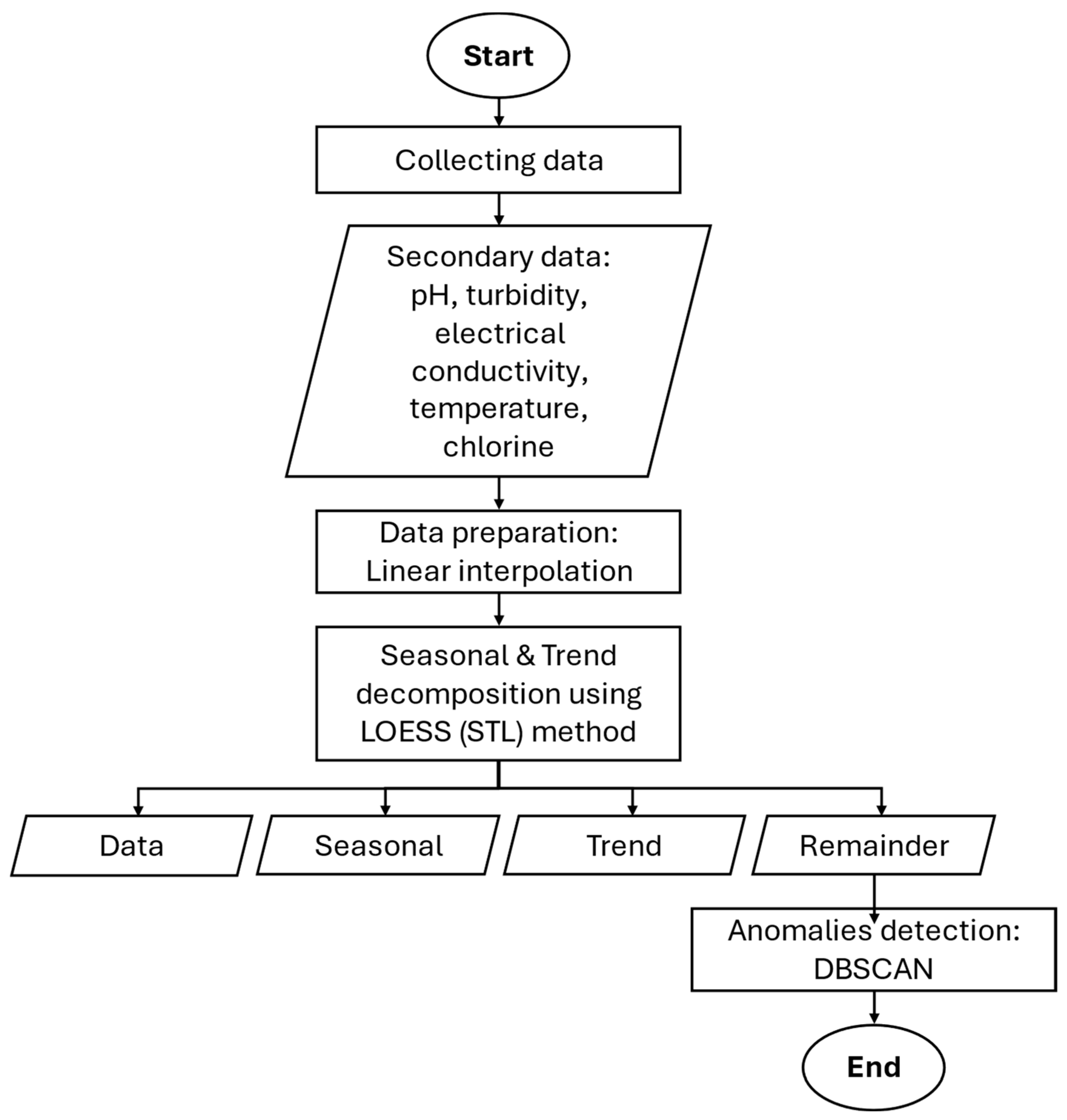
2. Materials and Methods

2.1. Site Description and Data Collection

Secondary data refers to information that has already been gathered or produced. These datasets are often collected by government agencies or organizations before being repurposed for new studies. Unlike primary data collection, which requires direct interaction with subjects or environments, secondary data are readily available. These sources provide valuable insights, allowing them to be further analyzed [10]. Secondary data were collected from water quality observations conducted within a water supply system in Daegu, South Korea. Water quality was monitored at seven stations during March 2024 over a seven-day period, with data recorded at one-minute intervals continuously for 24 h each day. These seven stations comprised three monitoring points situated at the endpoints (marked in red) and four points along the pipeline inflow (marked in black), as depicted in Figure 1.

2.2. Water Quality Parameters

Major water quality parameters, as suggested by the Environmental Protection Agency (EPA) for water quality monitoring in water supply systems, including chlorine, pH, electrical conductivity, temperature, and turbidity (

Table 1. The relationship between key water quality parameters and incidents related to anomalies detection in water supply system.

Water Quality Parameters	Descriptions
Residual chlorine	A decrease in chlorine level means the regrowth of biological organisms within water distribution systems.
pH	The pH level can change when acidic or alkaline agents enter the water supply system, with the extent of this change being inversely proportional to the water’s buffering capacity.
Electrical conductivity	Electrical conductivity is generally used as an indicator for dissolved solids. Some chemical pollutants entering the water distribution system can elevate electrical conductivity.
Temperature	Temperature can influence the rate of chemical reaction, making it an important factor for substances entering the water distribution system. The variation in temperature may indicate the external fluids entering the water distribution system.
Turbidity	Sudden increases in turbidity may indicate the entry of pollutants into the water supply systems.

), were monitored and collected at one-minute intervals. Table 1 illustrates the relationship between major water quality parameters and incidents related to anomalies detection.

2.3. Application of STL Decomposition for Water Quality Analysis

The analysis was performed by conducting preprocessing steps, which consists of handling missing data through linear interpolation and visualizing the processed data using R-4.4.2 for Windows. The Seasonal and Trend decomposition using Loess (STL) method was then applied to decompose the time series data into seasonal, trend, and remainder components [11]. This method was selected due to its robustness and effectiveness in analyzing and evaluating water quality, as it reveals temporal trend changes [12,13]. LOESS, a non-linear and non-parametric statistical approach, was utilized to capture local trends through local weighted loess filtering [11]. The time series data were decomposed into three components, low-frequency data representing the trend, high-frequency data representing the seasonal component, and irregular variations captured in the remainder component (Figure 2).

2.4. Anomalies Detection in Water Supply Systems

Anomaly detection is essential for identifying abnormal patterns within a dataset, providing significant insight into the system’s behavior. Anomalous points or values are not only extreme values, but also the data points that occur infrequently [7]. The DBSCAN (Density-Based Spatial Clustering of Applications with Noise) algorithm, a density-based clustering method, has been widely used for good efficiency on large databases, i.e., on databases of significantly more than just a few thousand objects [14]. A density-based clustering approach enables the identification of anomalies within time-series data by distinguishing regions with differing data densities [8]. DBSCAN was utilized in water supply systems for detecting anomalies in real time monitoring data [15]. Dense clusters of normal data were identified, while outliers were isolated as anomalies. These anomalies were often caused by internal or external disturbances within water supply systems and were used as early indicators of potential water quality incidents.

To identify anomalies, the process began by defining the dataset’s context and specifying key parameters, such as Eps (the radius for identifying neighborhood points) and minPts (the minimum number of points required to form a cluster) [14]. Based on the use of the DBSCAN algorithm applied to the evaluation of drinking water distribution systems, it is known that the Eps and minPts values are 0.04 and 15, respectively, assuming they were appropriate for detecting meaningful anomalies in the dataset [15]. Points were iteratively evaluated to determine whether they met the density criteria for cluster inclusion or were classified as noise (anomalies). Points that satisfied the criteria were included in clusters, which were expanded by incorporating neighboring points. Points partially meeting the criteria were labeled as boundary points, while those outside the clustering thresholds were flagged as anomalies. Through this approach, significant deviations in water quality parameters were effectively detected, along with the specific times at which they occurred, ensuring precise monitoring and timely identification of potential risk.

The analysis was conducted for each water quality parameter at every monitoring station. The remainder component derived from the STL decomposition served as the input data for anomaly detection using machine learning methods. As the remainder contains random fluctuations not accounted for by trend and seasonal components, it was considered an ideal dataset for identifying significant anomalies.

3. Results

3.1. Temporal Variation in Water Quality Across Monitoring Stations

A time-series analysis was conducted to examine the variation in water quality parameters at seven monitoring points within the water distribution system. Figure 3 presents a time series of water quality parameters at one-minute intervals over a period of approximately ten thousand minutes.

Water quality monitoring conducted across seven stations showed relatively constant pH levels between 7.5 and 7.8, with a median value of 7.7 across all stations (Figure 3a). Turbidity levels were generally low, around 0.1 NTU, except at End Point (470) and Inflow Point (480), where maximum values of 0.38 NTU and 0.36 NTU were recorded, respectively (Figure 3b). Electrical conductivity ranged between 160 and 200 μS/cm across most stations, with notable outliers observed at Inflow Points (461, 470, 480, and 480) (Figure 3c). Temperature exhibited an increasing trend throughout the distribution system, with higher values at endpoint stations compared to inflow points (Figure 3d). Residual chlorine concentrations remained stable between 0.4 and 0.6 mg/L across most stations, with some fluctuations observed at End Point (461) (Figure 3e).

3.2. Decomposition of Water Quality Trends Using STL Analysis

Following the analysis of water quality across all monitoring stations in the supply system, further analysis was performed using the Seasonal and Trend decomposition using Loess (STL) method. This approach facilitated the examination of individual water quality parameters to uncover trends within the monitoring period. STL was employed due to its effectiveness in decomposing time-series data into meaningful components, specifically data, seasonal, trend, and remainder. Figure 4 presents the result of STL for main water quality parameters for Inflow Point (461). The result of STL for main water quality parameters from other monitoring stations were summarized in Supplementary Materials.

In Figure 4a, moderate to high fluctuations in pH were observed, likely resulting from variations in water quality or chemical dosing adjustments at the treatment plant. Consistent daily patterns in the seasonal component indicated regular influences from chlorine and buffer dosing. The trend revealed an initial rise in pH before stabilization. Turbidity data in Figure 4b showed fluctuations and spikes, with seasonal patterns reflecting system activity and peak usage. The trend displayed a decline at approximately 3000 min followed by a rise. Remainder spikes indicated potential suspended solid intrusion or turbulent water flow. In Figure 4c, electrical conductivity exhibited significant fluctuations associated with change in dissolved salts and inorganic compounds. Seasonal variations corresponded with operational shifts and peak water usage. Trend increases at the beginning and end of the period were observed. Figure 4d showed temperature increases consistent with seasonal change, with daily cycles and environmental conditions influencing the seasonal component. The trend component displayed rising temperatures over time. Residual chlorine, as depicted in Figure 4e, fluctuated due to disinfection adjustments and usage variations. The seasonal component demonstrated consistent daily changes from routine chlorine use, while sudden drops in the remainder were identified.

3.3. Anomaly Detection in Water Quality Parameters

Anomalies in water quality parameters were identified across the seven monitoring stations, each revealing unique irregularities that highlight potential risks to the water supply system. Figure 5 shows the anomalies detection using DBSCAN; anomalies detection using DBSCAN for other stations are presented in Supplementary Materials.

For pH, deviations were observed at End Point (490), where a sudden drop suggested acid contamination (Figure 5a). Similarly, turbidity anomalies at Inflow Point (480) revealed sudden spikes (Figure 5b). Electrical conductivity anomalies (Figure 5c) were more widespread, appearing across all monitoring stations. At End Point (461), temperature anomalies were attributed to external heat sources or operational factors, which can accelerate microbial growth and chemical reactions, posing additional challenges to water quality management (Figure 5d). Chlorine anomalies at End Point (461) were marked by abrupt spikes, suggesting sudden adjustments in disinfection processes to address destabilizing the system (Figure 5e).

4. Discussion

The observed moderate to high fluctuations in pH values (Figure 4a) might be due to the variations in water quality or chemical dosing adjustments from the treatment plant. The trend revealed an initial rise in pH before stabilization, potentially caused by alkaline chemical dosing or reduced acidity [16].

For turbidity (Figure 4b), the trend displayed a decline of 3000 min followed by a rise that may be resulting from filter issues or leaks due to nearby construction. Remainder spikes indicated potential suspended solid intrusion or turbulence water flow [17,18].

The fluctuations in electrical conductivity (Figure 4c) appear to be related to changes in dissolved salts and inorganic compounds. Trend increases at the beginning and end of the period suggested the introduction of new water sources or pipe corrosion. Remainder spikes indicated contamination by salts or chemicals [19].

The temperature increases consistently with seasonal change with daily and environmental conditions (Figure 4d), promoting microbial growth, reducing dissolved oxygen, and accelerating chemical reactions. The fluctuations in residual chlorine (Figure 4e) may be a result of disinfection adjustments and variations in usage. Sudden drops in the remainder could be estimated as mixing issues or operational disruptions. The consistent daily changes observed in the seasonal component could be explained by routine chlorine dosing practices.

Anomalies detection in water supply systems is crucial in water quality management as it can identify early potential incidents related to water issues. It is possible to detect contamination, infrastructure failures, or other hazardous conditions from deviations in key water quality parameters by applying anomaly detection. Anomaly detection allows for the prevention of water quality issues from escalating from minor to major incidents, thereby protecting public health and maintaining the integrity of the water distribution system. The following is an overview of anomalies detection of each water quality parameter related to case studies.

Significant changes in pH have been observed to alter water chemistry. A sudden decrease in pH within DWDS has been linked to acid contamination, while sharp increases are linked to alkali intrusion. The pH level is also closely associated with the release of metal if the system’s pipes contain metallic components. At lower pH levels, metals embedded in pipe scale sediments are more to be released compared to higher pH values [16].

Turbidity in DWDS has been attributed to the accumulation of particulate matter and subsequent resuspension, which can cause discoloration and compromise water quality [20]. Elevated turbidity levels have indicated increased sediment concentrations, typically caused by turbulent flow. Turbidity has also been influenced by the number and size of particles, particularly those exceeding five microns in diameter

Electrical conductivity has been affected by dissolved salts, ions, and inorganic materials [19]. Increases in conductivity during pipe scale release suggest the introduction of ions into the water. These ions increase electrical conductivity, which in turn accelerates electrochemical reactions and the corrosion of pipe scales [21]. E. coli contamination has been identified through turbidity and conductivity measurements, as conductivity is highly responsive to various contaminants. Conductivity measurements have also been shown to depend on temperature, further pointing out the importance of continuous monitoring as an interrelated parameter [22].

Temperature within DWDS has been linked to water quality degradation, with rising temperatures increasing the risk of waterborne diseases [23]. Temperatures exceeding 20 °C have been found to accelerate the oxidative potential of chlorine dioxide, which in turn hastens the aging process of plastic-made pipes [24].

Sudden drops or spikes in residual chlorine concentrations within DWDS have indicated contamination, equipment failure, or shift in water demand. Chlorine monoxide concentrations have been observed to directly impact the aging mechanisms of polyethylene (PE) distribution pipes. Polymer pipes have been found to release biodegradable organic materials, thereby altering nutrient availability for bacterial growth.

Addressing issues related to water quality parameters, including pH, conductivity, temperature, and turbidity, requires the enhancement of real-time monitoring systems with anomaly detection and correlation studies for incidents in water supply systems.

The study relies on real-time water quality data from seven monitoring stations in Daegu, South Korea. While this dataset provides valuable insights, a broader spatial and temporal dataset could enhance the generalizability of the findings.

5. Conclusions

This study examined the time-series data of water quality parameters from monitoring systems in water supply networks, performed anomaly detection, and its correlation with water quality incidents. The study aimed to identify potential incidents related to water quality issues in water supply systems by setting upper and lower limits for these parameters to investigate anomalies detection from real-time water quality monitoring data. The research focused on analyzing anomalies detection for real-time monitoring data of main water quality parameters including pH, turbidity, electrical conductivity, temperature, and chlorine. For further research on anomalies detection, DBSCAN were applied on the remainder component of STL decomposition, and anomalies were identified in pH, turbidity, electrical conductivity, temperature, and chlorine. The case study for anomaly detection can result from various causes, such as environmental factors, operational issues, and pipeline corrosion. Anomalies detection from pH may result from corrosion in the pipeline, or scale formation. Anomalies detection in electrical conductivity indicate ion release resulting from corrosion or infiltration of external water sources. Turbidity anomalies often indicate sediment resuspension or leaking from pipelines. The case studies emphasized the crucial need for anomaly detection systems from real-time water quality monitoring in water supply systems. These systems ensure early detection of incidents related to water quality issues in water supply systems, maintaining the integrity of water supply systems. Unlike traditional statistical models that rely on fixed thresholds, our approach allows for the identification of anomalies based on data-driven density-based clustering, making it more adaptable to different water supply system conditions. Future research will aim to expand datasets, improve anomaly detection accuracy, and further explore the relationship between anomalies and specific water quality incidents to enhance water supply management.

References

1. World Health Organization. Surveillance and Outbreak Management of Water-Related Infectious Diseases Associated with Water-Supply Systems; World Health Organization: Belgrade, Serbia, 2019. [Google Scholar]
2. Hanna-Attisha, M.; LaChance, J.; Sadler, R.C.; Champney Schnepp, A. Elevated Blood Lead Levels in Children Associated With the Flint Drinking Water Crisis: A Spatial Analysis of Risk and Public Health Response. Am. J. Public Health 2016, 106, 283–290. [Google Scholar] [CrossRef] [PubMed]
3. Huang, Z.; Liu, C.; Zhao, X.; Dong, J.; Zheng, B. Risk assessment of heavy metals in the surface sediment at the drinking water source of the Xiangjiang River in South China. Environ. Sci. Eur. 2020, 32, 23. [Google Scholar] [CrossRef]
4. Jalal, D.; Ezzedine, T. Decision Tree and Support Vector Machine for Anomaly Detection in Water Distribution Networks. In Proceedings of the 2020 International Wireless Communications and Mobile Computing (IWCMC), Limassol, Cyprus, 15–19 June 2020; IEEE: New York, NY, USA, 2020; pp. 1320–1323. [Google Scholar] [CrossRef]
5. Mabunda, N.; Ramotsoela, D.T.; Abu-Mahfouz, A.M. Intrusion Detection in Water Distribution Systems Using Machine Learning Techniques. In Proceedings of the 2022 International Conference on Artificial Intelligence of Things (ICAIoT), Istanbul, Turkey, 29–30 December 2022; IEEE: New York, NY, USA, 2022; pp. 1–6. [Google Scholar] [CrossRef]
6. Mazzoni, F.; Marsili, V.; Alvisi, S.; Franchini, M. Detection and pre-localization of anomalous consumption events in water distribution networks through automated, pressure-based methodology. Water Resour. Ind. 2024, 31, 100255. [Google Scholar] [CrossRef]
7. Celik, M.; Dadaser-Celik, F.; Dokuz, A.S. Anomaly detection in temperature data using DBSCAN algorithm. In Proceedings of the 2011 International Symposium on Innovations in Intelligent Systems and Applications, Istanbul, Turkey, 15–18 June 2011; IEEE: New York, NY, USA, 2011; pp. 91–95. [Google Scholar] [CrossRef]
8. Jain, P.; Shankar Bajpai, M.; Pamula, R. A Modified DBSCAN Algorithm for Anomaly Detection in Time-series Data with Seasonality. Int. Arab. J. Inf. Technol. 2022, 19, 23–28. [Google Scholar] [CrossRef] [PubMed]
9. Chinnakkaruppan, K.; Krishnamoorthy, K.; Agniraj, S. A Hybrid Approach for Forecasting the Technical Anomalies in Sensor-based Water Quality Distribution Data. In Proceedings of the 2023 International Conference on Power, Instrumentation, Energy and Control (PIECON), Aligarh, India, 10–12 February 2023; IEEE: New York, NY, USA, 2023; pp. 1–5. [Google Scholar] [CrossRef]
10. Ajayi, V. A Review on Primary Sources of Data and Secondary Sources of Data. Eur. J. Educ. Pedagog. 2023, 2, 1–6. [Google Scholar]
11. Cleveland, R.B.; Cleveland, W.S.; Mcrae, J.E.; Terpenning, I. STL: A Seasonal-Trend Decomposition Procedure Based on LOESS. J. Off. Stat. 1990, 6, 3–73. [Google Scholar]
12. Deng, C.; Liu, L.; Li, H.; Peng, D.; Wu, Y.; Xia, H.; Zhang, Z.; Zhu, Q. A data-driven framework for spatiotemporal characteristics, complexity dynamics, and environmental risk evaluation of river water quality. Sci. Total Environ. 2021, 785, 147134. [Google Scholar] [CrossRef] [PubMed]
13. Wang, L.; Dong, H.; Cao, Y.; Hou, D.; Zhang, G. Real-time water quality detection based on fluctuation feature analysis with the LSTM model. J. Hydroinform. 2023, 25, 140–149. [Google Scholar] [CrossRef]
14. Ester, M.; Kriegel, H.-P.; Sander, J.; Xu, X. A density-based algorithm for discovering clusters in large spatial databases with noise. In Proceedings of the Second International Conference on Knowledge Discovery and Data Mining, Portland, OR, USA, 2–4 August 1996; KDD’96. AAAI Press: Washington, DC, USA, 1996; pp. 226–231. [Google Scholar]
15. Ghamkhar, H.; Jalili Ghazizadeh, M.; Mohajeri, S.H.; Moslehi, I.; Yousefi-Khoshqalb, E. An unsupervised method to exploit low-resolution water meter data for detecting end-users with abnormal consumption: Employing the DBSCAN and time series complexity. Sustain. Cities Soc. 2023, 94, 104516. [Google Scholar] [CrossRef]
16. Zhang, S.; Tian, Y.; Guo, Y.; Shan, J.; Liu, R. Manganese release from corrosion products of cast iron pipes in drinking water distribution systems: Effect of water temperature, pH, alkalinity, SO42− concentration and disinfectants. Chemosphere 2021, 262, 127904. [Google Scholar] [CrossRef] [PubMed]
17. Juncosa, R.; Cereijo, J.L.; Vázquez, R. Physicochemical Parameters in the Generation of Turbidity Episodes in a Water Supply Distribution System. Water 2022, 14, 3383. [Google Scholar] [CrossRef]
18. Xin, C.; Khu, S.-T.; Wang, T.; Zuo, X.; Zhang, Y. Effect of flow fluctuation on water pollution in drinking water distribution systems. Environ. Res. 2024, 246, 118142. [Google Scholar] [CrossRef] [PubMed]
19. Asenbaum, A.; Pruner, C.; Kabelka, H.; Philipp, A.; Wilhelm, E.; Spendlingwimmer, R.; Gebauer, A.; Buchner, R. Influence of various commercial water treatment processes on the electric conductivity of several drinking waters. J. Mol. Liq. 2011, 160, 144–149. [Google Scholar] [CrossRef]
20. Blokker, E.J.M.; Schaap, P.G. Particle Accumulation Rate of Drinking Water Distribution Systems Determined by Incoming Turbidity. Procedia Eng. 2015, 119, 290–298. [Google Scholar] [CrossRef]
21. Palma, L.; Hatam, F.; Di Nardo, A.; Prévost, M. Contaminations in water distribution systems: A critical review of detection and response methods. AQUA Water Infrastruct. Ecosyst. Soc. 2024, 73, 1285–1302. [Google Scholar] [CrossRef]
22. Tian, Y.; Wei, L.; Yu, T.; Shen, H.; Zhao, W.; Chu, X. Adsorption of Cr(VI) and Cr(III) on layered pipe scales and the effects of disinfectants in drinking water distribution systems. J. Hazard. Mater. 2024, 474, 134745. [Google Scholar] [CrossRef]
23. Furst, K.E.; Graham, K.E.; Weisman, R.J.; Adusei, K.B. It’s getting hot in here: Effects of heat on temperature, disinfection, and opportunistic pathogens in drinking water distribution systems. Water Res. 2024, 260, 121913. [Google Scholar] [CrossRef]
24. Lancioni, N.; Parlapiano, M.; Sgroi, M.; Giorgi, L.; Fusi, V.; Darvini, G.; Soldini, L.; Szeląg, B.; Eusebi, A.L.; Fatone, F. Polyethylene pipes exposed to chlorine dioxide in drinking water supply system: A critical review of degradation mechanisms and accelerated aging methods. Water Res. 2023, 238, 120030. [Google Scholar] [CrossRef] [PubMed]
Figure 1. Location of water quality monitoring systems in Daegu, South Korea, with seven monitoring stations: three at pipeline endpoints (red markers) and four at inflow points (black markers).
Electronics 14 01933 g001
Figure 2. Workflow for water quality anomaly detection. The process begins with data collection. The data undergoes preparation using linear interpolation, seasonal, and trend decomposition using the LOESS (STL) method. The decomposed components (data, seasonal, trend, and remainder) are analyzed to detect anomalies using the DBSCAN clustering algorithm.
Electronics 14 01933 g002
Figure 3. Water quality across monitoring stations: (a) pH; (b) Turbidity; (c) Electrical conductivity; (d) Temperature; and (e) Chlorine.
Electronics 14 01933 g003
Figure 4. STL decomposition for Inflow Point (461): (a) pH; (b) Turbidity; (c) Electrical conductivity; (d) Temperature; and (e) Chlorine.
Electronics 14 01933 g004
Figure 5. Anomalies detection using DBSCAN: (a) pH in End Point (490); (b) Turbidity in Inflow Point (480); (c) Electrical conductivity in Inflow Point (461); (d) Temperature in End Point (461); and (e) Chlorine in End Point (461).
Electronics 14 01933 g005