Abstract
A prescribed performance neuro-adaptive control scheme is proposed for a single-link flexible-joint robotic manipulator with unknown deadzone and actuator faults. A new smooth deadzone inverse model is constructed to offset the adverse effect caused by the input deadzone in the actuator of flexible-joint manipulators. The control law is developed by coordinating prescribed performance control with a backstepping technique to ensure transient/steady-state performance, while adaptive neural networks are employed for uncertainty approximation. The tracking error is always restricted within the prescribed bound during the control process, and it ultimately converges to the small neighborhood of origin. All signals in the closed-loop flexible-joint robotic manipulator system are proved to be uniformly bounded. Simulation results are provided to demonstrate the efficiency of the prescribed performance adaptive neural network backstepping control scheme.
1. Introduction
Flexible-joint robotic manipulators have been widely used in the field of human–computer interaction for safety considerations [1,2]. Compared with traditional rigid manipulators, flexible-joint robotic manipulators have smoother force transmission and greater impact tolerance. With elastic factor considered, the dynamics of a flexible manipulator may be regarded as the combination of the motor side and link side. It is difficult to obtain the accurate values of the parameters in the above two sides, such as the mass matrix of the motor, the damping matrix of the motor, and the inertia matrix and heavy moment matrix of the link. In addition, flexible-joint robotic manipulators suffer from external disturbances and viscous friction during operation [3]. All these factors make the accurate tracking control of flexible-joint robotic manipulators nontrivial.
In recent decades, significant technological advancements have been made in the field of flexible-joint robotic control [4]. As the most widely adopted traditional control technique in various application domains, PID control [5,6,7] retains its relevance in the field of flexible-joint robotic manipulators [8,9,10,11]. Scholars have also proposed advanced methods, such as adaptive backstepping control [12,13], adaptive fuzzy finite control [14], active disturbance rejection control [15,16], and sliding mode control [17,18,19], to address specific challenges. These works have promoted the advancement of the tracking control method for flexible-joint robotic manipulators. As a non-differentiable function characterizing certain non-sensitivity for small control inputs, the deadzone input nonlinearity is ubiquitous in numerous mechanical and electrical components, such as valves and DC servo motors. The presence of deadzone nonlinearity in feedback control systems may severely degrade system performance. The investigation on deadzone compensation has gained much attention in the adaptive control community, which has led to the emergence of some useful strategies, including the robust strategy [20], approximation of neural network/fuzzy system [21], and inverse model-based direct adaptive approach [22]. In the context of flexible-joint manipulator systems, some efforts have made to offset the aforementioned adverse effect. In [23], an adaptive neural network command filtered tracking control method is developed for a flexible-joint robotic manipulator with input deadzone, with the robust strategy used to deal with deadzone nonlinearity. In [24], a robust tracking control approach was proposed for a flexible-joint robotic manipulator with unmodeled dynamics and deadzone, where an adaptive fuzzy system was constructed to compensate for the input deadzone. In [25], both deadzone and flexibility were considered in the position tracking control design of the space manipulator, where the deadzone was compensated by using the robust approach. If the slopes of the deadzone on both the left and right sides are the same, it is convenient to apply the robust strategy to handle deadzone nonlinearities. Otherwise, it is not convenient to adopt the robust strategy for deadzone compensation [22]. In contrast, the inverse model-based direct adaptive approach can be conveniently used to handle the input deadzone whose left slope and right slope are not equal. To the best of our knowledge, few results in the literature concern inverse compensation control for flexible-joint robotic manipulators with deadzone nonlinearity, which presents the motivation for our research, as adaptive approaches are still limited.
Since it is impossible to completely avoid faults in flexible-joint manipulator systems, ways to maintain the expected system performance, even if potential faults occur, are a very realistic research topic. For this purpose, the fault-tolerant adaptive tracking control strategy has been studied in recent years [26]. In [27], an observer-based sliding mode control approach is proposed to solve the fault-tolerant tracking problem for a class of single-link flexible-joint manipulator systems with uncertainty, actuator fault, sensor fault, and unmatched disturbance. In [28], the fault-tolerant control of a flexible-joint robotic manipulator using the singular perturbation method was investigated to compensate for the lost performance due actuator faults and uncertainty. It should be noted that deadzone input nonlinearity is not considered in the above research results. In some practical situations, flexible-joint manipulator systems suffer from the the mixed impact of unknown deadzone and actuator faults. Usually, compensation methods designed for handling either unknown input deadzones or actuator faults cannot be directly applied to systems that experience both issues simultaneously [29,30,31]. Despite the significant advances achieved in adaptive fault control for flexible manipulator systems, at present, there are limited published research results concerning the tracking control design for flexible-joint manipulator systems suffering from such a mixed impact.
The improvement of transient- and steady-state performance in control system design has garnered much attention for some time [32,33]. In [34], Bechlioulis et al. investigated the prescribed performance control (PPC) design for SISO strict feedback nonlinear systems with known and unknown signs of the virtual control coefficients, respectively. Subsequently, this control strategy was applied to the controller design for other types of nonlinear systems. To date, in the context of flexible-joint robotic manipulators, several research results on PPC have been reported in the literature [35,36,37]. Specifically, in [35], Kostarigka et al. developed a full state feedback control scheme for flexible-joint robots with unknown dynamics and variable elasticity, so as to achieve preset performance attributes on the link position error. In [36], Ma et al. proposed an adaptive fuzzy control strategy for a single-link flexible-joint robotic manipulator with prescribed performance, in which the unknown nonlinearity is identified by adopting a fuzzy-logic system. In [37], Zhang et al. proposed a robust command-filtered control method with prescribed performance for flexible-joint robots, wherein matched and mismatched disturbances are estimated by generalized proportional integral observers. In these results, the prescribed performance function is typically constructed using an exponential function that decays over time. In these schemes, the value of the prescribed performance function is greater than the preset constant throughout the entire time domain. Therefore, it is meaningful to improve the prescribed performance control design of flexible manipulator systems by constructing new prescribed performance functions. Motivated by the above discussion, this work investigates the position tracking problem of flexible-joint robotic manipulators. A prescribed performance neuro-adaptive backstepping control (PPNABC) scheme will be developed for a single-link flexible-joint robotic manipulator subject to the mixed impact of input deadzone and actuator faults. The main contributions of this work are listed as follows:
- (i)
- Few previous works have considered the mixed impact of unknown input deadzone and actuator faults during the controller design for flexible-joint robotic manipulators. In this work, such a mixed impact will be taken into account during the prescribed performance adaptive backstepping neural network controller design for flexible-joint robotic manipulators.
- (ii)
- In the design process of the performance controller, a new construction scheme of the prescribed performance function is proposed, which has clearer specified attenuation performance than the existing design schemes. In our scheme, the value of the prescribed performance function remains constant after the preset time point. By contrast, in many existing results, unless the time reaches infinity, the value of the prescribed performance function cannot reach the preset value. Hence, our proposed prescribed performance function can provide clearer prescribed attenuation performance than existing ones.
- (iii)
- In this work, the left deadzone slope and the right one are allowed to be unequal, relaxing the strict assumption that the deadzone slopes on both sides [23,24,25].
A new smooth continuous indicator function is constructed to implement the direct adaptive control based on the smooth deadzone inverse for flexible-joint robotic manipulator systems.
The layout of this paper is as follows. The problem formulation is addressed in Section 2. The detailed control design procedure and rigorous convergence analysis are described in Section 3. A simulation study is carried out in Section 4 to validate the effectiveness of the proposed scheme. The summary of this work is given in Section 5.
2. Problem Formulation
Consider a single-link flexible-joint robotic manipulator, as shown in Figure 1.
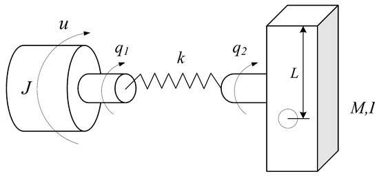
Figure 1.
Model of a flexible-joint robotic manipulator.
The dynamic model of single-link flexible-joint robotic manipulator consists of robot dynamics and actuator dynamics, which can be described by the following Lagrangian formulation:
where and stand for the angular position of the link and motor shaft, respectively; and L are the mass of the link, gravity acceleration, and the length of the link, respectively; I represents the inertias of link; K and J denote the coefficients of the joint stiffness and joint flexibility, respectively; and and represent the external disturbances. By taking the mixed impact of unknown deadzone nonlinearity and actuator faults into account, the actuator expression is described as [30]
where is the multiplicative actuator fault, denotes the additive actuator fault, and is the output of deadzone nonlinearity expressed as
in which ; and are unknown constants; v is the input; and the output, as shown in Figure 2.
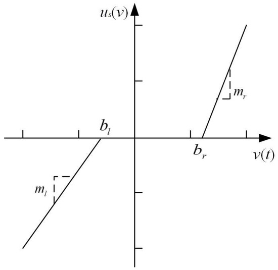
Figure 2.
Deadzone nonlinearity model.
Let , and . Then, (1) can be transformed into the following state space equation:
The control objective is to design a proper control input v such that y can precisely track the desired trajectory . To meet the requirements for the controller design in this work, a lemma and an assumption are provided as follows:
Lemma 1
([38]). For any and for any , the following inequality holds:
Assumption 1.
is assumed to be four-fold continuously differentiable with respect to time. Equation (4) is a fourth-order system. In preparing for the next phase of the backstepping control design, it is necessary that the reference signal is four times continuously differentiable. It is a common requirement in backstepping control for such systems.
Assumption 2.
The external disturbances and admit the following decomposition:
where and are continuous functions of the system states and time t; are bounded disturbance terms (possibly discontinuous) satisfying
with known constants . For notational simplicity, we hereafter omit the arguments in and and in and .
3. Main Results
This section is divided into three subsections. In Section 3.1, a smooth deadzone inverse model is presented as a preparation for the subsequent controller design. Then, the detailed controller design procedure is introduced in Section 3.2. After that, rigorous convergence analysis is given in Section 3.3.
3.1. Smooth Inverse Model for Actuator Deadzone
By parameterizing (8), we have
in which . Since , , , and are either unknown or unmeasurable, (11) cannot be directly used for the actual control input.
In this paper, a new smooth continuous indicator function is presented as follows: For ,
where is a design parameter, and
By using the above indicator functions, an estimated form of (11) is designed as
whose corresponding deadzone inverse is
Remark 1.
In existing works [22,31], is set as , in which for and . In this work, for , which adds some more convenience to the projection operation design in the following text.
Remark 2.
In [22], Zhou et al. developed an indicator function based on the hyperbolic function as follows:
where is a design parameter. In [39], Lai et al. used an arc tangent function as follows:
where is a design parameter. Our indicator in (12) adopts a two-parameter scheme (), making it simple to build and intuitive to use compared to single-parameter methods.
3.2. Backstepping Controller Design
Define the tracking error as
and the prescribed performance function as
where
Here, , , , and are the design parameters. The parameter represents a prescribed finite-time instant, typically recommended to be selected within the interval .
Remark 3.
In many existing studies, the prescribed performance function is often defined as
where . In this case, for all finite , and converges to asymptotically as . In contrast, the proposed function given by (19) ensures that for all , i.e., the performance bound reaches its steady-state value in finite time. Therefore, the formulation in (19) provides a stricter and more explicit characterization of both transient- and steady-state performance compared to (20).
Remark 4.
From (19), it can be seen that the following points hold: (i). , , and are continuous for ; (ii). holds when ; and (iii). holds when .
The parameters , and should be set appropriately. As pointed out above, should be greater than and has an appropriate margin, that is to say, the positive number should not be too small. Meanwhile, the parameter should be set neither too large nor too small. In addition, the value of determines the transition time length of the prescribed performance, and its value needs to be set reasonably.
Let us introduce a variable as follows:
where represents the inverse function of
By algebraic operation, from (21), we have
Note that is a smooth, strictly increasing function satisfying , and . From (23), we obtain
which is the theoretical basis of implementing the prescribed performance control. Meanwhile, by using the property , it can be deduced that while converges to zero, will synchronously converge to zero.
Step 1: Differentiating (24) with respect to time, we obtain
Taking the time derivative of yields
where , is a signal to be designed later.
Step 2: Define a candidate Lyapunov function as
Taking the time derivative of yields
where , , is a signal to be designed later.
By using a neural network to approximate , we have
where is the ideal parameter vector,
, are the design parameters and , with being an unknown constant.
Based on (34), the virtual control law is designed as follows:
where
with . Substituting (35) into (34), we obtain
where .
Step 3: Define a candidate Lyapunov function as
Taking the time derivative of yields
where , with being a signal to be designed. By using a neural network to approximate , we have
where is the ideal parameter vector,
, are the design parameters, and , with being an unknown constant.
Then, the virtual control law may be designed as follows:
where
with . Substituting (43) into (42), we obtain
Select a Lyapunov function as
Computing the time derivative of along (46) leads to
Let
where is the continuous component of , and is the residual. By using a neural network to approximate , we have
where is the ideal parameter vector,
, are the design parameters, and , with being an unknown constant. On the basis of (48)–(50), we have
On the basis of the above equation, we design the controller as follows:
with . To ensure the estimates and , the deadzone parameter update law is designed as follows:
where is a projection operator defined as follows: For ,
where . This projection operator satisfies the following property:
Such an operation can be found in [40]. Readers interested in projection algorithms may refer to [41] for more details.
Remark 5.
To facilitate the implementation of the proposed PPNABC, we suggest the following parameter ranges as follows: , , , , , , , , , , and , for .
3.3. Convergence Analysis
Theorem 1.
For the flexible-joint robotic manipulator system (4) subject to the mixed impact of unknown deadzone and actuator faults, under Assumptions 1 and 2, the adaptive controller is constructed as (15) and (53), with virtual control laws (28), (35), (43), (53), and weight update laws (36), (44), (54), (55). Then, the prescribed tracking performance in (25) can be achieved for the entire ime domain. Meanwhile, all the system signals in the closed-loop flexible-joint manipulator system (1) are bounded in spite of the mixed impact of unknown input deadzone and actuator faults.
Proof.
Define a Lyapunov function
where
By invoking (36), we have
According to (44), we have
Based on the update law (43), we have
Based on the above four inequalities, it can be deduced that
Then, integrating it over , we obtain
Further, it yields
Multiplying both sides of inequality (77) by yields
In this work, the adaptive inverse method is used to cope with the unknown deadzone in the controller design, which is different from the applicable strategy proposed in some existing studies [24,25].
4. Numerical Simulation
In this section, simulation results are provided to demonstrate the good performance of the proposed PPNABC scheme for a flexible-joint robotic manipulator subject to the mixed impact of unknown input deadzone and actuator faults. The actual values of system parameters for dynamic Equation (4) are , , . The actuator faults are and , and the actual parameters of the deadzone are and . It should be noted that the values of these parameters and actuator faults are not utilized in the design of the control law and adaptive laws.
The design parameters are chosen as follows: , , , , , , , and . For , .
The robotic manipulator is arranged to start from .
The reference trajectory is . The control target is that the system output can track the desired trajectory, even in the case of external disturbances and .
Figure 3, Figure 4, Figure 5, Figure 6, Figure 7, Figure 8, Figure 9 and Figure 10 show the simulation results when .
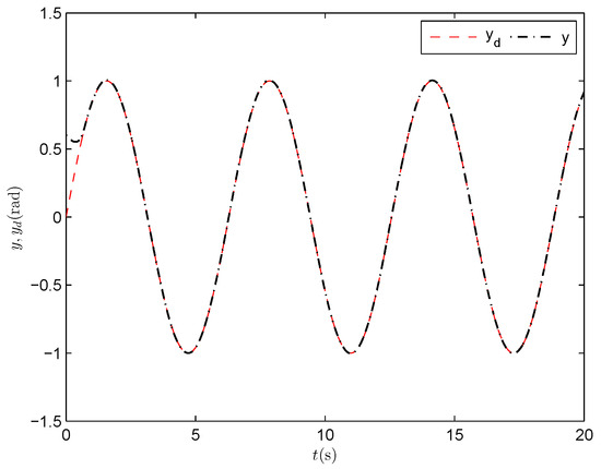
Figure 3.
Output tracking performance (PPNABC) .
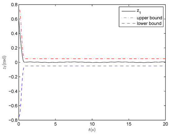
Figure 4.
Output tracking error with prescribed performance constraints (PPNABC) .
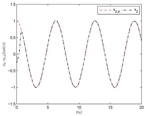
Figure 5.
Angular velocity tracking performance of the link (PPNABC) .
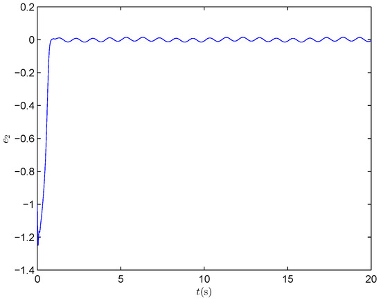
Figure 6.
Angular velocity tracking error of the link (PPNABC) .
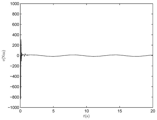
Figure 7.
Control input (PPNABC) .
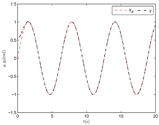
Figure 8.
Output tracking performance (PPNABC) .
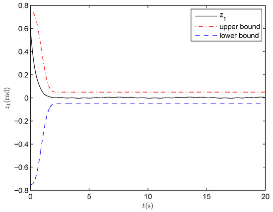
Figure 9.
Output tracking error with prescribed performance constraints (PPNABC) .
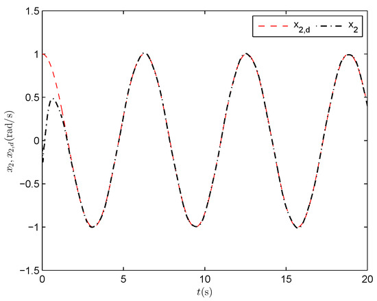
Figure 10.
Angular velocity tracking performance of the link (PPNABC) .
Figure 3 shows that y accurately tracks the desired trajectory with a rapid transient response. From Figure 4, it can be seen that the output tracking error always remains within the prescribed bound. The angular velocity tracking performance of the link is shown in Figure 5, from which we can see that can track quickly and accurately. The above-mentioned better tracking performance is further confirmed by the profile of the velocity tracking error of the link presented in Figure 6, where . The curve of the control input is depicted in Figure 7.
Comparison 1.
In order to examine the impact of varying parameter on the control performance, we provide the simulation results corresponding to in Figure 8, Figure 9 and Figure 10. By comparing Figure 3 and Figure 8, we find that the system output tracks well for both and , with showing faster transient response. By comparing Figure 4 and Figure 9, we observe that the tracking error stays within prescribed bounds for both and , but it converges faster for . By comparing Figure 5 and Figure 10, we note that the angular velocity tracks accurately in both cases, with achieving quicker and more precise tracking. Overall, the control system achieves effective tracking for both and , with providing faster convergence.
Comparison 2.
In [42], a backstepping dynamic surface control (BDSC) algorithm is proposed for flexible-joint robotic manipulators with neither unknown deadzone nor actuator faults as follows:
where , , , ,
The above backstepping dynamic surface control algorithm is adopted for simulation with the control parameters chosen as , . The output response is illustrated in Figure 11, and the output tracking error is depicted in Figure 12. Comparing Figure 3 and Figure 11, we can see that better output tracking performance is obtained in Figure 3, which indicates that the proposed PPNBC scheme is effective while the system suffers from the mixed impact of deadzone and actuator faults. On the other hand, in Figure 4, the output tracking error is always restricted within prescribed bounds during the control process, whereas this constraint attribute is not observed in Figure 11. These results verify the effectiveness of the proposed PPNABC scheme.
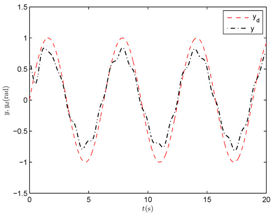
Figure 11.
Output tracking performance (BDSC).
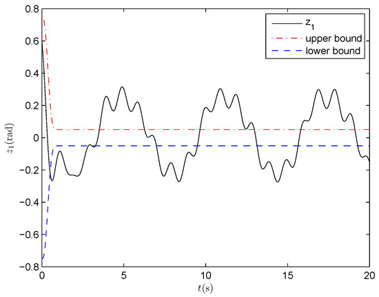
Figure 12.
Output tracking error (BDSC).
5. Conclusions
In this paper, with the prescribed performance strategy and backstepping technique cooperatively applied, a PPNABC law has been developed for the trajectory tracking of flexible-joint robotic manipulator systems subject to the mixed impact of unknown deadzone and actuator faults. The developed controller can not only guarantee that the angle trajectory of the link tracks the desired trajectory, but also the tracking error is restricted within the prescribed bound during the control process. The unknown input deadzone can be well handled by using the deadzone inverse approach. The effectiveness and superiority of the proposed control scheme have been verified through simulation results. In future works, we will consider the state constraint issue in the adaptive control design for flexible joint robotic manipulator systems subject to the mixed impact of unknown deadzone and actuator faults.
Author Contributions
Conceptualization, H.X. and Q.Y.; methodology, Q.Y.; software, J.C.; validation, Q.Y., C.Z. and C.M.; formal analysis, H.X.; investigation, J.C; resources, Q.Y.; data curation, H.X.; writing—original draft preparation, H.X.; writing—review and editing, Q.Y.; visualization, H.X.; supervision, Q.Y.; project administration, C.M.; funding acquisition, C.Z. All authors have read and agreed to the published version of the manuscript.
Funding
This work was partially supported by the Zhejiang Provincial Natural Science Foundation of China under Grant No. LY22F030011 and the Undergraduate Innovation Projects at Zhejiang University of Water Resources and Electric Power under Grant No. S202411481081.
Data Availability Statement
Data are contained within the article.
Conflicts of Interest
The authors declare no conflict of interest.
References
- Ruderman, M. Compensation of nonlinear torsion in flexible joint robots: Comparison of two approaches. IEEE Trans. Ind. Electron. 2016, 63, 5744–5751. [Google Scholar] [CrossRef]
- Rsetam, K.; Cao, Z.; Man, Z. Design of robust terminal sliding mode control for underactuated flexible joint robot. IEEE Trans. Syst. Man Cybern. Syst. 2022, 52, 4272–4285. [Google Scholar] [CrossRef]
- Sun, L.; Yin, W.; Wang, M.; Liu, J. Position Control for Flexible Joint Robot Based on Online Gravity Compensation with Vibration Suppression. IEEE Trans. Ind. Electron. 2018, 65, 4840–4848. [Google Scholar] [CrossRef]
- Chatlatanagulchai, W.; Meckl, P.H. Model-independent control of a flexible-joint robot manipulator. J. Dyn. Syst. Meas. Control 2009, 131, 442–447. [Google Scholar] [CrossRef]
- O’Dwyer, A. A summary of PI and PID controller tuning rules for processes with time delay. Part 1: PI controller tuning rules. IFAC Proc. Vol. 2000, 33, 159–164. [Google Scholar] [CrossRef]
- Åström, K.J.; Hägglund, T. PID control. IEEE Control Syst. Mag. 2006, 26, 30–31. [Google Scholar]
- Wrat, G.; Ranjan, P.; Bhola, M.; Mishra, S.K.; Das, J. Position control and performance analysis of hydraulic system using two pump-controlling strategies. Proc. Inst. Mech. Eng. Part I J. Syst. Control Eng. 2019, 233, 1093–1105. [Google Scholar] [CrossRef]
- Tomei, P. A simple PD controller for robots with elastic joints. IEEE Trans. Autom. Control 1991, 36, 1208–1213. [Google Scholar] [CrossRef]
- De Luca, A.; Siciliano, B.; Zollo, L. P97D control with on-line gravity compensation for robots with elastic joints: Theory and experiments. Automatica 2005, 41, 1809–1819. [Google Scholar] [CrossRef]
- Dehghani, A. Self-tuning PID controller design using fuzzy logic for a single-link flexible joint robot manipulator. J. Teknol. 2016, 78, 6–13. [Google Scholar] [CrossRef]
- Alam, W.; Ali, N.; Wahaj Aziz, H.M.; Iqbal, J. Control of Flexible Joint Robotic Manipulator: Design and Prototyping. In Proceedings of the 2018 International Conference on Electrical Engineering (ICEE), Lahore, Pakistan, 15–16 February 2018; pp. 1–6. [Google Scholar]
- Cheng, X.; Zhang, Y.; Liu, H.; Wollherr, D.; Buss, M. Adaptive neural backstepping control for flexible-joint robot manipulator with bounded torque inputs. Neurocomputing 2021, 458, 70–86. [Google Scholar] [CrossRef]
- Oh, J.H.; Lee, J.S. Control of flexible joint robot system by backstepping design approach. Intell. Autom. Soft Comput. 1999, 54, 267–278. [Google Scholar] [CrossRef]
- Qi, R.; Lam, H.K.; Liu, J.; Yu, J. Adaptive fuzzy finite-time singular perturbation control for flexible joint manipulators with state constraints. IEEE Trans. Syst. Man Cybern. Syst. 2024, 54, 7521–7527. [Google Scholar] [CrossRef]
- Pan, C.; Fei, X.; Xiao, J.; Huang, J.; Yang, Z. Model-assisted reduced-order ESO based command filtered tracking control of flexible-joint manipulators with matched and mismatched disturbances. Appl. Sci. 2022, 12, 8511. [Google Scholar] [CrossRef]
- Bilal, H.; Yin, B.; Aslam, M.S.; Anjum, Z.; Rohra, A.; Wang, Y. A practical study of active disturbance rejection control for rotary flexible joint robot manipulator. Soft Comput. 2023, 27, 4987–5001. [Google Scholar] [CrossRef]
- Wang, H.; Zhang, Q.; Sun, Z.; Tang, X.; Chen, I.-M. Continuous Terminal Sliding-Mode Control for FJR Subject to Matched/Mismatched Disturbances. IEEE Trans. Cybern. 2022, 52, 10479–10489. [Google Scholar] [CrossRef]
- Soltanpour, M.R.; Moattari, M. Voltage based sliding mode control of flexible joint robot manipulators in presence of uncertainties. Robot. Auton. Syst. 2019, 118, 204–219. [Google Scholar]
- Cheng, X.; Liu, H.; Lu, W. Chattering-suppressed sliding mode control for flexible-joint robot manipulators. Actuators 2021, 10, 288. [Google Scholar] [CrossRef]
- Wang, X.S.; Su, C.Y.; Hong, H. Robust adaptive control of a class of nonlinear systems with unknown dead-zone. Automatica 2004, 40, 407–413. [Google Scholar] [CrossRef]
- Lewis, F.L.; Tim, W.K.; Wang, L.Z.; Li, Z.X. Deadzone compensation in motion control systems using adaptive fuzzy logic control. IEEE Trans. Control. Syst. Technol. 1999, 7, 731–742. [Google Scholar] [CrossRef]
- Zhou, J.; Wen, C.; Zhang, Y. Adaptive output control of nonlinear systems with uncertain dead-zone nonlinearity. IEEE Trans. Autom. Control 2006, 51, 504–511. [Google Scholar] [CrossRef]
- Wang, H.; Kang, S. Adaptive Neural Command Filtered Tracking Control for Flexible Robotic Manipulator with Input Dead-Zone. IEEE Access 2019, 7, 22675–22683. [Google Scholar] [CrossRef]
- Yan, Z.; Lai, X.; Meng, Q.; Zhang, P.; Wu, M. Tracking control of single-link flexible-joint manipulator with unmodeled dynamics and dead zone. Int. J. Robust Nonlinear Control 2021, 31, 1270–1287. [Google Scholar] [CrossRef]
- Shen, J.; Zhang, W.; Zhou, S.; Ye, X. Fuzzy adaptive compensation control for space manipulator with joint flexibility and dead zone based on neural network. Int. J. Aeronaut. Space Sci. 2023, 24, 876–889. [Google Scholar] [CrossRef]
- Liu, Y.; Yao, X.; Zhao, W. Distributed neural-based fault-tolerant control of multiple flexible manipulators with input saturations. Automatica 2023, 156, 111202. [Google Scholar] [CrossRef]
- Chen, Y.; Guo, B. Sliding mode fault tolerant tracking control for a single-link flexible joint manipulator system. IEEE Access 2019, 7, 83046–83057. [Google Scholar] [CrossRef]
- Elghoul, A.; Tellili, A.; Abdelkrim, M.N. Reconfigurable control of flexible joint robot with actuator fault and uncertainty. J. Electr. Eng. 2019, 70, 876–889. [Google Scholar] [CrossRef]
- Ren, Y.; Zhu, P.C.; Zhao, Z.J.; Yang, J.; Zou, T. Adaptive fault-tolerant boundary control for a flexible string with unknown dead zone and actuator fault. IEEE Trans. Cybern. 2021, 52, 7084–7093. [Google Scholar] [CrossRef]
- Zhao, Z.J.; Tan, Z.F.; Liu, Z.J.; Efe, M.O.; Ahn, C.K. Adaptive inverse compensation fault-tolerant control for a flexible manipulator with unknown dead-zone and actuator faults. IEEE Trans. Ind. Electron. 2023, 70, 12698–12707. [Google Scholar] [CrossRef]
- Yu, Y.; Wang, L. Adaptive fault-tolerant finite-time flight-path angle control for aircraft systems with unknown deadzone and actuator faults. IEEE Access 2024, 12, 94205–94215. [Google Scholar] [CrossRef]
- Yan, L.; Hsu, L.; Xiuxia, S. A variable structure MRAC with expected transient and steady-state performance. Automatica 2006, 42, 805–813. [Google Scholar] [CrossRef]
- Xie, S.; Chen, Q.; He, X. Predefined-Time Approximation-Free Attitude Constraint Control of Rigid Spacecraft. IEEE Trans. Aerosp. Electron. Syst. 2023, 59, 347–358. [Google Scholar] [CrossRef]
- Bechlioulis, C.P.; Rovithakis, G.A. Adaptive control with guaranteed transient and steady state tracking error bounds for strict feedback systems. Automatica 2009, 45, 532–538. [Google Scholar] [CrossRef]
- Kostarigka, A.K.; Doulgeri, Z.; Rovithakis, G.A. Prescribed performance tracking for flexible joint robots with unknown dynamics and variable elasticity. Automatica 2013, 49, 1137–1147. [Google Scholar] [CrossRef]
- Ma, H.; Zhou, Q.; Li, H.; Lu, R. Adaptive Prescribed Performance Control of A Flexible-Joint Robotic Manipulator With Dynamic Uncertainties. IEEE Trans. Cybern. 2022, 52, 12905–12915. [Google Scholar] [CrossRef]
- Zhang, Y.; Lei, Y.; Zhang, T.; Song, R.; Li, Y.; Du, F. Robust command-filtered control with prescribed performance for flexible-joint robots. IEEE Trans. Instrum. Meas. 2023, 72, 1–13. [Google Scholar] [CrossRef]
- Ge, S.S.; Hong, F.; Lee, T.H. Robust adaptive control of nonlinear systems with unknown time delays. Automatica 2005, 41, 1181–1190. [Google Scholar] [CrossRef]
- Lai, G.; Liu, Z.; Zhang, Y.; Chen, C.L.P.; Xie, S.; Liu, Y. Fuzzy Adaptive Inverse Compensation Method to Tracking Control of Uncertain Nonlinear Systems With Generalized Actuator Dead Zone. IEEE Trans. Fuzzy Syst. 2017, 25, 191–204. [Google Scholar] [CrossRef]
- Fang, Y.M.; Xu, Y.Z.; Li, J.X. Adaptive dynamic surface control for electro-hydraulic servo position system with input saturation. Control Theory Appl. 2014, 31, 511–518. [Google Scholar]
- Krstic, M.; Kanellakopoulos, I.; Kokotovic, P.V. Nonlinear and Adaptive Control Design; John Wiley & Sons: New York, NY, USA, 1995. [Google Scholar]
- Liu, J.K. Robot Control System Design and MATLAB Simulation: The Advanced Design Method; Tsinghua University Press: Beijing, China, 2023. [Google Scholar]
Disclaimer/Publisher’s Note: The statements, opinions and data contained in all publications are solely those of the individual author(s) and contributor(s) and not of MDPI and/or the editor(s). MDPI and/or the editor(s) disclaim responsibility for any injury to people or property resulting from any ideas, methods, instructions or products referred to in the content. |
© 2025 by the authors. Licensee MDPI, Basel, Switzerland. This article is an open access article distributed under the terms and conditions of the Creative Commons Attribution (CC BY) license (https://creativecommons.org/licenses/by/4.0/).