Customer Churn Prediction Based on Coordinate Attention Mechanism with CNN-BiLSTM

Abstract

Due to increased competition in the marketplace, companies in all industries are facing the problem of customer attrition. In order to expand their market share and increase profits, companies have shifted from the concept of ‘acquiring new customers’ to ‘retaining old customers’. In this study, we design a deep learning model based on multi-network feature extraction and an attention mechanism, convolutional neural network–bidirectional long and short-term memory network–fully connected layer–coordinate attention (CNN-BiLSTM-FC-CoAttention), and apply it to customer churn risk assessment. In the data preprocessing stage, the imbalanced dataset was processed using the SMOTE-ENN hybrid sampling method. In the feature extraction stage, a sequence-based CNN and time-based BiLSTM are combined to extract the local and time series features of the customer data. In the feature transformation stage, high-level features are extracted using a fully connected layer of 64 Relu neurons and the sequence features are reshaped into matrix features. In the attention enhancement stage, the extracted feature information is refined using a coordinate attention learning module to fully learn the channel and spatial location information of the feature map. To evaluate the performance of the proposed model, we include public datasets from telecom, bank and insurance industries for ten-fold cross-validation experiments, and the results show that the CNN-BiLSTM-FC-CoAttention model outperforms the comparison models in all metrics. Our proposed model improves the accuracy and generalisation of the model prediction by combining multiple algorithms, enabling it to be widely used in multiple industries. As a result, the model gives enterprises a better and more general decision-making reference for the timely identification of potential churn customers.

1. Introduction

In the context of business diversification, market saturation and economic globalisation, competition among firms has become more intense [1]. Many firms are facing the problem of customer churn due to newer ways of acquiring information and the excessive homogenisation of their products and services [2]. Customer churn refers to the behaviour of customers who choose not to subscribe to a firm’s products or services or who switch to competitors [3]. A churned customer base is highly likely to influence the business choices of other customers in their social networks, which can potentially lead to damage to the business’s reputation and a sharp drop in revenue as more customers choose to unsubscribe [4].

Customer Relationship Management (CRM) has become one of the indispensable strategies for the long-term development of enterprises in a dynamic and intense market. Through CRM, enterprises can establish and maintain stable relationships with their customers and increase their market share and profits by improving customer satisfaction [5]. With the continuous development of data science and the continuous improvement of data acquisition methods, enterprises can obtain a large amount of data about their customers through various channels, including the region in which the customer is located, the time of transactions, the frequency of consumption and so on. Through an in-depth analysis of the acquired data on the signs of customer behaviour, enterprises can formulate strategies that are more in line with the needs of customers [6]. One study [7] found that a company with five million customers could expect to make hundreds of thousands of dollars in profits by setting up a churn prediction system to conduct marketing retention campaigns for 10% of potentially lost customers. Shirazi et al. [8] combined structured archival data with unstructured data, such as telephone call logs, to build a customer churn risk assessment system using the Datameer big data analytics tool on the Hadoop platform with the SAS business intelligence system (version number: SAS 9.4) and showed that the system was effective in identifying churned customers of a Canadian bank during the period of 2011–2015. In a study of the European financial industry, Caigny et al. [9] integrated textual data into a churn prediction system and showed that textual data were effective in increasing the additional profitability of customer retention campaigns and assisting business managers in making more informed decisions. In a study on customer churn prediction in the web browser market, Wu et al. [10] proposed a customer churn early warning system based on a multivariate time series transformer model (MBST), based on the shortcoming that tree-based models cannot fully use the temporal characteristics of browser users, and experimented on a real Tencent QQ browser dataset containing more than 600,000 samples, and the results confirmed the feasibility of their system.

According to one study, the cost of retaining loyal customers is one-fifth to one-tenth of the cost of acquiring new ones [11]. Another study shows that for every 5% drop in customer churn, businesses can expect a 25 to 85% increase in profits [12]. It is therefore a crucial strategy for businesses to anticipate potential lost customers and act quickly to maintain their loyalty. This approach not only curtails potential financial losses, but also significantly increases the profit potential of the organisation.

Customer churn prediction is considered as a binary classification problem [13]. Specifically, companies use various models trained on historical customer data collected to estimate the future probability of churn for each customer and classify customers as churn or non-churn. In recent years, customer churn prediction has become an important strategy for large enterprises in developed countries to gain a foothold in the market and stabilise their growth. Whether an organisation can accurately identify and retain customers who are about to be lost is highly dependent on the churn prediction model used [14]. Therefore, building a reliable churn risk assessment mechanism is important for enterprises to prevent churn in advance and take targeted measures to reduce the churn rate, so as to ensure the long-term stable development of enterprises [15]. In this context, we propose a customer churn risk early warning model based on a convolutional neural network–bidirectional long and short-term memory network–fully connected layer–coordinate attention (CNN-BiLSTM-FC-CoAttention).

The main contributions of this paper are as follows:

(1)

We propose a novel early warning model for customer churn risk based on multiple networks extracting features in parallel with an attention-driven approach. In the proposed model, one-dimensional convolutional neural networks (1DCNNs), bidirectional long and short-term memory networks (BiLSTMs) and coordinate attention are combined to effectively improve the prediction.

(2)

We use the SMOTE-ENN algorithm to resample the original dataset due to the significant difference between the churn and non-churn samples in the dataset, effectively improving the impact of class imbalance on model predictions.

(3)

In response to the existing single-feature extraction method, which leads to the inability to accurately extract the complex behavioural information of customers, we propose to use a 1DCNN and BiLSTM to extract customer features in parallel in order to obtain information about customers’ local consumption patterns and long-term behavioural trends.

(4)

We conduct a ten-fold cross-test on publicly available customer churn datasets in multiple industries, and the results confirm that our proposed model can be effectively applied to a wide range of industries, suggesting that our model has the potential for a wide range of applications in different industries.

The remainder of the paper is organised as follows: Section 2 reviews the literature related to customer churn prediction. Section 3 describes the methodology proposed in this paper. Section 4 analyses the experimental results. Section 5 concludes this research.

2. Literature Review

Customer churn prediction is one of the most important research topics in business management and a difficult part of Customer Relationship Management [16]. Prior research has revealed three types of churn: the first is active churn, in which such customers actively withdraw from the relationship with the original firm and switch to competitors; the second is passive churn, in which such users stop subscribing to the firm’s business only if the firm actively terminates the contract with them; and the third is potential churn, in which such users will, without the firm’s knowledge of any reason at all, terminate the business relationship with the original enterprise [17]. Due to the complexity, noisiness and hidden nature of customer history information, manual methods of prediction are ineffective and costly, so building a customer churn prediction model becomes a wiser, more desirable and better choice. In terms of the research direction, the direction of customer churn prediction can be divided into two directions.

On the one hand, researchers have improved the performance of predictions by constructing more complex models. In the field of customer churn prediction, traditional approaches mainly rely on machine learning models to identify and assess the risk of customer churn. Rao et al. [18] embedded the focal loss function into the CatBoost model from the algorithmic level to obtain the Focal Loss–CatBoost model (FLCatBoost) and proposed an improved resampling algorithm, IADASYN, from the data-level perspective, which removes the outliers from the samples by introducing a local outlier factor algorithm (LOF) prior to resampling the samples with ADASYN to eliminate the outliers, thus eliminating the noisy data synthesised by resampling due to the deviation of outliers from normal points. They validated the model on a publicly available credit card customer churn dataset; the results demonstrate the feasibility of the proposed model in the field of credit card customer churn prediction. Lalwani et al. [19] used the Gravitational Search Algorithm (GSA) for feature selection and evaluated it using a five-fold cross-validation. They used models such as logistic regression (LR), Naive Bayes (NB), random forest (RF), decision tree (DT), AdaBoost and CatBoost and found that the AdaBoost model performed the best in terms of accuracy, with 81.71%. Jamjoom’s study [20] evaluated the application of hybrid models in the health insurance industry and found experimentally that when the ratio of the number of churned to non-churned customers in the training set was 5:5, the results were better by combining K-means with logistic regression, and when the ratio was 7:3, the hybrid model combining K-means with neural networks (NNs) predicted more accurately. Pustokhina et al. [21] proposed a telecommunication customer churn prediction model based on the combination of an improved SMOTE oversampling method and an Optimal Weighted Extreme Learning Machine (OWELM). In that study, the Multi-Objective Raindrop Optimisation Algorithm (MOROA) was used to determine the optimal sampling rate for SMOTE as well as the parameter optimisation for the OWELM. Through simulation experiments with a ten-fold cross-validation on three publicly available telecommunication datasets, the results showed that the proposed model performed well in terms of prediction performance, with accuracies of 94%, 92% and 90.9%, respectively.

These studies have applied maximum likelihood methods to the field of customer churn prediction, which have improved the accuracy of churn risk assessment to some extent. However, traditional machine learning models rely heavily on adequately processed structured data. After a long period of research and development, scholars have gradually recognised that customer churn datasets are usually characterised by a high dimensionality, non-normal distribution and nonlinearity [3]. These characteristics make the accuracy and generalisation ability of machine learning models limited. Compared to machine learning models, deep learning models show great advantages in dealing with high-dimensional and complex customer data. Deep learning models abstract data and extract features step-by-step by simulating the multilevel structure of the human brain, a mechanism that enables deep learning models to automatically extract key features from raw data. Because of this, more and more researchers are adopting deep learning models to improve predictions and model performance. Almufadi et al. [22] designed a one-dimensional convolutional neural network model containing three hidden layers stacked with 43 neurons applied to customer churn prediction in the telecommunication industry, and the results confirmed the effectiveness and feasibility of the model in the task of customer churn prediction. Abdullaev et al. [23] combined the chicken flock optimisation algorithm (CSO) with a bidirectional long short-term memory network (BiLSTM) in the prediction stage to obtain the optimal parameters of the model. Xu et al. [24] proposed the use of a back propagation neural network (BPNN)-based customer churn prediction model and applied it to customer data collected from July to October in a telecommunication company, and the results confirmed the superior performance of the model. Usman et al. [25] proposed a model that uses four convolutional layers to extract local spatial features and three fully connected layers to act as classifiers applied to two publicly available datasets from the telecoms industry, and the results show that their proposed model produces superior predictions over other traditional machine learning methods. Chinnaraj [26] proposed a customer churn prediction framework based on the combination of the Elephant Herding Optimisation Algorithm (EHO) and the Improved Recurrent Neural Network (R-RNN); in his study the EHO is used to select the important features from the original feature set and optimise the best parameters of the RNN, and the experimental results show that the performance of the proposed EHO-R-RNN outperforms that of the deep neural network and the artificial neural networks.

On the other hand, researchers want to explore what drives customers to terminate their current business. Jiang et al. [27] proposed a profit-driven weighted classification model. In their study, the artificial hummingbird algorithm was used to optimise the weighting coefficients of the profit-driven members and to quantify the contribution of each feature to the prediction task by calculating the Shapley value, which revealed the mapping relationship between the customer features and the prediction. The mapping relationship between customer characteristics and outcomes improves the interpretability of the model. Similarly, in a study on bank customer churn, Peng et al. [28] concluded from an SHAP analysis that the key factors affecting bank customer churn are the number of transactions in the most recent year and the number of bank products held by the user. Bock et al. [29] proposed Sample Rule Integration with Sparse Group Lasso Regularisation (SRE-SGL) in order to solve the problems of model complexity and conflicting terms in the traditional rule integration and spline rule integration. Using Sparse Group Lasso Regularisation, the rules, linear terms and spline terms are grouped according to the variables on which they depend and sparsified both between and within groups—not only reducing unnecessary terms in the model, but also avoiding the emergence of conflicting terms based on the same variable, thus significantly improving the interpretability of the model. Their study effectively strikes a balance between prediction accuracy and interpretability. Caigny et al. [30] proposed a hybrid prediction model combining logistic regression and categorical regression trees (CARTs), which in this study is divided into a customer segmentation phase and a churn prediction phase. In the first stage, the customer base is segmented by the decision rule of the CART, which divides customers into subgroups with similar characteristics. In the second stage, logistic regression models are constructed separately for each subgroup to accurately predict the probability of customer churn. Experimental results show that this hybrid model not only effectively improves the prediction performance, but also significantly enhances the interpretability of the model.

Table 1. Literature review of various industries.

Study	Methods of Use	Multi-Network Feature Extraction	Attention Mechanism	Data Balancing Methodology	Dataset Industry
Rao [18]	FLCatBoost	×	×	IADASYN	Bank
Lalwai [19]	GSA, LR, DT , AdaBoost, KNN, RF , NB, SVM , XGBoost , CatBoost	×	×	√	Telecom
jamjoom [20]	K-means, NN, LR	×	×	×	Health Insurance
Pustokhina [21]	OWELM, MOROA	×	×	SMOTE	Telecom
Almufadi [22]	CNN, RNN, DNN	×	×	SMOTE	Mobile Telephone
Abdullaev [23]	CSO, BiLSTM	×	×	×	Telecom
Xu [24]	BPNN	×	×	×	Telecom
Usman [25]	CNN, MLP, NB, BN, DT	×	×	Under-Sampling	Telecom
Chinnaraj [26]	EHO, R-RNN	×	×	×	Telecom
Proposed	CNN, BiLSTM, CoAttention	√	√	SMOTE-ENN	Telecom, Bank, Insurance

compares the industries covered and the methods used in the different literatures.

3. Methodology

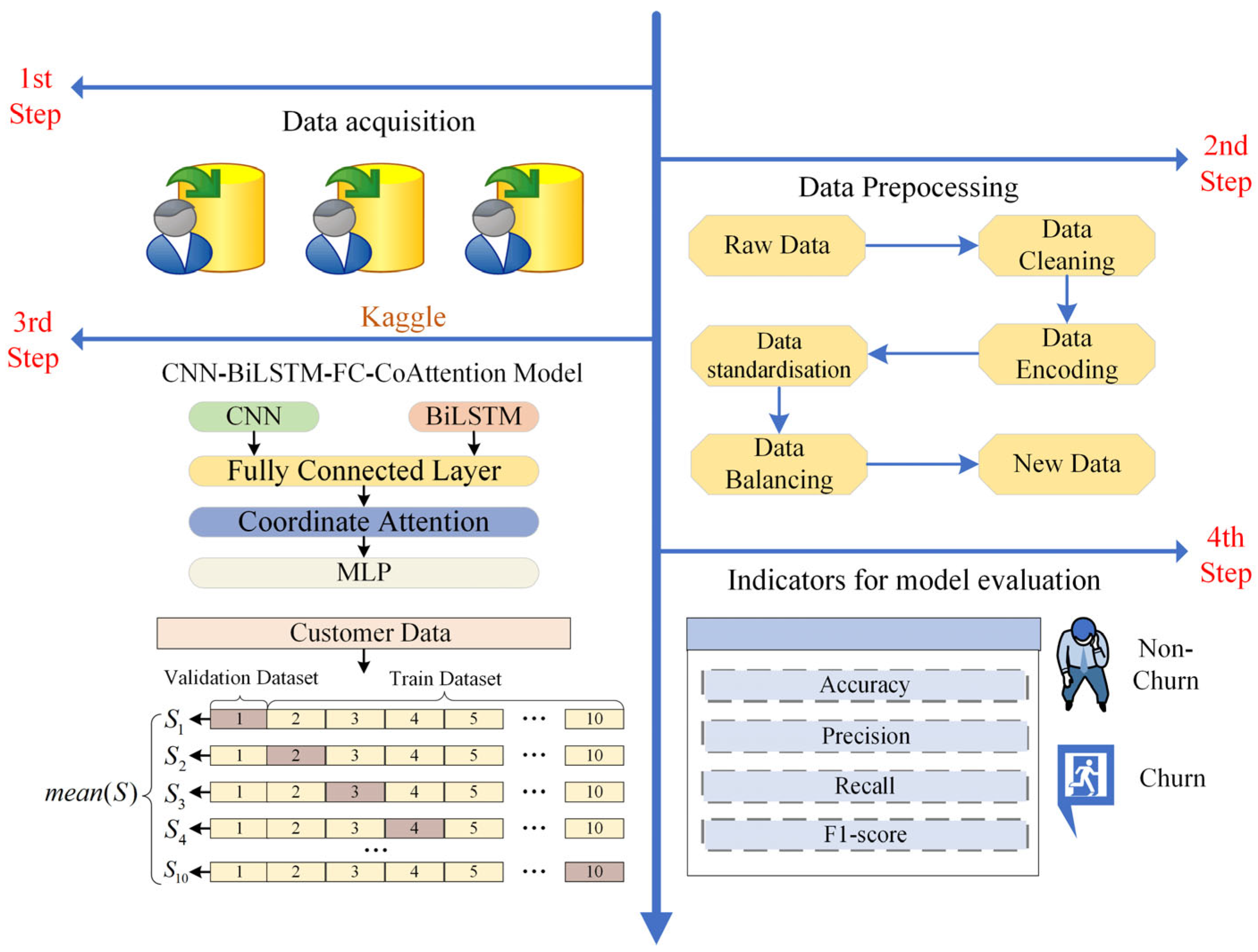
As shown in Figure 1, there are four stages in assessing the churn risk of customers in this study. First, we collected three datasets containing the telecom, bank and insurance industries. In the second step we performed necessary preprocessing on the raw data. In the third step we built a CNN-BiLSTM-FC-CoAttention model and trained it. In the fourth step we evaluated and analysed the experimental results obtained from the model training.

3.1. Dataset Information

Three publicly accessible datasets from the Kaggle data science competition platform, which spans the telecom, banking and insurance sectors, were used in this study. The datasets’ details are provided in

Table 2. Dataset information.

Dataset	Number of Samples	Churn	Non-Churn	Number of Features	Imbalance Ratio	Source
Telecom	7043	1869	5174	21	2.76	Kaggle
Bank	10,000	2037	7963	14	3.91	Kaggle
Insurance	33,908	3967	29,941	17	7.55	Kaggle

.

3.1.1. Telecom Dataset

The dataset records information about the length of customers’ subscriptions with telecommunication companies, their telephone service status and their Internet providers and contains a total of 7043 samples, each containing 21 features.

3.1.2. Bank Dataset

The dataset records information such as the region the customer belongs to, the number of products subscribed to, whether they are active or not, etc. Containing a total of 10,000 samples, the dataset contains 14 features.

3.1.3. Insurance Dataset

The dataset holds the customer history of insurance companies, totalling 33,908 samples, each possessing 17 features.

3.2. Data Preprocessing

Since the constructed customer churn early warning model cannot directly use the collected tabular data, we perform some necessary processing on the raw data. In addition, some preprocessing works before passing the data to the model for training can effectively improve the model’s fitting effect on the customer data.

3.2.1. Data Cleaning

In this stage, we process the features that have missing values. For example, in the telecom dataset there are some missing values and 0 is used to fill them up. Next, we remove irrelevant features that are only intended to distinguish between different customers, such as the ‘customerID’ feature in the telecom dataset; the ‘RowNumber’ feature in the Bank dataset; the ‘customerID’ and ‘Surname’ features in the telecom dataset; and the ‘RowNumber’ feature, ‘customerID’ and ‘Surname’ features in the Bank dataset. Finally, we unify the values that are different but have the same meaning, e.g., the ‘MultipleLines’ feature corresponds to ‘No phone service’ in the telecom dataset and ‘No Internet service’ for the feature ‘OnlineSecurity’ in the telecom dataset. For example, ‘No phone service’ for the feature ‘MultipleLines’ and ‘No Internet service’ for the feature ‘OnlineSecurity’ in the telecom dataset are united as ‘No’. By merging these similarly expressed categories into one category, the feature dimensions are reduced, thus simplifying the processing of the model.

3.2.2. Data Encoding

In this stage, we encode the categorical features to meet the data format required by the model. We convert the categorical features to numerical features by one-hot encoding. In this process, the categorical features are converted into a number of binary numerical features, and the process can be represented as shown in Figure 2.

3.2.3. Data Standardisation

In the customer churn dataset, the values of different features have different distributions, which is not conducive to model learning when used directly, as it tends to make certain features with a large range of values over-weighted in the model, thus ignoring other important feature information, resulting in the model failing to learn the true patterns in the customer data. Therefore, we mapped all numerical features to between 0 and 1 by Z-score normalisation, eliminating the scale difference in the features. The mathematical expression of this process is shown in Equation (1).

$$x^{\prime }={\displaystyle \frac{x-\mu }{\sigma }}$$

(1)

3.2.4. Data Balancing Process

In real business scenarios, far more customers choose to continue a business relationship than choose to leave. As a result, companies collect a smaller percentage of lost customers in their churn datasets. Since machine learning models and deep learning models are designed on the basis that the data are balanced, the direct use of unbalanced datasets will result in models that tend to be majority class fitted.

The datasets used in this experiment are all imbalanced datasets, i.e., the number of churned customers is much lower than the number of non-churned customers. If the original imbalanced dataset is used directly for training, even though the model accuracy is high, the model does not learn completely for a few classes of samples, resulting in lower classification accuracy for a few samples. And in the customer churn prediction task, the misclassification of churned customers is more serious than non-churned customers, so the original dataset is subjected to a sample balancing process.

SMOTE-ENN is a resampling algorithm that combines the synthetic minority over-sampling technique (SMOTE) and nearest neighbour editing (ENN) technique. In the customer churn prediction task, the use of the SMOTE on unbalanced data effectively improves the model’s ability to identify samples of churned customers. However, some noisy samples are also generated when the samples are synthesised using the SMOTE. The SMOTE-ENN resampling algorithm further combines the ENN technique to process the nearest neighbours of the samples for each majority class, thus effectively eliminating the noisy data.

In this experiment the dataset is processed using the SMOTE-ENN resampling technique to achieve the new dataset obtained after processing. Figure 3 shows the data distribution before and after balancing the data.

3.3. CNN-BiLSTM-FC-CoAttention Model

In order to predict potential churn customers more accurately and in a timely manner, we design a new deep learning model that incorporates multiple algorithms, called CNN-BiLSTM-FC-CoAttention. Figure 4 illustrates our model architecture, which consists of four phases: feature extraction, feature transformation, attention enhancement and customer classification.

(1) Feature Extraction Stage

Previous studies have revealed that customer churn datasets are highly nonlinear in nature, thus limiting the effectiveness of feature extraction by only a 1DCNN or BiLSTM. In order to eliminate the deficiency of the insufficient feature information extracted by a single network, we use sequence- and time-based networks to extract features in parallel during the feature extraction stage. Firstly, CNN-BiLSTM-FC-CoAttention receives the input data $(B\times N\times C)$ and passes them to the 1DCNN and BiLSTM, respectively. Then, the convolutional layer extracts local features from the sequential data through parameter sharing and local connectivity, and the BiLSTM can extract temporal features from the customer data by considering past behaviours and future trends. The feature extraction performance of the model is enhanced by the combination of two neural networks. To prevent overfitting, we extracted features after each layer of the 1DCNN and BiLSTM by performing a dropout layer with a dropout rate of 0.1. The output data $(B\times N\times C)$ of the 1DCNN and $(B\times N\times 2C)$ of the BiLSM are passed to the next stage. Where $B$ denotes the batch size, $N$ denotes the number of features and $C$ denotes the number of feature channels.

(2) Feature Conversion Stage

Firstly, we splice the output of the 1DCNN and the output of the BiLSM in the feature dimension in order to combine local and temporal features to generate a comprehensive feature representation $(B\times N\times 3C)$. Through this operation, we can obtain local consumption patterns and the time series information of customer behaviour. Next, we pass the extracted sequence features through a fully connected layer of 64 neurons and use the Relu activation function to learn a nonlinear transformation to extract a higher level feature representation. The dimension of the output data is $(B\times 64\times 3C)$. To prevent overfitting, it was passed through a discard layer with a 0.2 execution probability. To prepare for the next stage of feature enhancement, we reshape the output through the fully connected layer into a matrix feature. Specifically, we let $N=H\times W$, where $H$ and $W$ are the height and width of the target feature matrix, which is converted by the reshaping operation feature tensor $(B\times 64\times 3C)$ to $(B\times H\times W\times 3C)$. In this study, we set $H=W=8$. After this stage, the output data $(B\times H\times W\times 3C)$ is passed to the next stage.

(3) Attention Enhancement Stage

In order to further understand the complex behaviour of the customer history data, we further refine the extracted features in the attention enhancement stage. Specifically, we use the coordinate attention mechanism, through which we can capture the dependencies on feature channels and feature maps, effectively enhancing the feature representation of the network. The coordinate attention module encodes the transformed feature maps into direction-aware and location-sensitive attention maps, which effectively strengthens the important features related to churn and suppresses irrelevant features, thus enhancing the network’s ability to capture features related to customer churn behaviour. The output data from this stage are then passed to the next stage for churn classification.

(4) Customer Classification Stage

In order to generate the data into a final prediction, firstly the data from the previous stage are passed through a flatten layer, thus transforming the data from a high dimensional vector to a one-dimensional vector. Next, the data are passed through a fully connected layer of 64 neurons, thereby compressing and fusing the features to generate a new high-level feature representation. In addition, this layer introduces the Relu activation function to learn the complex mapping between features and churn labels. Then, 50% of the neurons are randomly discarded in order to improve the model accuracy and generalisation. Finally, the data are passed to the last fully connected layer with one neuron, which generates the final prediction probability through the Sigmoid activation function. In this study, we set the prediction probability greater than 0.5 as an imminent churn customer. The pseudo-code of our proposed CNN-BiLSTM-FC-CoAttention model can be represented by Algorithm 1.

Algorithm 1 CNN-BiLSTM-FC-CoAttention Model

1: Inputs: Dataset $D$, Churn label $L_{tarin}$, learning rate $\alpha$, Training epochs $E$, batch size $B$, fold $K$ 2: Initialise CNN-BiLSTM-FC-CoAttention model parameters 3: for k = 1 to $K$ do 4: Split $D$ into training dataset $D_{train}$ and validation dataset $D_{valit}$ 5: Split $L_{tarin}$ into training label $L_{train}$ and validation label $L_{valit}$ 6: for epoch = 1 to $E$ do 7:  for each batch ($X_{batch}$,$Y_{batch}$) in ($D_{train}$,$L_{train}$) do 8:   Forward Pass: 9:   Use 1DCNN and BiLSTM to extract feature form $X_{batch}$ 10:    Transform sequence features into matrix features through fully connected layers and reshape them into matrix features 11:    Enhance feature representation using coordinate attention 12:  Using multi-layer perceptron to predict lost labels $\stackrel{⌢}{y}$ 13:  Calculate loss value 14:  $L_{batch}=BCELoss(\stackrel{⌢}{y},y_{batch})$ 15:   Backward Pass: 16:  Compute gradients of the loss concerning model parameters 17:  Update Weights: 18:  Update model parameters using RMSprop optimizer with the learning rate $\alpha$ 19:  end for 20:  Evaluate performance on $D_{valit}$ and $L_{valit}$ 21: end for 22: end for 23.Output: Trained CNN-BiLSTM-FC-CoAttention Model

3.3.1. 1DCNN

The research on convolutional neural network can be traced back to the 1980s, while the 1DCNN is a variant on the basis of the convolutional neural network, and its classical architecture contains an input layer, a convolutional layer, an activation layer, a flatten layer, a fully connected layer and an output layer. The structure of the 1DCNN is shown in Figure 5.

• Input Layer

The input layer is located in the first layer of a 1DCNN, and its role is to receive one-dimensional sequential data as inputs to the model and pass these data to subsequent network layers. The input layer itself does not perform complex computations and serves only as an entry point for the data.

• Convolutional Layer

The convolutional layer is the core part of a 1DCNN, which extracts local features by performing a convolution operation on sequential data through a convolution kernel. In the customer churn prediction task, the input data are of a tabular type with multiple features (e.g., age, income, transaction frequency, service usage, etc.) for each customer, which can be organised into a one-dimensional sequence, and the convolutional layer extracts local features related to customer churn by sliding a convolution kernel over these sequences. In addition, the size and number of convolution kernels can determine the level of granularity with which the model performs feature extraction and the complexity of the model and is therefore an important parameter of the model. In this process, the convolution operation is shown in Equation (2).

$$y_i={\displaystyle \sum _{j=1}^K{x}_{i+j}\cdot w_j+b}$$

(2)

where $y_i$ is the output of the $i$th neuron, $x_{i+j}$ is the input consisting of the $i$th neuron to the $j$th neuron, $w_j$ is the weight of the convolution kernel at the $j$th neuron and $b$ is the bias term.

• Activation Layer

The activation layer can perform nonlinear transformations on the extracted features to enhance the expressiveness and flexibility of the model. In our model, the use of the Relu activation function can effectively alleviate the problem of gradient vanishing. Its mathematical expression is shown in Equation (3).

$$f(x)=max(0,x)$$

(3)

• Flatten Layer

In a convolutional neural network, a spreading layer needs to be passed through before passing the data to the fully connected layer. The role of this layer is to convert the extracted multidimensional features into one-dimensional features for connectivity to the next step of processing. This process not only preserves the feature information but also enables the convolutional neural network model to transition from feature extraction to classification.

• Fully Connected Layer

The fully connected layer allows global analysis and decision making on the information extracted from the network, and in the customer churn prediction task, this layer maps features to churn labels to obtain probability values for predicting churn for a sample of customers, thus enabling the classification of customer samples. The mathematical expression of this layer is shown in Equation (4).

$$y=Wx+b$$

(4)

where $W$ is the weight matrix and $b$ is the bias term.

3.3.2. BiLSTM

The BiLSTM is a class of recurrent neural networks proposed on the basis of recurrent neural networks (RNNs). As shown in Figure 6, the model consists of a forward LSTM and a backward LSTM, which can effectively extract the temporal features of the sequence data with the information of the preceding and following contexts so that it can understand the past and future behavioural characteristics of the customer; for example, if the customer frequently ordered the products of the enterprise in the past period of time, however, in the recent period of time, the frequency of the transactions decreased significantly, then the probability of the churn of this customer is greatly increased. As shown in Figure 7, the classical structure of the LSTM contains a forget gate, input gate, memory cell and output gate.

• Forget Gate

The forget gate is used to decide to forget unimportant information from the cell state and to remember important information. Specifically, the oblivion gate receives the hidden state information from the previous step and the input information from the current time step and maps the output to the interval $[0,1]$ by means of a Sigmoid function. Through this operation, the model learns the pattern of the sequence data to decide which information should be saved for the next stage. The process can be represented by Equation (5).

$$f_t=\sigma (W_f\cdot h_{t-1}+W_f\cdot x_t+b_f)$$

(5)

where $\sigma$ is the Sigmoid activation function, and $W_f$ and $b_f$ are the weight and bias terms of the forgetting gate, respectively.

• Input Gate

The input gate is responsible for controlling which input information is stored into the memory cell. The process is divided into two steps. Firstly, the input gate calculates the update vector $i_t$ by means of a Sigmoid function, which determines which information of the memory cell needs to be updated. Next, the candidate vector ${\tilde{C}}_t$ is computed via the tanh function, and this vector contains the new information that will be added to the memory cell. The process can be represented by Equations (6) and (7).

$$i_t=\sigma (W_i\cdot h_{t-1}+W_i\cdot x_t+b_i)$$

(6)

$${\tilde{C}}_t=\tanh (W_c\cdot h_{t-1}+W_c\cdot x_t+b_c)$$

(7)

where $W_i$ and $W_c$ are the weight matrices of the input gate and the candidate memory cell, respectively, and $b_i$ and $b_c$ are the bias terms of the input gate and the candidate memory cell, respectively.

• Memory Cell

The memory cell allows information to be transmitted across multiple time steps in multiple networks, thus effectively solving the problems of gradient vanishing. At this stage, the update process of memory cells at time steps can be expressed by Equation (8).

$$C_t=f_t\cdot C_{t-1}+i_t\cdot {\tilde{C}}_t$$

(8)

where $f_t$ is the output of the forget gate, and $C_{t-1}$ is the memory cell for time step $t-1$.

• Output Gate

The output gate controls the output of the model. First, the output gate calculates the activation value via the Sigmoid activation function, which determines which values in the memory cell are output to the hidden state. This step can be represented by Equation (9).

$$O_t=\sigma (W_o\cdot h_{t-1}+W_o\cdot x_t+b_o)$$

(9)

where $W_o$ and $b_o$ are the weight matrix and bias term corresponding to the output gate.

Next, the memory cell c is nonlinearly transformed by the tanh function and multiplied with the activation value to obtain the hidden state h at the current time step t. This step can be represented by Equation (10).

$$h_t=O_t\cdot \tanh (C_t)$$

(10)

• Output of BiLSTM

After processing the sequence data by a forward LSTM and backward LSTM, each direction generates a sequence of outputs containing the hidden states in that direction, and the obtained results are spliced through a splicing operation to achieve the output of the BiLSTM. The process is shown in Equation (11).

$$Output=Concat(h_{forward},h_{backward})$$

(11)

where $Concat$ denotes the splicing operation, $h_{forward}$ denotes the output sequence generated by the forward LSTM and $h_{backward}$ denotes the output sequence generated by the backward LSTM.

3.3.3. Coordinate Attention Block

Since the release of the channel attention block, it has been effectively demonstrated that feature representation can be significantly enhanced by modelling inter-channel dependencies. However, the channel attention module only encodes global information through 2D pooling, a process that captures inter-channel dependencies but neglects positional information. To address this problem Hou et al. [31] proposed the coordinate attention block. Unlike the 2D pooling operation of the channel attention block, the coordinate attention block realises a one-to-one encoding operation by decomposing the 2D global pooling operation into a separate global flat pooling of the feature map height and feature map width. Thereby, the coordinate information channel information is combined, which effectively makes up for the lack of channel attention in spatial information modelling. In the task of customer churn prediction, customer features not only have dependencies in different channel dimensions, but also in the internal space of the feature graph. In our model, we first extract the temporal features and local features of customers with the BiLSTM and 1DCNN, respectively, and then after reshaping the features, the extracted feature information is then fed into the coordinate attention mechanism block for detailed processing. The computational flow of this block is shown in Figure 8.

• Coordinate Information Embedding

In this phase, each channel of the input feature map is encoded with global pooling along the horizontal and vertical directions, respectively. Thus, the long-range dependence of the spatial direction is obtained while preserving the exact coordinate information. In this kind of process the block is implemented using two different pooling kernels, h and w, corresponding to the height and width directions, respectively.

In order to encode the horizontal direction for each channel, the global information is captured using the pooling kernel $(H,1)$ in the height direction. This step is performed by calculating the average of all width positions $i$ at each height $h$. The output of the horizontal direction coding for the $c$th channel at height $h$ can be expressed in Equation (12).

$$z_c^h(h)={\displaystyle \frac{1}{W}}{\displaystyle \sum _{0\le i<W}{x}_c(h,i)}$$

(12)

Similarly, in order to encode the vertical direction for each channel, a pooling kernel $(1,W)$ in the width direction is used to capture the global information. This step is realised by calculating the average value of all positions $j$ at each width position $w$. The output of obtaining the vertical encoding of the $c$th channel at the width $w$ position can be expressed in Equation (13).

$$z_c^w(w)={\displaystyle \frac{1}{H}}{\displaystyle \sum _{0\le j<H}{x}_c(j,w)}$$

(13)

• Coordinate Attention Generation

In this stage, the feature maps obtained in the previous stage containing global information and location information are transformed into attention maps to enhance the representation of the feature maps. Specifically, the two feature maps generated by Equations (12) and (13) are first merged along the spatial dimension by a splicing operation, followed by passing them to the shared $1\times 1$ convolutional transform function. This process can be represented by Equation (14).

$$f=\delta (F_1(Concat(z^h,z^w)))$$

(14)

where $\delta$ is the Relu activation function, $f\in R^{C/r\times (H+W)}$ is the intermediate feature map encoded horizontally vs. vertically, $r$ is the reduction ratio used to control the block size, $z^h$ is the feature map generated by Equation (12) and $z^w$ is the feature map generated by Equation (13).

Next, the spatial dimension is split into two separate vectors, $f^h\in R^{C/r\times H}$ and $f^w\in R^{C/r\times W}$, along the spatial dimension, and these two vectors are passed through two other convolutional transforms $F^h$ and $F^w$, respectively, such that $f^h$ and $f^w$ are recovered as tensors with the same number of channels as the input $X$. This process can be expressed in Equations (15) and (16).

$$g^h=\sigma (F^h(f^h))$$

(15)

$$g^w=\sigma (F^w(f^w))$$

(16)

where $g^h$ is the attention map in the horizontal direction, and $g^w$ is the attention map in the vertical direction.

• Adjust Input

In this stage, the horizontal weights and vertical weights obtained by the calculation are applied to the inputs to obtain the output $Y$ of the coordinate attention. This process can be expressed in Equation (17).

$$Y=X\times g_c^h\times g_c^w$$

(17)

4. Experimental Results and Analysis

In this study, we choose to conduct our experiments on a desktop computer with Windows 10 and choose Jupyter Notebook (version number:1.0.0) as the development tool. During the experiments, we use the imblearn library, sklearn library and pandas library to preprocess the three public datasets used, and construct the machine learning model with sklearn library, while the deep learning model is built by the TensorFlow framework. For this binary classification task, we use a binary cross-entropy loss function as a loss function during model training to measure the accuracy and reliability of model predictions. The mathematical expression of this loss function can be represented by Equation (18).

$$Loss=-{\displaystyle \frac{1}{N}}{\displaystyle \sum _{i=1}^N[y_i\cdot \log ({\widehat{y}}_i)+(1-y_i)\cdot \log (1-{\widehat{y}}_i)]},$$

(18)

where $N$ is the number of samples, $y_i$ is the churn label corresponding to the $i$th sample and ${\widehat{y}}_i$ is the probability that the model predicts the churn for the $i$th sample.

During the experiments, we use a ten-fold cross-validation method to fully validate the performance of our proposed model. Specifically, the dataset is first divided into ten sub-datasets of a similar size. Then, one subset is used as the validation set to verify the model performance during each iteration of training, and the remaining nine are used as the training set to train the model. The above process is repeated ten times, and each time a different sub-dataset is selected as the validation set. Finally, the performance scores of the ten iterations are averaged as the final performance score of the model, so as to comprehensively evaluate the model performance. In addition, we set the initial learning rate to 0.01 during the training process and use the RMSprop optimizer to dynamically adjust the learning rate to accelerate the convergence speed, avoid gradient explosion and maintain the stability of the model training process. In addition, the number of iteration epochs and the batch size are set to 35 and 64, respectively.

Customer churn prediction is essentially a binary classification task, so we can use the confusion matrix. As shown in

Table 3. Confusion matrix.

Category	Churn	Non-Churn
Churn	TP	FN
Non-Churn	FP	TN

, the confusion matrix contains four components: TP, FN, FP and TN. In the customer churn prediction task, TP is the number of correctly predicted churn customers, FN is the number of incorrectly predicted non-churn customers, FP is the number of incorrectly predicted churn customers and TN is the number of correctly predicted non-churn customers.

In order to accurately evaluate the performance of our proposed CNN-BiLSTM-FC-CoAttention model against the comparison models, we select four metrics based on the confusion matrix design: accuracy, precision, recall and the F1-Score.

The accuracy rate is the number of customers correctly predicted as churn by the prediction model as a percentage of all predicted samples, and its mathematical expression can be expressed in Equation (19).

$$Accuracy={\displaystyle \frac{TP+TN}{TP+TN+FP+FN}}$$

(19)

The precision rate is the number of customers correctly predicted as churn by the model as a percentage of all samples predicted as churn by the model, the mathematical expression of which can be expressed in Equation (20).

$$Precision={\displaystyle \frac{TP}{TP+FP}}$$

(20)

Recall is the number of customers correctly predicted as churned by the model as a percentage of all churned samples, and its mathematical expression can be represented by Equation (21).

$$Precision={\displaystyle \frac{TP}{TP+FP}}$$

(21)

The F1-Score is the weighted reconciled average of the precision and recall values, and this metric takes into account the precision and recall rates in a comprehensive way to reflect the performance of the model in prediction. Its mathematical expression can be represented by Equation (22).

$$F1-Score={\displaystyle \frac{2\times Precision\times Recall}{Precision+Recall}}$$

(22)

4.1. Analysis of Experimental Hyperparameters

In this experiment, for our proposed deep learning model CNN-BiLSTM-FC-CoAttention, the hyperparameters of each module have a large impact on the prediction effect of the model. Therefore, the important parameters of the CNN-BiLSTM-FC-CoAttention model are explored through a grid search strategy. The grid search strategy is a hyperparameter optimisation method that finds the best settings by traversing a predefined combination of hyperparameters and evaluating the performance of each combination. This step can be achieved by using the GridSearchCv class provided by the Scikit-Learn library. For the proposed model, the focus is on the parameters of the reduction ratio r of the coordinate attention module, the size of the convolutional kernel of the CNN, the number of convolutional kernels of the CNN and the number of hidden units of the BiLSTM. In addition, the F1 value of the model is chosen as an evaluation criterion in order to perform a comprehensive evaluation of the proposed model. By conducting experiments on each parameter combination of the model, the prediction performance of different parameters in this task can be obtained so that the best parameter configuration can be selected.

4.1.1. CNN-BiLSTM-FC Hyperparameters

For the CNN-BiLSTM-FC model, we set the convolutional kernel size search range settings to 3, 5 and 7; the number of the convolutional kernels search range to 32, 64 and 128 for the 1DCNN; and the number of the hidden units search range to 32, 64 and 128 for BiLSTM. In this model, we integrate the output features of the 1DCNN and the BiLSTM through the concatenation operation, thus making full use of the local features and temporal features. Figure 9 illustrates the corresponding changes in the F1-Score for different parameter combinations in the CNN-BiLSTM-FC model.

Based on the experimental results of different parameter combinations, we analyse the results. For the telecom dataset, when fixing the convolutional kernel size to three or five, the F1-Score improves with the increase in the number of convolutional kernels and the number of hidden units; notably, the model achieves the highest F1-Score of 96.29% for the combination (5,128,128). However, when increasing the convolutional kernel size to seven, the combination with a different number of convolutional kernels and a number of hidden units shows fluctuations in the F1-Score metric. The reason for this is that a larger convolutional kernel has a larger receptive field and captures a wider range of information, but it also introduces some noise, resulting in a reduced effect. Therefore, considering the performance of each combination, we set the model parameter combination for this dataset as (5,128,128). For the bank dataset, we found that under the condition of fixing the size of the receptive field of the convolutional kernel (e.g., the number of convolutional kernels is fixed to three, five or seven), when we further increase the number of convolutional kernels and the number of hidden units, the corresponding F1-Score is also improved. In addition, the performance of the model is also improved when the receptive field of the convolutional kernel is increased. The model achieves the best performance in this dataset when the convolution kernel size is set to 7, the number of convolution kernels is 128 and the number of hidden units is 128, corresponding to an F1-Score of 95.29%. Therefore, we set the model parameter combination for the bank dataset as (7,128,128). In the insurance dataset, we found that under the same convolutional kernel size condition, gradually increasing the number of convolutional kernels and the number of hidden units, the corresponding performance of the model also gradually improves; for example, when fixing the convolutional kernel size to 3, setting the model convolutional kernel number and the number of hidden units to 64 the model performs better compared to 32, and further increasing the number of convolutional kernels and the number of hidden units to 128 achieves the highest performance. Therefore, based on the experimental results, we combine the model parameters of the insurance dataset as (3,128,128).

Taking the above analyses together, we can see that for the three datasets, increasing the number of convolutional kernels and the number of hidden units can significantly improve the predictive performance of the model, so as to effectively extract the short-term behavioural changes and long-term trends of customers. In addition, for different datasets, it is necessary to choose the appropriate receptive field size to correctly identify the local consumption patterns of customer behaviour. For example, in the telecom dataset, with a high feature dimension (21 features), a larger convolutional kernel (5) helps to capture a wider range of contextual information, while a higher number of convolutional kernels (128) and hidden units (128) enhances the model’s ability to learn complex patterns. In the bank dataset, the feature dimension is relatively low (14 features), but the number of samples is high (11,991 samples were obtained after resampling). The larger convolutional kernel (7) helps to capture more global feature patterns, while the higher number of convolutional kernels (128) and hidden units (128) ensures that the model has a sufficient learning capability for the complexity of the bank customer behaviour. In the insurance dataset there is the highest number of samples (53,134 samples after resampling) and a moderate feature dimensionality (17 features). A smaller convolutional kernel size (3) is more suitable for capturing local features, whereas a higher number of convolutional kernels (128) and hidden units (128) helps the model to deal with complex patterns in a large number of samples.

4.1.2. Coordinate Attention Hyperparameter

The core idea of coordinate attention is to perform an average pooling operation in the horizontal and vertical directions to obtain information about the spatial direction. Then, the spatial information is encoded by an encoding operation to obtain the coordinate-sensitive attention map. Finally, the attention map and the original feature map are weighted and fused to improve the model performance. In the customer churn prediction task, the reduction ratio r of the coordinate attention generation phase of coordinate attention determines the degree of the downsampling of the feature maps in this attention mechanism. Therefore, in order to investigate the effect of different reduction ratios r of the attention block of coordinate attention on the model prediction performance in this task, we try to reduce the reduction ratio r and observe the final prediction effect. In the CNN-BiLSTM-FC-CoAttention model, we set the search range of r to 4, 8, 16 and 32 to determine the optimal shrinkage ratio. Figure 10 shows the results of the parameter exploration for this module.

Based on the experimental results, we found that different reduction ratios r have a significant impact on the model performance. Specifically, in the telecom dataset, we find that the model performance improves when reducing the reduction ratio r from 32 to 16. The best performance is achieved when it is further reduced to eight, which corresponds to an F1-Score of 97.15%, Therefore, in this dataset we set the value of r to eight. In the bank dataset and the insurance dataset, the model achieves the best performance when r is adjusted to 16, with an F1-Score of 97.17%. When continuing to decrease the value of r (e.g., 8 or 4), we find that the model performance decreases, which is due to the fact that too small a value of r for this dataset results in a complex model with overfitting. Therefore, for the bank dataset and the insurance dataset we chose an r value of 16.

The combined experimental analysis shows that smaller r values help the attention graph to retain more information during the downsampling process, which helps the model to capture more detailed customer behaviour. However, too small an r value can also lead to over-complexity and make the model fall into overfitting. Therefore, for datasets of different industries we choose a different reduction r to match the corresponding datasets through the analysis, so as to improve the predictive performance of the model.

4.2. Comparative Experimental Analysis

To validate the performance of the proposed CNN-BiLSTM-FC-CoAttention model, we compared various popular machine learning models with state-of-the-art deep learning models, including traditional machine models such as logistic regression (LR), the support vector machine (SVM), K-nearest neighbour (KNN) and the decision tree (DT); ensemble learning models such as AdaBoost, CatBoost and the gradient boosting tree (GBDT); as well as deep learning models such as the CNN, LSTM, BiLSTM, CNN-LSTM, CNN-BiLSTM and multi-layer perceptron (MLP).

Table 4. Comparative experimental results for the telecom dataset.

Model	Accuracy	Precision	Recall	F1
LR	88.63	89.66	90.04	89.85
SVM	83.88	86.03	84.54	85.28
KNN	91.62	89.96	95.47	92.63
DT	93.31	92.88	95.18	94.02
AdaBoost	93.96	93.95	95.18	94.56
CatBoost	92.10	92.60	93.14	92.87
GBDT	92.45	91.99	94.74	93.34
CNN	94.28	93.64	96.30	94.95
LSTM	92.85	91.81	95.73	93.73
BiLSTM	93.64	92.04	97.01	94.46
CNN-LSTM	94.83	94.55	96.30	95.42
CNN-BiLSTM	95.83	95.20	97.40	96.29
MLP	92.15	91.70	94.36	93.01
Proposed	96.81	96.33	97.99	97.15

,

Table 5. Comparative experimental results for the bank dataset.

Model	Accuracy	Precision	Recall	F1
LR	79.40	80.84	82.89	81.85
SVM	93.62	92.87	95.98	94.40
KNN	87.97	89.28	89.28	89.28
DT	87.72	89.05	89.05	89.05
AdaBoost	87.86	88.86	89.58	89.22
CatBoost	87.53	88.62	89.21	88.91
GBDT	89.03	89.89	90.63	90.26
CNN	91.49	92.47	92.34	92.41
LSTM	90.23	92.55	89.79	91.15
BiLSTM	90.81	91.87	91.73	91.80
CNN-LSTM	91.82	92.32	93.14	92.73
CNN-BiLSTM	94.70	94.94	95.64	95.29
MLP	87.55	88.11	89.95	89.02
Proposed	96.79	95.80	98.59	97.17

and

Table 6. Comparative experimental results for the insurance dataset.

Model	Accuracy	Precision	Recall	F1
LR	90.36	91.22	90.76	90.99
SVM	81.82	83.20	82.83	83.02
KNN	91.42	91.13	93.08	92.10
DT	88.50	89.73	88.71	89.22
AdaBoost	89.58	90.50	90.02	90.26
CatBoost	88.70	88.77	90.38	89.57
GBDT	90.25	89.79	92.34	91.05
CNN	95.97	94.27	98.46	96.32
LSTM	95.78	94.08	98.32	96.15
BiLSTM	96.20	94.42	98.73	96.53
CNN-LSTM	96.14	96.69	96.10	96.39
CNN-BiLSTM	96.91	96.33	97.96	97.14
MLP	92.64	96.17	89.85	92.90
Proposed	97.48	96.65	98.72	97.68

present the results of the comparative experiments.

The experimental results show that our proposed CNN-BiLSTM-FC-CoAttention model performs well on three different industry datasets used. Traditional machine learning models (LR, SVM, KNN and DT) rely on a fully processed feature selection, and the customer information collected varies across different industries, resulting in significant performance differences on datasets from different industries. For example, the support vector machine model performs well on the bank dataset, achieving an accuracy and F1-Score of 93.62% and 94.40%, respectively. However, the prediction performance significantly decreased on the other two datasets, with only 83.88% and 85.28% on the telecom dataset and 81.82% and 83.02% on the insurance dataset. Due to the nonlinear nature of the data, the performance of linear classification models is limited. For example, the accuracy of logistic regression models on telecom and insurance datasets is 88.63% and 90.36%, respectively, while the accuracy on the bank dataset is only 79.40%. The customer churn dataset has high-dimensional characteristics, resulting in a poor decision tree performance, especially in bank and insurance datasets where F1-Scores are only 89.05% and 89.22%, respectively. The K-nearest neighbour model performs relatively robustly on the three datasets but is sensitive to outliers, so its performance is average. In contrast, deep learning models (CNN, BiLSTM, etc.) maintained a stable and good performance on all three datasets, indicating that deep learning models can handle high-dimensional and nonlinear data well and also perform well in dealing with noisy data and outliers.

Ensemble learning models (AdaBoost, CatBoost and GBDT) have an improved predictive performance to some extent by combining multiple weak learners. For example, the accuracy of AdaBoost on the telecom dataset is 93.96%, which is superior to traditional machine learning models such as LR, SVM and KNN. It also achieves a precision, recall and F1-Score of 93.95%, 95.18% and 94.56%, respectively, but this is still far below the 96.81%, 96.33%, 97.99% and 97.15% of the CNN-BiLSTM-FC-CoAttention model. Therefore, compared to deep learning models, ensemble learning models perform poorly when facing complex customer data.

In deep learning models, due to the high-dimensional nature of customer churn datasets, the simple structure of MLP cannot fully learn the complex relationships directly related to customer features. Therefore, the performance of MLP on the three datasets is average, especially on the bank dataset, with an accuracy and F1-Score of only 87.55% and 89.95%, respectively. The CNN extracts local features from customer data through convolutional layers, which performs well but lacks the ability to extract temporal features. The LSTM performs well by extracting temporal dependencies from customer features. The BiLSTM, by considering the contextual information of sequential data, better captures the customer data, but still has the problem of a single feature extraction method. By combining the BiLSTM and CNN, customer behaviour patterns can be effectively and comprehensively captured; therefore, the CNN-BiLSTM performs better than individual CNNs and BiLSTMs. For example, the accuracy and F1-Score of the CNN-BiLSTM on the telecom dataset are 95.83% and 96.29%, which is an improvement of 1.55% and 2.19% in accuracy and 1.34% and 1.83% in the F1-Score compared to the CNN and BiLSTM. Our proposed CNN-BiLSTM-FC-CoAttention model, based on the CNN-BiLSTM, uses coordinate attention to model the feature map channels and feature map spaces, greatly improving the performance of the model. Not only does it perform excellently in handling high-dimensional and nonlinear customer data, but it can also adapt well to customer data from different industries.

4.3. CoAttention vs. SENet: CBAM Comparison Experiment

In order to further compare the performance of the coordinate attention mechanism with the other attention in this task, we selected the channel attention mechanism (SENet) [32] and the convolutional attention module (CBAM) [33] on the telecom dataset and the bank dataset. The experimental results are shown in

Table 7. Telecom dataset.

Settings	Accuracy	Precision	Recall	F1	Param. (MB)	Times (Second)	Memory (MB)
CNN-BiLSTM-FC	95.83	95.20	97.40	96.29	3.03	161.84	67.89
+SENet	96.28	96.39	96.68	96.54	6.71	207.61	79.52
+CBAM	96.56	95.51	98.21	96.84	6.71	215.72	85.94
+CoAttention	96.81	96.33	97.99	97.15	7.26	255.27	93.16

and

Table 8. Bank dataset.

Settings	Accuracy	Precision	Recall	F1	Param. (MB)	Times (Second)	Memory (MB)
CNN-BiLSTM-FC	94.70	94.94	95.64	95.29	2.80	164.13	94.96
+SENet	95.45	95.66	95.86	95.76	6.96	211.51	99.01
+CBAM	96.33	96.68	96.47	96.57	6.96	217.96	109.27
+CoAttention	96.79	95.80	98.59	97.17	8.56	264.62	124.48

. When SENet is added to the CNN-BiLSTM-FC model, the performance of the model is effectively improved. On the telecom dataset, the accuracy of the model is improved from 95.83% to 96.28%, the precision rate is improved from 95.20% to 96.39% and the F1-Score is improved from 96.29% to 96.54%. On the bank dataset, the model improves 0.75%, 0.72%, 0.22% and 0.47% in its accuracy, precision, recall and F1-Score, respectively. This indicates that SENet can effectively make the model focus on more important feature channels, thus improving the model performance. Adding CBAM to the CNN-BiLSTM-FC model is more effective than adding SENet, because CBAM not only captures the channel information of the feature map but also makes the model focus on more important spatial locations on the feature map. But it is still lower than the performance of CoAttention. When CoAttention is added on top of the CNN-BiLSTM-FC model, the model achieves the highest performance on both the telecom and bank dataset. In particular, it reaches 97.15% and 97.17% on the F1-Score metric, respectively. CoAttention improves the model performance with a corresponding increase in the number of parameters and computation time. On the telecom dataset, the number of parameters added by CoAttention reaches 7.26 MB, and the training time is 255.27 s. On the bank dataset, the number of parameters and training time are 8.56 MB and 264.62 s, respectively. In contrast, SENet and CBAM have slightly lower parameters and relatively shorter training times, but the performance improvement is far less significant than CoAttention.

4.4. Analysis of Ablation Experiments

4.4.1. Results of Ablation Experiment

In this customer churn prediction task, we design a multi-network feature extraction fused with a coordinate attention mechanism for a customer churn risk early warning model. In order to verify the effectiveness of each module of the CNN-BiLSTM-FC-CoAttention model, we conduct ablation experiments on a publicly available dataset containing telecom, bank and insurance industries. The experimental results are shown in

Table 9. Results of ablation experiments on telecom dataset.

CNN	BiLSTM	CoAttention	Accuracy	Precision	Recall	F1
√	×	×	94.28	93.64	96.30	94.95
×	√	×	93.64	92.03	97.01	94.46
√	√	×	95.83	95.20	97.40	96.29
√	×	√	95.93	94.82	97.97	96.37
×	√	√	94.01	90.74	99.28	94.82
√	√	√	96.81	96.33	97.99	97.15

,

Table 10. Results of ablation experiments on bank dataset.

CNN	BiLSTM	CoAttention	Accuracy	Precision	Recall	F1
√	×	×	91.49	92.47	92.34	92.41
×	√	×	90.81	91.87	91.73	91.80
√	√	×	94.70	94.94	95.64	95.29
√	×	√	93.23	92.61	95.56	94.06
×	√	√	92.78	91.06	96.66	93.77
√	√	√	96.79	95.80	98.59	97.17

and

Table 11. Results of ablation experiments on insurance dataset.

CNN	BiLSTM	CoAttention	Accuracy	Precision	Recall	F1
√	×	×	95.97	94.27	98.46	96.32
×	√	×	96.20	94.42	98.73	96.53
√	√	×	96.91	96.33	97.96	97.14
√	×	√	96.34	96.74	96.42	96.58
×	√	√	96.30	95.28	97.95	96.60
√	√	√	97.48	96.65	98.72	97.68

.

From the experimental results, it can be seen that the CNN and BiLSTM are complementary in extracting customer features. Specifically, in the telecom dataset, the elimination of the CNN for the CNN-BiLSTM-FC-CoAttention model decreases the accuracy by 2.80%, the precision by 5.59% and the F1-Score by 2.33%. In the bank dataset, the accuracy decreased from 96.79% to 92.78%, the precision rate decreased from 95.80% to 91.06%, the recall rate decreased from 98.59% to 96.66% and the F1-Score decreased from 97.17% to 93.77%. While in the insurance dataset, the accuracy, precision, recall and F1-Score decreased by 1.18%, 1.37%, 0.77% and 1.08%, respectively. This indicates that the 1DCNN has an important role in extracting local features, while the BiLSTM has an outstanding contribution in extracting temporal features. When the BiLSTM is removed, the accuracy of the model on the telecom dataset decreases by 0.88%, the precision decreases by 1.51%, recall decreases by 0.02% and F1-Score decreases by 0.78%. On the bank dataset, the model’s accuracy decreased by 3.56%, precision by 3.19%, recall by 3.03% and the F1-Score by 3.11%. On the insurance dataset, the model’s accuracy, precision and F1-Score were reduced by 1.14%, 2.3% and 1.1%, respectively. Therefore, by combining the 1DCNN and BiLSTM the model can capture the customer behavioural patterns more comprehensively, whether it is the customer’s local consumption habits or long-term consumption habits, and the combination of the two effectively improves the prediction performance of the model. On this basis, however, coordinate attention has an important role in modelling the feature map channel and spatial location of the extracted features, and the predictive effect of the model is significantly improved when this module is added on top of the CNN-BiLSTM-FC. Specifically, on the telecom dataset, the addition of this module improves the accuracy by 0.98%, precision by 1.13%, recall by 0.59% and the F1-Score by 0.86%. In the bank dataset, the accuracy rate, precision rate, recall rate and F1-Score improved by 2.09%, 0.86%, 2.95% and 1.88%, respectively. In the insurance dataset it is 0.57%, 0.32%, 0.76% and 0.54%, respectively.

4.4.2. Experimental Analysis of Error Bars

To validate the improvement in the performance of the proposed model, we conduct experiments using error bars on the three datasets used and compare the performance of the different models using the F1-Score as an indicator. As shown in Figure 11, compared to a single network (e.g., CNN or BiLSTM), the CNN-BiLSTM-FC exhibits smaller fluctuations on all three datasets, demonstrating the effectiveness and stability of the feature extraction method via multiple networks. The CNN-BiLSTM-FC-CoAttention model has the smallest confidence interval width on all datasets, especially the insurance dataset. On the dataset, the confidence interval of CNN-BiLSTM-FC-CoAttention is 97.73% ± 0.32, while the confidence intervals of the CNN, BiLSTM and CNN-BiLSTM-FC are 96.27% ± 0.36, 96.64% ± 0.39 and 97.22% ± 0.35, respectively, which confirms the CNN-BiLSTM-FC- CoAttention model’s superior robustness and stability, making it well adapted to complex churn prediction tasks.

4.4.3. Experimental Analysis of ROC Curve

In order to further validate the improvement of the performance of the proposed model, we use the ROC curve and AUC value to evaluate the performance of the proposed model on the imbalanced dataset and the balanced dataset. The ROC curve effectively describes the change in the model’s performance with the threshold value, and the closer to the upper left corner of the model’s curve implies that the model’s performance is better. The horizontal coordinate, the False Positive Rate (FPR), represents the proportion of samples that are actually non-churned customers but are predicted to be churned, while the vertical coordinate, the True Positive Rate (TPR), represents the proportion of churned customers that are correctly predicted. The area under the curve (AUC) of the ROC is also an important measure of the model’s performance, with an area closer to one indicating the model’s ability to identify churn customers.

• The ROC curve of the imbalanced dataset

The experimental results on the original imbalanced dataset are shown in Figure 12, Figure 13 and Figure 14. It can be seen that compared to the CNN model, BiLSTM model and CNN-BiLSTM-FC model, the curve of the CNN-BiLSTM-FC-CoAttention model on the three datasets is closer to the upper left corner, which illustrates that the model is able to fit the complex customer data better. On the telecom dataset, the CNN-BiLSTM-FC-CoAttention achieves an AUC value of 83.37%, which is 1.25%, 3.77% and 0.71% higher compared to the CNN, BiLSTM and CNN-BiLSTM-FC. On the bank dataset, the AUC value of the CNN-BiLSTM-FC-CoAttention is 86.40%, which is higher than the AUC values of the CNN, BiLSTM and CNN-BiLSTM-FC. The CNN-BiLSTM-FC-CoAttention also achieved the highest AUC value of 92.77% on the insurance dataset. Therefore, the CNN-BiLSTM-FC-CoAttention enables the model to effectively adapt to unbalanced datasets by extracting different features and fusing the attention mechanism, thus improving the overall performance of the model.

• The ROC curve of the balanced dataset

In order to compare the difference in the models on the balanced dataset, we perform experiments on the SMOTE-ENN processed dataset. Figure 15, Figure 16 and Figure 17 show the ROC curves of the experimental results. It can be seen that the CNN-BiLSTM-FC-CoAttention model is closer to the upper left corner on all datasets, confirming the effectiveness of the model in the field of customer churn prediction. Especially on the insurance dataset, the AUC value of the CNN-BiLSTM-FC-CoAttention model reaches 98.87%, which is higher than the other models. Thus, by combining multiple algorithms the CNN-BiLSTM-FC-CoAttention model is better for understanding the complex relationship between customer characteristics and churn labels.

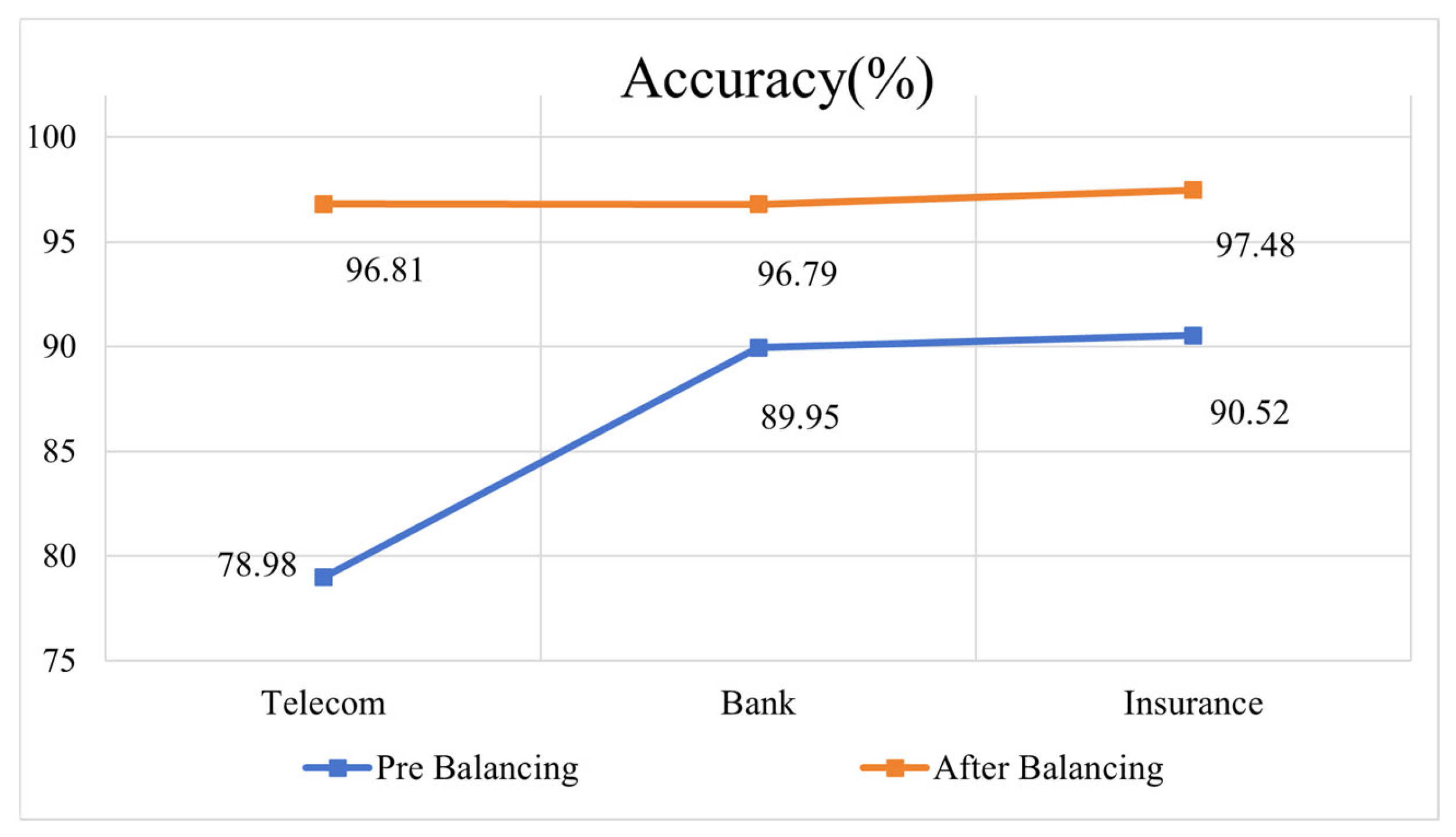
4.5. Impact of SMOTE-ENN on Model Performance

In order to investigate the effect of the category imbalance on our proposed CNN-BiLSTM-FC-CoAttention model, we analyse the performance of the model in four metrics (accuracy, precision, recall and F1-Score) before and after resampling using the SMOTE-ENN. The experimental results are shown in Figure 18, Figure 19, Figure 20 and Figure 21.

The experimental results show that processing the imbalanced dataset by the resampling technique can significantly improve the performance of the model on all the metrics. From the experimental results in Figure 13, it can be seen that on the original dataset without the use of the SMOTE-ENN, the model performs lower in terms of accuracy, especially on the telecom dataset, where the accuracy is only 78.98%. This is due to the fact that the original dataset has fewer churned customers and the model is fitted towards non-churned customers during the training process, resulting in an insufficient predictive power for the sample of churned customers. Whereas, after using the SMOTE-ENN, the accuracy of the model is significantly improved, reaching 96.81% (telecom dataset), 96.79% (bank dataset) and 97.48% (insurance dataset), respectively. It indicates that balancing the dataset by the resampling technique makes the model more effectively learn the features of few classes and thus improves the prediction accuracy. From Figure 14, it can be seen that the precision of the model improves substantially after resampling, especially on the telecom dataset and the insurance dataset, by 36.58% and 35.87%, respectively. It indicates that the use of the SMOTE-ENN can effectively reduce the misjudgement rate of the model for non-churned customers, thus effectively improving the accuracy rate. As can be seen from Figure 15, on the original dataset without the use of the SMOTE-ENN, the recall rate of the model is low, which indicates the poor ability to identify the churn customer samples. The SMOTE-ENN improves the recall of the model by synthesising a few classes and eliminating the noisy data, reaching 97.99% (telecom dataset), 98.59% (bank dataset) and 98.72% (insurance dataset), respectively. The F1-Score, which is the harmonic mean of the precision rate and the recall rate, is able to comprehensively reflect the performance of the model. According to the results in Figure 16, the F1-Score of the models without using resampling techniques are poor, especially on the bank dataset and insurance dataset, which are 55.47% and 56.82%, respectively. Whereas, using the SMOTE-ENN, the F1-Score of the models are significantly improved, reaching 97.15% (telecom dataset), 97.17% (bank dataset) and 97.68%(insurance dataset), respectively. This indicates that the SMOTE-ENN can enable the model to maintain a high precision rate while improving the model’s ability to recognise a small number of classes, thus improving the overall performance of the model.

5. Conclusions

In this study, in order to assist enterprises in identifying churned customers, we propose a novel deep learning model, CNN-BiLSTM-FC-CoAttention, based on one-dimensional convolutional neural networks, bidirectional long and short-term memory networks and coordinate attention mechanisms. The model extracts local and temporal features from customer data through multiple networks in parallel, effectively compensating for the single network’s defect of insufficient feature extraction. In addition, we use the coordinate attention mechanism to enhance the important features of the feature map related to churn behaviour at channel locations and coordinate locations, which further improves the overall performance of the model. We conducted experiments on telecom, banking and insurance datasets. (1) In the hyperparametric experimental section, we performed parameter exploration to select appropriate parameter configurations for the model. (2) In order to compare the performance of the models, we analysed them with traditional machine learning models, ensemble learning models and deep learning models in the comparison experiments section, and the results show that our model outperforms the comparison models in terms of accuracy, precision, recall and F1-value metrics, and demonstrates an excellent prediction performance and generalisation ability. (3) In order to compare the difference and performance of different attention mechanisms in this task, we compared the use of coordinate attention with the use of SENet and CBAM in different metrics, and show the number of parameters, running time and memory consumption of different attention mechanisms, and the results show that the use of different attention mechanisms can improve the prediction performance of the model to varying degrees, but the number of parameters, running time and memory consumption also increase and the memory consumption also increases with them. (4) We verified the importance of each module through ablation experiments, and the synergistic effect of these modules made the model show a superior performance in this study. Then, we discussed the F1 values and confidence intervals of different models and visualised them using error bars, which confirmed the better stability and robustness of the proposed model. In addition, we conducted experiments on the original unbalanced dataset versus the balanced dataset of the model and evaluated the model performance using ROC curves and the area under the curve, which showed that the proposed model had an excellent performance on different datasets and is well adapted to the complex task of churn prediction. (5) We explored the performance of the model before and after using the SMOTE-ENN, and the results confirmed that this resampling technique enables the model to effectively overcome the category imbalance problem.

Since customers in different industries have different behavioural patterns and data distributions, in the future we plan to explore domain adaptation techniques and migration techniques to enhance the model’s ability to learn in different domains. In addition, for our proposed black-box model, we plan to introduce local interpretable techniques or post-interpretable techniques in the future to help decision makers better understand the model’s prediction results. For example, we will combine the Shapley Additive Explanations (SHAP) technique to quantify the contribution of each customer feature to the prediction task and rank and analyse different features by comparing their SHAP values. Since our model uses the attention mechanism, we also plan to observe the feature areas that the model focuses on during the prediction process with the help of attention visualisation techniques and to compare and analyse the model output with the key factors in the real business environment with business experts. Since there are always more retained customers than churned customers in real business scenarios, we plan to further optimise the model architecture or use more advanced resampling techniques in the future to better accommodate the original unbalanced dataset. In addition, we plan to explore more efficient feature extraction methods and lightweight attention mechanisms in the future to reduce model parameters and improve the response speed. Through these measures, we hope to help companies identify potential lost customers in a more timely manner and better maintain customer relationships, so as to maintain an edge in the highly competitive market.