Abstract
This paper addresses the 3D relative localization problem for two unmanned aerial vehicles (UAVs) using a combination of time-of-arrival (TOA) and angle-of-arrival (AOA) measurements across varied flight trajectories. We commenced by examining the problem of relative attitude estimation using only time-of-arrival (TOA) measurements, taking into account a distance-dependent noise model. To address this issue, we constructed a constrained weighted least squares (CWLS) problem and applied semidefinite relaxation (SDR) techniques for its resolution. Furthermore, we extended our analysis to incorporate AOA measurements and scrutinize the Cramer–Rao Lower Bound (CRLB) to illustrate enhanced localization accuracy through TOA-AOA integration compared to TOA alone under stable trajectory conditions. Ultimately, numerical simulations substantiate the efficacy of the proposed methodologies.
1. Introduction
Research on multi-unmanned aerial vehicle (UAV) systems has garnered considerable attention in recent years due to the promising applications of these systems across a multitude of fields, including emergency communication, disaster relief, and power grid detection [1,2,3,4,5,6]. Precise relative localization, which encompasses both position and orientation, is paramount for the cooperative stability of multiple UAVs [7,8,9,10,11], facilitating effective mission execution, collision avoidance, and strategic path planning within UAV swarms.
Traditionally, absolute positioning through global localization methods, such as GPS and wireless sensor networks (WSNs), are employed to indirectly ascertain relative positions among UAVs by providing each UAV’s location within a unified reference frame. The combination of GPS with inertial navigation systems (INSs) has been widely adopted, utilizing techniques such as belief propagation (BP) [12,13,14] or factor graph optimization [15,16] to augment both accuracy and continuity, even in instances where GPS signals are attenuated.
Wireless sensor networks (WSNs) provide an alternative for GPS-denied environments, utilizing time-of-arrival (TOA), angle-of-arrival (AOA), and frequency-of-arrival (FOA) measurements to derive relative positions [17,18,19,20,21,22]. TOA-based methods depend on time delays to estimate inter-node distances, whereas AOA and FOA capitalize on angular and frequency measurements to enhance positioning accuracy. Nevertheless, WSNs necessitate fixed anchors or established infrastructure, constraining their applicability in dynamic or infrastructure-less environments.
Given these constraints, relative pose estimation among UAVs presents an appealing alternative, facilitating a more adaptable and infrastructure-independent approach to uphold stability and coordination within UAV swarms [23,24,25,26,27,28]. By leveraging inter-UAV measurements directly—without the need for external anchors—relative localization provides a resilient solution that can operate effectively in GPS-denied or infrastructure-limited environments. This approach derives positional and orientational information exclusively from inter-UAV measurements, leveraging various sensing modalities, including visual, LiDAR, and radio signal assessments.
Visual and LiDAR-based methods bestow exceptional accuracy for UAV relative localization by delivering intricate spatial information and high resolution [29,30,31]. Vision-based approaches depend on camera sensors to extract and track visual features. However, they frequently necessitate considerable computational resources and are sensitive to environmental factors such as fluctuations in lighting and occlusions [32]. Similarly, LiDAR captures precise depth information through 3D point clouds, providing robustness in various lighting conditions [33]. However, factors such as fog, dust, and rain can scatter or absorb LiDAR signals, impacting performance [34]. Furthermore, LiDAR’s computational and energy demands limit its feasibility for lightweight UAVs, making both methods challenging for real-time applications within dynamic environments.
Radio-based methods present considerable advantages for UAV relative localization, particularly in dynamic, anchor-free environments where flexibility and minimal computational demands are crucial. In an inter-UAV range measurement system, two UAVs mutually exchange distance measurements to accumulate sufficient information for relative localization. This arrangement is straightforward and practical for dynamic, anchor-free contexts, rendering it a significant area of research.
Considering these advantages, various approaches have been proposed to tackle the relative pose estimation dilemma utilizing radio-based measurements. In particular, the constraints on the rotation matrix, such as the orthonormality condition , must be carefully considered to ensure valid solutions in relative pose estimation. For instance, ref. [27] formulates a constrained weighted least squares (CWLS) problem that disregards noise terms, transforming it into a semidefinite programming (SDP) problem solved through semidefinite relaxation (SDR). Building on this foundation, ref. [21] integrates quaternions into the framework and employs quadratic constrained quadratic programming (QCQP) to enhance estimation accuracy.
Further advancing the discourse, ref. [24] incorporates inertial measurement unit (IMU) errors into the model, devising a motion-based framework to account for cumulative error effects. This methodology also utilizes SDR for the solution and is validated through empirical experiments, underscoring its robustness, while other studies, such as [35], propose deterministic schemes with global exponential stability or robust fusion approaches [36] to address challenges like non-line-of-sight (NLOS) errors in complex environments.
Although effective, TOA-only methods may struggle to achieve high localization precision in certain scenarios. Inspired by recent advancements in visual-based [29,30,31] and AOA-based [20,21] localization techniques, we integrate AOA measurements with TOA. Advances in antenna technology [37,38,39] now enable compact angle measurement arrays on UAVs, making joint TOA-AOA localization feasible. By combining distance and angular information, our approach aims to enhance the precision and adaptability of inter-UAV relative pose estimation.
Despite recent advances, the challenge of joint TOA-AOA relative localization remains unaddressed, particularly in dynamic UAV environments. The specific influence of UAV flight trajectories on AOA measurements—namely, the variations in azimuth and elevation angles along different paths—has yet to be thoroughly investigated in the context of relative localization accuracy [28]. Understanding these angular variations is vital, as they directly affect the stability and precision of inter-UAV localization in practical applications. This highlights the pressing need for research into the trajectory-dependent factors shaping TOA-AOA localization, underscoring the potential for achieving more accurate and resilient UAV operations through optimized measurement integration.
In this paper, we develop an optimal joint relative pose estimation framework that leverages TOA and AOA measurements to enhance 3D relative localization accuracy between UAVs significantly. By integrating distance and angular data, our method transcends the limitations of conventional approaches that rely solely on distance, providing a more resilient solution for UAV operations in dynamic, infrastructure-constrained environments. Utilizing TOA and AOA information within an SDP framework, we address the inherent non-convexity of the pose estimation problem, transforming it into a convex optimization task through the application of SDR. Furthermore, we conduct a comprehensive Cramer–Rao Lower Bound (CRLB) analysis to evaluate the theoretical accuracy bounds of the proposed method across diverse noise levels and trajectory scenarios.
Our main contributions are as follows:
- The CRLB under a distance-dependent noise model for UAV relative pose estimation is derived, providing a theoretical benchmark for the achievable accuracy of TOA-AOA measurements.
- A novel joint TOA-AOA formulation for relative pose estimation is developed, combining distance and angle measurements to enhance localization accuracy in anchor-free environments.
- An efficient SDR estimator is devised to handle the nonlinearity and orthogonality constraints, and its effectiveness is demonstrated through comprehensive simulations under various noise and trajectory conditions.
The remainder of this paper is organized into the following sections. Section 2 introduces the problem formulation for 3D relative pose estimation between UAVs based on TOA and AOA measurements. Section 3 presents the SDR method for addressing the relative localization problem, initially applying it to TOA-only measurements and extending it to the combined TOA-AOA model. Section 4 derives the CRLB and analyzes its implications for localization accuracy. Section 5 provides numerical simulations to evaluate the performance of the proposed methods under various noise conditions and flight trajectories. This paper is concluded in Section 6.
In accordance with standard conventions, a bold lowercase letter (a) denotes a column vector, while a bold uppercase letter (A) signifies a matrix. The symbols and are used to denote matrix inversion and transpose operations, respectively. The notation refers to the norm of a vector. The expression represents the i-th element of the vector , and denotes the sub-vector of that includes elements from the i-th to the j-th position. Similarly, indicates the -th element of the matrix . The symbol stands for the identity matrix. The operation denotes the Kronecker product of matrices and . The functions and compute the trace and the rank of matrix , respectively. For a square matrix , the operation results in a vector formed by stacking the columns of one beneath the other, such that for .
2. Problem Formulation
In this section, we introduce the system model of two drones that achieve relative pose estimation using inter-drone distance measurement in 3D space.
System Model
Consider two drones, UAV 1 and UAV 2, operating in a 3D environment. UAV 1 serves as the reference with its position in the global coordinate system represented as . UAV 2, whose position is to be determined, is defined within its local body coordinate system as . To map the local coordinate system of UAV 2 to the global frame, we apply a coordinate transformation consisting of a rotation vector and a translation vector .
To convert the rotation vector into a rotation matrix , we utilize the exponential map from the Lie algebra so(3) to the Lie group SO(3) [28]. The orthogonality constraints, specifically and arise from the structural properties of rotation matrices, ensuring that represents a valid rotation in three-dimensional space.
The rotation matrix is computed as
where is the skew-symmetric matrix associated with the rotation vector . The exponential of this skew-symmetric matrix yields the rotation matrix required for the coordinate transformation [28]. The skew-symmetric matrix is defined as
Thus, the position of UAV 2 in the global coordinate system can be represented as
To achieve the relative localization of UAV 2 with respect to UAV 1, we utilize both TOA and AOA measurements. It is assumed that UAV 2 can transmit a signal containing its local coordinate information , which UAV 1 then receives. Upon reception, UAV 1 measures the distance to UAV 2 through TOA and estimates the relative angle through AOA. This signal processing provides UAV 1 with the range, angle, and UAV 2’s local coordinate data, enabling the transformation of UAV 2’s local position into the global frame and achieving precise relative localization. As illustrated in Figure 1.
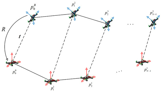
Figure 1.
Scenario of UAV relative localization estimation.
The two UAVs undergo a total of N movements, each characterized by uniform rectilinear motion with a consistent time interval, , between movements. This ensures constant velocities, and , for UAVs 1 and 2, respectively, without any acceleration. The position updates for the UAVs are given by
where and denote the positions at the n-th movement step. The velocities of both UAVs at all movement steps are compactly represented in the column vector . We assume that the vector is error-free, meaning that the recorded velocities are accurate and do not contain any measurement inaccuracies. This assumption holds reliably over short time intervals.
Assume that the signal transmitted from UAV 2 contains a pilot header, and the clocks of the two UAVs are perfectly synchronized. Based on correlation computations, the range measurement can be obtained, making TOA feasible. For the n-th measurement, where , the distance between the two UAVs is given by
where the actual distance between UAV 1 and 2 is denoted by . The distances between UAV 1 and UAV 2 at all movement steps are compactly represented in the column vector .
The measurement noise, characterized by a normal distribution with a mean of zero and a variance of , is represented by . It is noteworthy to mention that the noise covariance is proportional to the distance. This is due to the fact that the ranging is based on communication signals, and as the distance increases, the signal-to-noise ratio (SNR) decreases, leading to a higher noise variance. Following the approach in [40,41], we assume that the relationship between the variance and the distance satisfies the equation
where and are parameters that define the scaling and power–law relationship between the noise variance and the distance, respectively. is the reference distance, which we assume to be 1 m, is 0.01, and is equal to 2.
To streamline the notation, we compile the noise elements into a single vector , which is transposed as . According to the distance-related noise model, the covariance matrix for the noise vector is given by
where each element on the diagonal of corresponds to the variance of the noise for the respective distance measurement .
Given only ranging measurements, our task is to solve for
The ranging function is a typical nonlinear and non-convex function due to the presence of Euclidean norms in the formulation. This inherent non-convexity significantly increases the complexity of the problem, making it challenging to find a global optimum.
For angular measurements, we denote as the unit vector representing the true angle between UAV 2 and UAV 1, as measured by UAV 1 in the current body frame coordinate system [30,42]. This value is defined as follows:
where represents the true distance at the current time instant. The noisy measurement of the angle can be expressed as
Here, is a rotation matrix that also satisfies the SO(3) group. This definition is chosen to ensure that the vector maintains its characteristic as a unit vector. The unit vectors for the angular measurements between UAV 1 and UAV 2 at all movement steps are compactly represented in the column vector .
When the angular measurement noise is relatively small, we can approximate the rotation matrix as , where is an anti-symmetric matrix [18,19,20]. The specific form of is given by
Here, , , and represent the small angular perturbations around the respective axes. Defining , we assume that they follow a normal distribution with the covariance matrix being a diagonal matrix, denoted as . In particular, we set . This choice is made to facilitate a comparative analysis of the extent to which the performance of ranging measurements is enhanced under varying levels of angular noise.
Similar to a ranging-only scenario, when angular measurements are available, our task is to solve for
3. SDR Method for Relative Localization
In this section, we first develop a TOA-based model for relative localization and then extend it to incorporate AOA measurements. Through semidefinite relaxation, we transform the problem into a solvable convex form to estimate the rotation matrix and translation vector.
3.1. SDR Method Using TOA Only
We commence our analysis with the TOA measurement model, as outlined in Equation (5). This particular issue has been investigated in prior research, as documented by [27].
By transferring to the left side and squaring both sides of the equation, we arrive at the simplified expression:
The squared second-order noise contribution, , is excluded from consideration since it is considered trivial in comparison to the first-order noise term, given the premise that noise levels are minimal.
By defining as the unknown variable, we can rewrite Equation (15) into a more compact matrix form:
where for , we have
Building upon Equation (16) and considering the SO(3) constraint for the rotation matrix , we can pose the CWLS problem as follows:
The weighting matrix is defined as the inverse of :
Let us begin by considering the structure of the constraint Equation (21b). The constraint implies that the rotation matrix must be a member of the special orthogonal group, which requires that and . For the purpose of our derivation, we initially disregard the determinant constraint.
leads to a total of six constraint equations. Additionally, considering the nonlinear terms involving and within the vector , we can further augment the number of constraint equations. According to the derivation presented by [27], it is sufficient to employ a total of ten constraint equations to solve the problem. This result is substantiated by [28], which demonstrates that the constraint space formed by these ten equations is sufficiently tight.
By using the method of increasing the order, known as the higher-order lifting function of the vector , we define
The ten constraint equations can be represented using inner products (dot products) as follows:
where is a symmetric matrix. Each corresponds to the construction of a different constraint equation, with representing the constant associated with each of the ten constraints.
We will employ a sparse matrix notation to construct the matrix . Specifically, this construction involves identifying the row and column indices of the non-zero elements along with their corresponding values. In the case of , its sparse representation comprises M non-zero entries, with the set of row indices denoted as , the set of column indices as , and the non-zero values at . Consequently, can be succinctly expressed as [26].
The representations of these ten matrices are as follows:
The ultimate expression for Formula (21a) can be cast by setting
which allows us to reformulate it as
The rank constraint makes the problem inherently non-convex. To make the problem solvable, we apply the SDR technique by relaxing this constraint and later compensating for it. By eliminating the rank constraint, the problem is converted into an SDP issue, which can be effectively tackled using the CVX toolbox. The matrix , specified in Equation (22), remains undetermined due to its reliance on the actual values. To facilitate a feasible approach, we initialize as the identity matrix and proceed to solve the problem presented in Equation (27) for an initial approximation. Subsequently, this preliminary estimate is employed to refine the weighting matrix. Following this adjustment, we re-solve the problem in Equation (27) to arrive at the ultimate solution.
If the SDP solution is tight enough, then we should have . We can use the Singular Value Decomposition (SVD) to obtain and extract and . Since we relaxed the constraint earlier, we need to compensate for this here. After obtaining , we seek by solving
where represents the Frobenius norm. We can use the Procrustes algorithm [27], specifically the SVD-based method, to find the solution as follows:
After the optimization process, the final results that we obtain are the rotation matrix and the translation vector . To convert the rotation matrix back into a rotation vector using Lie algebra, we apply the logarithmic map [28]. The rotation vector can be obtained from the rotation matrix using the following relationship:
where the operation denotes the conversion of a skew-symmetric matrix back into a vector. We list the steps of SDR-TOA in Algorithm 1.
| Algorithm 1 SDR-TOA. |
| Data: range measurement vector , UAV speed vector , UAV initial positions and , noise related parameters and Result: relative pose estimation and 1: Compute and using (17) and (18) respectively; 2: Initialize ; 3: Compute using (26); 4: Construct constraints equations using (25); 5: Solve by optimizing (27); 6: Extract and from ; 7: Compute using (29) and (30); 8: Update using (22); 9: Solve by optimizing (27) with updated ; 10: Repeat 6–7; |
3.2. SDR Method Using TOA and AOA Measurements
In this section, we will introduce an SDR approach for the TOA-AOA relative localization issue. First, by reformulating Equation (9), we obtain the following:
Utilizing Equation (11), we obtain the following:
Omitting the second-order noise term , and using Equations (14) and (32), we have, for , the following:
By defining , we can construct a CWLS problem similar to Equation (16) as follows:
where for , we have
The covariance matrix of the noise vector , denoted as , can be expressed as . For each , the corresponding block is given by , where and are the covariance matrices for the noise associated with angle measurement and distance measurement, respectively. The weighting matrix is defined as
Similarly, define as
and let be defined as
Finally, we arrive at a formula similar to (27), but it is important to note that at this point, contains only the linear terms of and , and does not include the nonlinear terms such as or . Consequently, the constraint equations are limited to the six equations involving the rotation matrix, which are . Thus, we can formulate the following semidefinite programming (SDP) problem:
By relaxing the rank constraint, we ultimately formulate a solvable SDP problem. Similar to the TOA-only scenario, the obtained solution can also be decomposed using SVD to yield estimates of the rotation matrix and translation vector . Utilizing the Procrustes algorithm in conjunction with the Log map, we ultimately derive the estimated rotation vector and the translation vector through the combined TOA-AOA estimation process. We list the steps of SDR-TOA in Algorithm 2 below.
| Algorithm 2 SDR-TOA-AOA. |
| Data: range measurement vector , angular measurement vector , UAV speed vector , UAV initial positions and , noise related parameters and Result: relative pose estimation and 1: Compute and using (35) and (36) respectively; 2: Initialize ; 3: Compute using (39); 4:bConstruct constraints equations using (25); 5: Solve by optimizing (27); 6: Extract and from ; 7: Compute using (29) and (30); 8: Update using (37); 9: Solve by optimizing (41) with updated ; 10: Repeat 6–7; |
4. Performance Analysis
In this section, we derive the CRLB to assess the impact of AOA measurements on localization accuracy, highlighting their effectiveness in enhancing estimation precision.
4.1. CRLB Analysis for TOA Measurements Only
In this section, we proceed to derive the CRLB for relative pose estimation when only TOA-based range measurements are available.
Firstly, we define the vector of parameters to be estimated as , where and represent the rotation vectors and translation vectors, respectively. We can then construct the likelihood function for the range measurements as follows:
Here, denotes the vector of range measurements, is the vector of real range measurements, is the covariance matrix of the range measurement errors, and N is the number of measurements.
When the covariance of the measurements is correlated with the variables to be estimated, we can express the CRLB and the Fisher information matrix in the following form [40,41]:
where the i-th row of , denoted as , could be expressed as follows:
The term can be expressed as
4.2. CRLB Analysis for TOA-AOA Measurements
Next, we proceed to derive the CRLB for relative pose estimation when both TOA range measurements and AOA angular measurements are available.
Considering that ranging and angle measurements are independent of each other, the joint likelihood function under the TOA-AOA scenario can be expressed as
Utilizing Formulas (10), (11), and (32), we can express the angular measurement error in the form of an additive domain as where denotes the measured angle and denotes the true angle for the i-th measurement. To further compute the covariance of the angular measurement error, , it can be represented as follows:
Since the noise in angle measurement is indirectly dependent of the range as , the CRLB and the Fisher information matrix under TOA-AOA measurements could be formulated as
By substituting Equation (9), we can express the term as follows:
Considering that the is necessarily positive semidefinite, given that the FIM is a semidefinite positive matrix, the CRLB for the combined measurement case satisfies the inequality
indicating that the inclusion of additional AOA measurements lead to a lower bound on the variance of the estimator for , thereby enhancing estimation accuracy compared to using TOA measurements alone.
The influence of and on the CRLB exhibits distinct characteristics due to their roles in the measurement process. , as the covariance matrix of range measurements, directly impacts , which naturally reflects the uncertainty in the distance measurements. This influence is further complicated because , the covariance matrix of angular measurements, is indirectly related to through a proportional factor , representing the dependency between the variances of range and angular noise. Consequently, changes in also indirectly affect , thereby influencing . These interdependencies highlight the complex interactions between range and angular measurement uncertainties and their combined effects on the overall CRLB.
5. Numerical Experiments
We conducted simulations to evaluate the performance of the proposed methods (denoted as “SDR-TOA” and “SDR-TOA-AOA”). In these simulations, the SDR-TOA-RAW [20] is used as benchmark. The MATLAB toolbox CVX was employed to address the SDP issues, utilizing SDPT3 as the designated solver. We used the root mean squared error (RMSE) as the performance metric, defined as
where and denote the real value of rotation angle and translation vectors, while and represent the estimate of the true value during the i-th iteration of the Monte Carlo (MC) simulation for the j-th setup, with L and MC representing the number of configurations and MC runs, respectively.
5.1. Simulation Configuration
The TOA and AOA measurements were generated using models (5) and (9), respectively. We set the number of MC runs to 1000, with 4 distinct flight trajectories (configurations) within a 100 m × 100 m × 100 m 3D space. The rotation angle was fixed at rad. The four trajectories, shown in Figure 2, include parallel paths, intersecting paths, spiral paths with increasing altitude, and circular paths in opposite directions. The selected flight path scenarios were carefully designed to evaluate the practical limitations and performance of the proposed method under varying motion patterns.
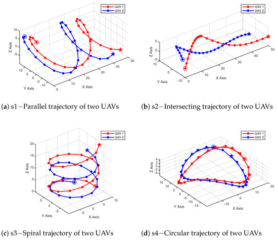
Figure 2.
Four trajectories of two UAVs.
Specifically, trajectories s2 and s4 were chosen to compare the differences between parallel and opposing (intersecting) flight paths, highlighting the effect of relative motion direction on localization accuracy. On the other hand, trajectories s1 and s3 were selected to investigate the impact of AOA measurements under scenarios with similar TOA conditions. In particular, s1 focuses on angle measurements concentrated in the XY-plane, while s3 emphasizes angle measurements in the Z-direction. This comparison allowed us to analyze the influence of angular diversity on the relative pose estimation results.
The red line represents the trajectory of UAV 1, while the blue line corresponds to that of UAV 2. The trajectories are designated as s1, s2, s3, and s4. The starting points of UAVs are marked with circles, while the endpoints are denoted by stars.
For each configuration, 50 groups of range and angle measurements were taken, with only the first 25 used for TOA and TOA-AOA comparisons unless otherwise specified. The simulation generated noise-free range and angle measurements, and Gaussian noise was subsequently added to model realistic sensor errors. The TOA noises followed a zero-mean Gaussian distribution with covariance , while the AOA noises followed a zero-mean Gaussian distribution with covariance , where denotes the ratio between AOA and TOA noise levels. This setup ensures that the influence of measurement noise and the integration of AOA measurements can be effectively analyzed under constrained conditions.
We assumed a measurement frequency of 5 Hz for both range and angle, meaning that a range and angle measurement was completed every 0.2 s. Additionally, we assumed that the maximum speed of the UAV would not exceed 10 m/s. Pose estimation was performed after collecting the required N number of range and angle measurements.
5.2. Performance Comparison of Measurement Noise Variance
Our proposed algorithm consistently outperforms the SDR-TOA-RAW [20] benchmark across all trajectories, as seen in Figure 3. This superior performance is due to our algorithm’s comprehensive consideration of noise and distance-related models. By integrating AOA measurements alongside TOA, our approach significantly enhances the observability of the system, leading to improved estimation accuracy.
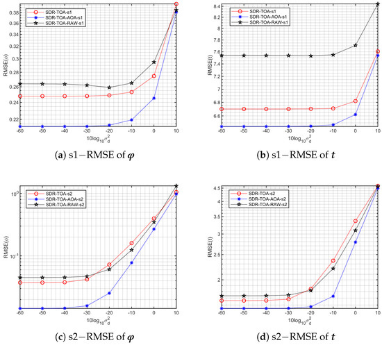
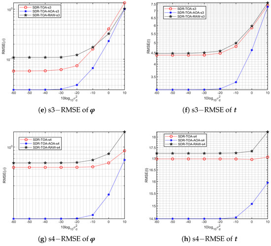
Figure 3.
Acomparison of the influence of noise level on the SDP under different flight trajectories.
The four trajectories exhibit distinct differences in localization accuracy due to variations in relative distance and measurement stability. As shown in Figure 3g,h, trajectory s4 consistently yields the highest localization error across all noise levels, primarily because of its significant fluctuations in relative position, elevation, and azimuth angles, which reduce measurement stability and amplify errors. In contrast, trajectories s2 and s3 demonstrate better localization performance due to more stable relative distances, which enhance the quality of ranging information and improve overall accuracy, as shown in Figure 3c–f.
Among these, trajectory s2 achieves the best accuracy. By comparing the TOA-only (SDR-TOA and SDR-TOA-RAW) and TOA-AOA results in Figure 3, it is evident that the inclusion of AOA measurements significantly enhances accuracy across all trajectories. For instance, with −20 dB noise (corresponding to a 0.1 m standard deviation in range measurements), the rotational vector estimation error for s2 improves from 0.085 to 0.026, reflecting a improvement, as shown in Figure 3c. Similarly, for s3, the rotational vector error decreases from 0.12 to 0.031, reflecting a improvement, as shown in Figure 3e. The translational vector estimates are relatively stable, with s2 improving from 0.019 m to 0.017 m and s3 from 0.045 m to 0.032 m, as shown in Figure 3d,f, respectively. These findings highlight the advantage of leveraging stable relative positions in trajectories to fully exploit the benefits of AOA.
Each trajectory also displays distinct sensitivity to noise. As shown in Figure 3a,b,g,h, trajectories s1 and s4 exhibit smaller error increases as noise levels rise, indicating greater robustness to noise. In contrast, s2 and s3 show sharper error growth at higher noise levels. This suggests that while s2 and s3 substantially benefit from AOA at lower noise levels, they are more susceptible to error amplification as noise increases. Collectively, these findings underscore the importance of both stable measurement geometry and noise robustness in optimizing UAV relative localization.
5.3. Performance Comparison of TOA and AOA Measurement Noise Ratio
In this subsection, we investigate the effect of increasing the AOA noise ratio on localization accuracy across different trajectories. Our goal is to understand how the addition of AOA measurements impacts the performance under varying noise conditions.
It is evident that the influence of on TOA-AOA performance is highly trajectory-dependent. As illustrated in Figure 4, for s2 and s3, when exceeds 8, the TOA-AOA method performs worse than the TOA-only method. It occurs because the inaccuracies in AOA estimation at high noise levels deteriorate the overall localization accuracy. Furthermore, with regard to rotational vector estimation, Figure 4a reveals that s2 performs worse than s3 at higher values, although s2 still outperforms s3 in translational vector estimation.
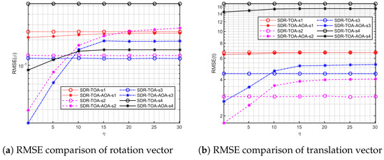
Figure 4.
A comparison of the influence of noise levels on the SDR TOA and TOA-AOA methods under four different flight trajectories.
In contrast, trajectories s1 and s4 show relatively stable localization performance as increases. This aligns with our findings from the first experiment regarding noise sensitivity, where s1 and s4 exhibited stronger noise robustness, albeit at the cost of lower baseline accuracy. Thus, these results confirm that while trajectories with stable measurement conditions (like s2 and s3) benefit more from AOA at lower noise levels, they are also more sensitive to increases in AOA noise, whereas s1 and s4 demonstrate better resilience to noise fluctuations but with lower overall accuracy.
While the inclusion of AOA measurements generally enhances localization accuracy, as shown in Figure 4, the improvement becomes less significant when AOA noise levels are relatively high. In such cases, the information provided by angle measurements may contribute less to the overall accuracy, making the additional computational effort for processing AOA less effective. In practical applications, this trade-off should be carefully considered. When AOA noise is substantial, it may be worth evaluating whether incorporating AOA measurements is beneficial or if a TOA-only approach could achieve comparable performance with reduced complexity.
5.4. Performance Comparison of Number of Measurements
We investigated the influence of the number of observations on relative positioning accuracy. To conduct this research, we set to 0.1 m and to 0.3, gradually increasing the number of observations N from 25 to 50. In this process, we used CRLB as an evaluation metric. It can be seen clearly from Figure 5 that this result is consistent with the results of the previous two experiments: s2 corresponds to the best positioning effect, while s4 shows the worst positioning performance. However, it is worth noting that regardless of which flight trajectory, the localization accuracy has shown a significant improvement trend as the number of observations increase. This means that more observations can indeed bring better localization accuracy.
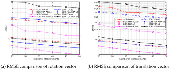
Figure 5.
A comparison of the influence of number of measurements on the SDR TOA and TOA-AOA methods under four different flight trajectories.
6. Conclusions
This study addresses the 3D relative localization problem for UAVs using a hybrid approach of TOA and AOA measurements. We first established baseline localization performance using TOA-only measurements under varied noise conditions, formulating the problem as a CWLS model to estimate the relative position and orientation of the UAVs. To manage the non-convexity and orthogonality constraints of the rotation matrix, we applied SDR to transform the model into a convex semidefinite program. Expanding our analysis to include AOA measurements, we demonstrated that integrating TOA with AOA significantly enhances localization accuracy, especially for stable flight trajectories. Through CRLB analysis and extensive numerical simulations, we validated that the proposed TOA-AOA approach outperforms TOA-only localization across diverse trajectory configurations, providing a robust solution for relative UAV localization.
The proposed algorithm can be applied to practical scenarios such as UWB-based ranging systems and Bluetooth-based AOA measurement systems. By leveraging both TOA and AOA measurements, our approach highlights the importance of UAV trajectory selection in achieving accurate relative localization. Specifically, optimizing flight trajectories can significantly enhance localization performance, which is particularly valuable for UAV swarm operations in GPS-denied environments. Additionally, the flexibility of our method allows for integration with other sensing modalities, such as IMUs, cameras, or LiDARs, enabling robust multi-sensor fusion solutions for real-world UAV applications.
Author Contributions
Conceptualization, X.D. and D.L.; Methodology, J.T.; Software, T.C.; Validation, J.T.; Formal analysis, Q.J. All authors have read and agreed to the published version of the manuscript.
Funding
This work was supported in part by the National Key Research and Development Program of China under Grant 2023YFC3305904, in part by the National Natural Scientific Foundation of China under Grant 62301049, and in part by the Natural Science Foundation of Shandong Province of China under Grant ZR2024QF028.
Data Availability Statement
The original contributions presented in this study are included in the article. Further inquiries can be directed to the corresponding author.
Conflicts of Interest
The authors declare no conflicts of interest.
References
- Ye, X.; Song, F.; Zhang, Z.; Zeng, Q. A Review of Small UAV Navigation System Based on Multisource Sensor Fusion. IEEE Sens. J. 2023, 23, 18926–18948. [Google Scholar] [CrossRef]
- Wang, S.; Wang, Y.; Bai, X.; Li, D. Communication Efficient, Distributed Relative State Estimation in UAV Networks. IEEE J. Sel. Areas Commun. 2023, 41, 1151–1166. [Google Scholar] [CrossRef]
- Pan, J.; Ye, N.; Yu, H.; Hong, T.; Al-Rubaye, S.; Mumtaz, S.; Al-Dulaimi, A.; Chih-Lin, I. AI-Driven Blind Signature Classification for IoT Connectivity: A Deep Learning Approach. IEEE Trans. Wirel. Commun. 2022, 21, 6033–6047. [Google Scholar] [CrossRef]
- Chen, R.; Yang, B.; Zhang, W. Distributed and collaborative localization for swarming UAVs. IEEE Internet Things J. 2020, 8, 5062–5074. [Google Scholar] [CrossRef]
- Ding, X.; Zhou, K.; Li, G.; Yang, K.; Gao, X.; Yuan, J.; An, J. Customized Joint Blind Frame Synchronization and Decoding Methods for Analog LDPC Decoder. IEEE Trans. Commun. 2024, 72, 756–770. [Google Scholar] [CrossRef]
- Ding, X.; Zhang, Y.; Li, J.; Mao, B.; Guo, Y.; Li, G. A feasibility study of multi-mode intelligent fusion medical data transmission technology of industrial Internet of Things combined with medical Internet of Things. Internet Things 2023, 21, 100689. [Google Scholar] [CrossRef]
- Gu, X.; Zheng, C.; Li, Z.; Zhou, G.; Zhou, H.; Zhao, L. Cooperative Localization for UAV Systems From the Perspective of Physical Clock Synchronization. IEEE J. Sel. Areas Commun. 2024, 42, 21–33. [Google Scholar] [CrossRef]
- Hua, B.; Ni, H.; Zhu, Q.; Wang, C.X.; Zhou, T.; Mao, K.; Bao, J.; Zhang, X. Channel Modeling for UAV-to-Ground Communications with Posture Variation and Fuselage Scattering Effect. IEEE Trans. Commun. 2023, 71, 3103–3116. [Google Scholar] [CrossRef]
- Shi, M.; Yang, K.; Niyato, D.; Yuan, H.; Zhou, H.; Xu, Z. The Meta Distribution of SINR in UAV-Assisted Cellular Networks. IEEE Trans. Commun. 2023, 71, 1193–1206. [Google Scholar] [CrossRef]
- You, K.; Chen, Q.; Xie, P.; Song, S. Range-based coordinate alignment for cooperative mobile sensor network localization. IEEE Trans. Control Netw. Syst. 2020, 7, 1379–1390. [Google Scholar] [CrossRef]
- Wu, X.; Qi, H. Motion Parameter Estimation for Mobile Sources Using Semidefinite Programming. IEEE Trans. Mob. Comput. 2023, 22, 1066–1080. [Google Scholar] [CrossRef]
- Zhang, Y.; Chen, L.; Chen, X.; Wang, W. A Low-Complexity Soft Localization Algorithm Based on Expectation Propagation. IEEE Commun. Lett. 2023, 27, 2958–2962. [Google Scholar] [CrossRef]
- Li, X.; Wu, Z.; Shen, Z.; Xu, Z.; Li, X.; Li, S.; Han, J. An Indoor and Outdoor Seamless Positioning System for Low-Cost UGV Using PPP/INS/UWB Tightly Coupled Integration. IEEE Sens. J. 2023, 23, 24895–24906. [Google Scholar] [CrossRef]
- Cao, C.; Zhu, Y.; Zhao, L.; Sun, D.; Liu, Z.; Lian, Y. An Accurate Positioning Method Based on Time-Division Strategy for Indoor Moving Target. IEEE Trans. Instrum. Meas. 2023, 72, 1–12. [Google Scholar] [CrossRef]
- Singh, A.; Verma, S. Graph Laplacian Regularization with Procrustes Analysis for Sensor Node Localization. IEEE Sens. J. 2017, 17, 5367–5376. [Google Scholar] [CrossRef]
- Fan, T.; Murphey, T.D. Majorization Minimization Methods for Distributed Pose Graph Optimization. IEEE Trans. Robot. 2024, 40, 22–42. [Google Scholar] [CrossRef]
- Chepuri, S.P.; Leus, G.; van der Veen, A.J. Rigid body localization using sensor networks. IEEE Trans. Signal Process. 2014, 62, 4911–4924. [Google Scholar] [CrossRef]
- Wu, X.; Lin, Q.; Qi, H. Cooperative multiple rigid body localization via semidefinite relaxation using range measurements. IEEE Trans. Signal Process. 2022, 70, 4788–4803. [Google Scholar] [CrossRef]
- Wang, Y.; Wang, G.; Chen, S.; Ho, K.; Huang, L. An investigation and solution of angle based rigid body localization. IEEE Trans. Signal Process. 2020, 68, 5457–5472. [Google Scholar] [CrossRef]
- Dong, X.; Wang, G.; Ho, K.C.; Huang, L. Rigid Body Localization in Unsynchronized Sensor Networks: Analysis and Solution. IEEE Trans. Wirel. Commun. 2024, 23, 2901–2916. [Google Scholar] [CrossRef]
- Li, B.; Wang, X. Rigid body localization and environment sensing with 5G millimeter wave MIMO. In Proceedings of the 2021 IEEE 94th Vehicular Technology Conference (VTC2021-Fall), Norman, OK, USA, 27–30 September 2021; pp. 1–5. [Google Scholar]
- Meng, X.; Li, Y.; Wu, Z.; Hong, S.; Chang, S. A semidefinite relaxation approach for mobile target localization based on TOA and Doppler frequency shift measurements. IEEE Sens. J. 2023, 23, 16051–16057. [Google Scholar] [CrossRef]
- Yu, Q.; Wang, Y.; Shen, Y.; Shi, X. Cooperative Multi-Rigid-Body Localization in Wireless Sensor Networks Using Range and Doppler Measurements. IEEE Internet Things J. 2023, 10, 22748–22763. [Google Scholar] [CrossRef]
- Wang, Y.; Lin, M.; Xie, X.; Gao, Y.; Deng, F.; Lam, T.L. Asymptotically Efficient Estimator for Range-Based Robot Relative Localization. IEEE/ASME Trans. Mechatron. 2023, 28, 3525–3536. [Google Scholar] [CrossRef]
- Mao, K.; Zhu, Q.; Qiu, Y.; Liu, X.; Song, M.; Fan, W.; Kokkeler, A.B.J.; Miao, Y. A UAV-Aided Real-Time Channel Sounder for Highly Dynamic Nonstationary A2G Scenarios. IEEE Trans. Instrum. Meas. 2023, 72, 6504515. [Google Scholar] [CrossRef]
- Li, M.; Lam, T.L.; Sun, Z. 3-D Inter-Robot Relative Localization via Semidefinite Optimization. IEEE Robot. Autom. Lett. 2022, 7, 10081–10088. [Google Scholar] [CrossRef]
- Jiang, B.; Anderson, B.D.; Hmam, H. 3-D relative localization of mobile systems using distance-only measurements via semidefinite optimization. IEEE Trans. Aerosp. Electron. Syst. 2019, 56, 1903–1916. [Google Scholar] [CrossRef]
- Nguyen, T.H.; Xie, L. Relative transformation estimation based on fusion of odometry and UWB ranging data. IEEE Trans. Robot. 2023, 39, 2861–2877. [Google Scholar] [CrossRef]
- Xunt, Z.; Huang, J.; Li, Z.; Ying, Z.; Wang, Y.; Xu, C.; Gao, F.; Cao, Y. CREPES: Cooperative RElative Pose Estimation System. In Proceedings of the 2023 IEEE/RSJ International Conference on Intelligent Robots and Systems (IROS), Detroit, MI, USA, 1–5 October 2023; pp. 5274–5281. [Google Scholar]
- Wang, Y.; Wen, X.; Yin, L.; Xu, C.; Cao, Y.; Gao, F. Certifiably Optimal Mutual Localization with Anonymous Bearing Measurements. IEEE Robot. Autom. Lett. 2022, 7, 9374–9381. [Google Scholar] [CrossRef]
- Wang, Y.; Wen, X.; Cao, Y.; Xu, C.; Gao, F. Bearing-Based Relative Localization for Robotic Swarm with Partially Mutual Observations. IEEE Robot. Autom. Lett. 2023, 8, 2142–2149. [Google Scholar] [CrossRef]
- Zhang, H.; Wang, D.; Huo, J. Mounting Misalignment and Time Offset Self-Calibration Online Optimization Method for Vehicular Visual-Inertial-Wheel Odometer System. IEEE Trans. Instrum. Meas. 2024, 73, 1–13. [Google Scholar] [CrossRef]
- Wang, J.; Zhu, Q.; Lin, Z.; Wu, Q.; Huang, Y.; Cai, X.; Zhong, W.; Zhao, Y. Sparse Bayesian Learning-Based 3-D Radio Environment Map Construction—Sampling Optimization, Scenario-Dependent Dictionary Construction, and Sparse Recovery. IEEE Trans. Cogn. Commun. Netw. 2024, 10, 80–93. [Google Scholar] [CrossRef]
- Gao, J.; Sha, J.; Li, H.; Wang, Y. A Robust and Fast GNSS-Inertial-LiDAR Odometry with INS-Centric Multiple Modalities by IESKF. IEEE Trans. Instrum. Meas. 2024, 73, 1–12. [Google Scholar] [CrossRef]
- Garraffa, G.; Sferlazza, A.; D’ippolito, F.; Alonge, F. Localization Based on Parallel Robots Kinematics As an Alternative to Trilateration. IEEE Trans. Ind. Electron. 2022, 69, 999–1010. [Google Scholar] [CrossRef]
- Liu, J.; Zhang, L.; Xu, J.; Shi, J. Dynamic Feasible Region-Based IMU/UWB Fusion Method for Indoor Positioning. IEEE Sens. J. 2024, 24, 21447–21457. [Google Scholar] [CrossRef]
- Gong, Y.; Zhao, H.; Hu, K.; Lu, Q.; Shen, Y. A Multipath-Aided Localization Method for MIMO-OFDM Systems via Tensor Decomposition. IEEE Wirel. Commun. Lett. 2022, 11, 1225–1228. [Google Scholar] [CrossRef]
- Zhao, H.; Zhang, N.; Shen, Y. Beamspace Direct Localization for Large-Scale Antenna Array Systems. IEEE Trans. Signal Process. 2020, 68, 3529–3544. [Google Scholar] [CrossRef]
- Pöhlmann, R.; Zhang, S.; Staudinger, E.; Dammann, A.; Hoeher, P.A. Simultaneous Localization and Calibration for Cooperative Radio Navigation. IEEE Trans. Wirel. Commun. 2022, 21, 6195–6210. [Google Scholar] [CrossRef]
- Song, P.; Pang, F.; Lu, J. Combined AOA and TDOA Target Localization Method Under Distance-Dependent Noise Model. IEEE Sens. J. 2023, 23, 19444–19456. [Google Scholar] [CrossRef]
- Huang, B.; Xie, L.; Yang, Z. TDOA-Based Source Localization with Distance-Dependent Noises. IEEE Trans. Wirel. Commun. 2015, 14, 468–480. [Google Scholar] [CrossRef]
- Wen, X.; Wang, Y.; Zheng, X.; Wang, K.; Xu, C.; Gao, F. Simultaneous Time Synchronization and Mutual Localization for Multi-robot System. In Proceedings of the 2024 IEEE International Conference on Robotics and Automation (ICRA), Yokohama, Japan, 13–17 May 2024; pp. 2603–2609. [Google Scholar]
Disclaimer/Publisher’s Note: The statements, opinions and data contained in all publications are solely those of the individual author(s) and contributor(s) and not of MDPI and/or the editor(s). MDPI and/or the editor(s) disclaim responsibility for any injury to people or property resulting from any ideas, methods, instructions or products referred to in the content. |
© 2024 by the authors. Licensee MDPI, Basel, Switzerland. This article is an open access article distributed under the terms and conditions of the Creative Commons Attribution (CC BY) license (https://creativecommons.org/licenses/by/4.0/).