A Review of Multi-Fidelity Learning Approaches for Electromagnetic Problems

Abstract

The demand for fast and accurate electromagnetic solutions to support current and emerging technologies has fueled the rapid development of various machine learning techniques for applications such as antenna design and optimization, microwave imaging, device diagnostics, and more. Multi-fidelity (MF) surrogate modeling methods have shown great promise in significantly reducing computational costs associated with surrogate modeling while maintaining high model accuracy. This work offers a comprehensive review of the available MF surrogate modeling methods in electromagnetics, focusing on specific methodologies, related challenges, and the generation of variable-fidelity datasets. The article is structured around the two main types of electromagnetic problems: forward and inverse. It begins by summarizing key machine learning concepts and limitations. This transitions to discussing multi-fidelity surrogate model architectures and low-fidelity data techniques for the forward problem. Subsequently, the unique challenges of the inverse problem are presented, along with traditional solutions and their limitations. Following this, the review examines MF surrogate modeling approaches tailored to the inverse problem. In conclusion, the review outlines promising future directions in MF modeling for electromagnetics, aiming to provide fundamental insights into understanding these developing methods.

1. Introduction

Accurate electromagnetic solutions are required to characterize modern electronic systems, from current 5G and emerging 6G communication networks to high-performing electronics devices (e.g., in-package and on-chip antennas, reconfigurable intelligent surfaces and metasurfaces, beamforming chips, and millimeter wave circuits). Depending on the specific task, an appropriate full-wave numerical method, such as the method of moments (MoM) or finite-difference method (FDM), is employed to evaluate the electromagnetic (EM) structure. Performing these full-wave simulations is computationally expensive, i.e., they are exceedingly memory-intensive and time-consuming. This computational cost significantly increases when considering more complex (e.g., a non-linear material, or time-varying effects) and electrically large EM structures (e.g., 10λ × 10λ active phased-arrays). To address this challenge, the EM scientific community has focused on proposing innovative approaches (e.g., [1,2,3,4]), regardless of the numerical method employed, as well as domain decomposition techniques (e.g., [5,6]) to accelerate solution time and alleviate the significant memory demands. Traditionally, EM solutions can be categorized into two problems. The first kind is the direct problem, also referred to as the forward problem, where a known EM structure needs to be fully characterized. For example, in antenna design, where a studied antenna is modeled to obtain its electromagnetic performance (e.g., radiation pattern, reflection coefficient). The second is the inverse problem, where some electromagnetic characteristics (e.g., radiation characteristics) of an unknown structure are known. In this scenario, the task is to reconstruct the structure. For example, in radar applications, to obtain the location and size of an unknown target based on its scattered field information.

Although the methods to tackle these two tasks differ, both crucially depend on the physical insight provided by full-wave simulations. Consequently, both require accelerated computational frameworks to obtain solutions within a reasonable time frame. The most attractive of these approaches involves replacing or accelerating full-wave solvers using surrogate-based modeling. Surrogate-based or machine learning (ML) methods have been used extensively in different EM applications, like antenna optimization [7], microwave circuit modeling [8], antenna array synthesis [9], non-invasive imaging [10], and microwave imaging [11]. The key concept behind ML methods is creating an equivalent black-box of a specific task, in this case, the full-wave solver. These ML models are trained using data from full-wave simulations to quickly and accurately predict desirable specifications of a given task (e.g., the antenna’s return loss, or the position of an object based on the measured fields). This acceleration enables fast multi-objective optimization routines based on meta-heuristic optimization schemes (e.g., genetic algorithms) or real-time imaging for medical applications (e.g., stroke diagnosis). However, obtaining a sufficiently accurate ML model heavily depends on having a suitable amount of training data. Unfortunately, this training data is derived from full-wave simulations, which generally come in limited supply.

To address this concern, the EM machine learning community has developed various methods for producing accurate surrogate models despite restricted full-wave simulation data. For forward modeling, these methods include constrained sampling and multi-fidelity (MF) strategies. In tackling the inverse problem, physics-based approaches, which are often similar to traditional MF methods, are employed. However, most inverse modeling approaches prioritize enhancing model accuracy with the available data over reducing the amount of data needed. To the best of the authors’ knowledge, a comprehensive review of MF modeling for both forward and inverse problems remains unexplored. With the rapid advancement of EM machine learning, recent review papers often focus on specific aspects of the machine learning workflow, such as model creation and selection for antenna design. For instance, Sarker et al. [12] examine machine learning methods (e.g., deep learning, machine-assisted techniques, etc.) for antenna design, optimization, and selection. Here, only the core concept of MF methods is discussed. Chen et al. [13] provide a broad overview of machine learning approaches for solving inverse problems, while Salucci et al. [14] focus on deep learning techniques for the inverse problem. However, these inverse-focused reviews primarily discuss different machine learning strategies without delving into the underlying low-fidelity reconstructions. As a result, many review articles that address machine learning methods mention MF approaches only briefly, without offering an in-depth analysis of the architectures or low-fidelity techniques available. Multi-fidelity machine learning methods have been reviewed previously by Zhang et al. [15]; however, the review primarily emphasized learning implementations from a computational science perspective and did not cover specific techniques for generating low-fidelity data.

Therefore, the purpose of this review is to (i) examine and discuss prominent MF approaches used to solve both forward and inverse problems, (ii) provide an overview of the latest low-fidelity modeling approaches available for these problems, and (iii) review fundamental concepts for selecting appropriate machine learning models. Due to the vast number of MF methods applicable to various EM problems, an exhaustive study of each approach would be impractical. Instead, this article categorizes the most relevant approaches, explains the core concepts behind each, and highlights their advantages and disadvantages, with references to specific examples from the literature. The rest of this article is organized as follows, Section 2 and Section 3 provides a general overview of ML-based methods for EM forward and inverse problems, respectively. Section 4 provides a detailed explanation of the inverse scattering problem, discussing available solutions, including conventional and ML-based methods. Specifically, Section 2.1 reviews available forward problem multi-fidelity ML models, while Section 2.2 provides a detailed summary of low-fidelity modeling approaches. Section 4.3.1 lays out a detailed review of available inverse scattering physics-based approaches. Section 2.3 and Section 4.4 discuss the main advantages and challenges in MF modeling. Section 5 briefly identifies promising future research directions for MF modeling. Finally, Section 6 concludes the review with closing remarks.

2. Machine Learning for the Forward Problem

Surrogate-based or machine learning methods have been successfully applied to replace the expensive full-wave solvers. Specifically, ML methods employ mechanisms to derive an equivalent black box or mapping function, $y=f\left(x\right)$, where x is the model input, which can be antenna parameters (e.g., geometrical dimensions, solution frequency, etc.), and y are desirable solution metrics (e.g., current distribution, far-fields, return loss, etc.). Once trained, the ML model can be used to rapidly obtain optimal design parameters for a desired task (e.g., maximizing radiation efficiency or antenna-array synthesis) through conventional optimization algorithms. Notably, as shown in Figure 1, ML methods can be categorized into three architectures, (i) supervised learning, (ii) unsupervised learning, and (iii) reinforced learning. Supervised learning refers to training a model based on “labeled” data, where the dataset consists of different “$x\to y$” pairs. Unsupervised learning refers to training a model based on “unlabeled” data, where the dataset consists of either the x or y data to find statistical trends in the respective dataset. Finally, reinforced learning refers to a model trained on its “trial-by-error” automatic interactions in an environment. Here, the model is referred to as an “agent” and the environment refers to the output from the full-wave solver. Notably, the agent is guided by the rewards it receives for every successful interaction in the environment. Notably, the most popular architectures to tackle the forward problem fall under the first category, which includes probability-based (PB) models, support vector regression (SVR), artificial neural networks (ANN), and deep learning (DL).

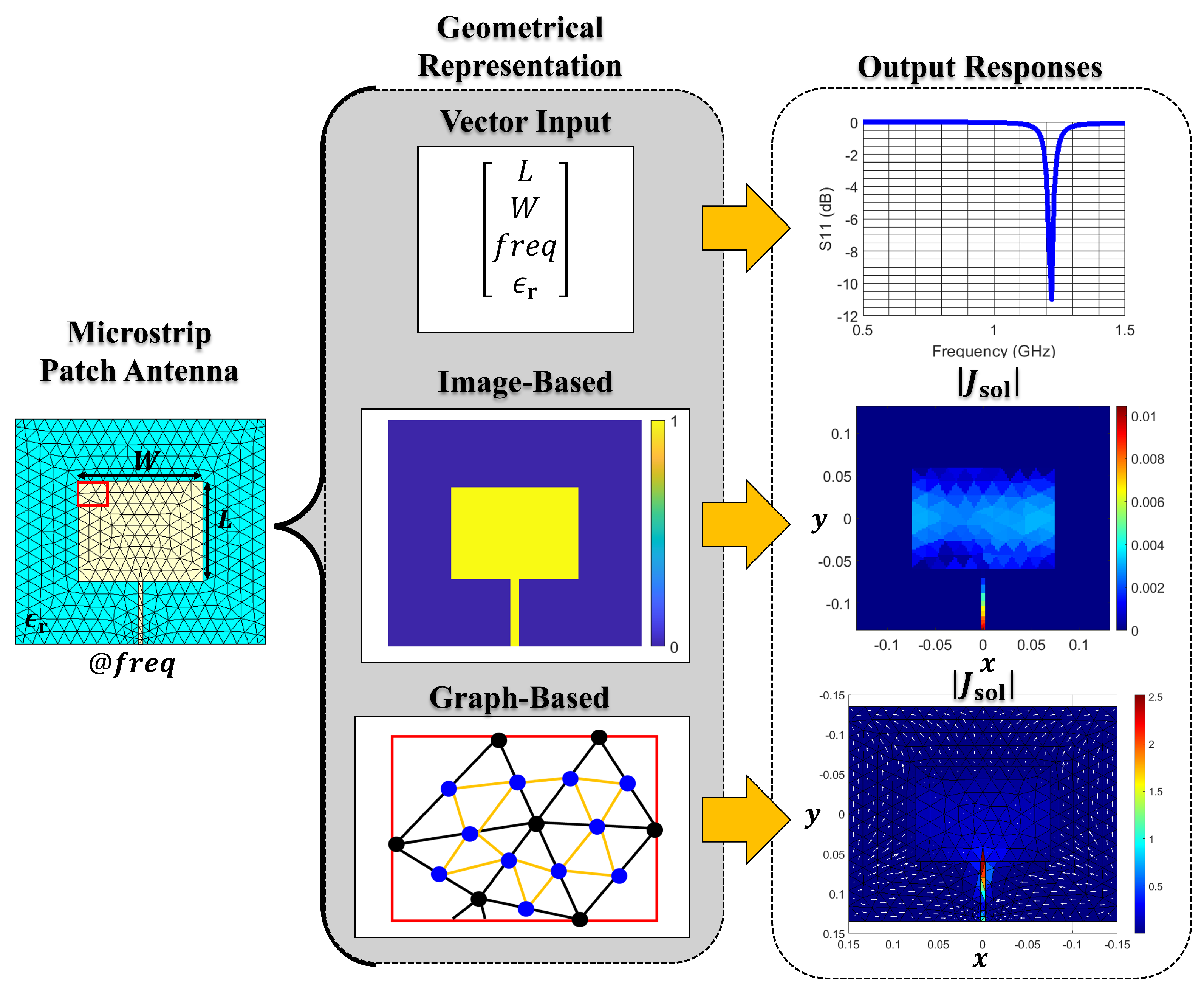
Moreover, selecting the appropriate ML approach is critical, and depends on the desired objective. Based on the literature, there are no specific ML model selection guidelines. However, one can narrow the selection based on how one would best represent the data of the specified task, as shown in Figure 2. For example, in [16], an N-element Yagi-Uda array at 165 MHz is considered, where the design variables include the length of all the antenna elements (i.e., the reflector, the driven element, and the $N-2$ directors), and the distance between each of them. In this scenario, the desired output specification is the directivity response in the forward direction ($\theta ={90}^{\circ }$, $\varphi =0^{\circ }$). Here, the input variables can be represented as a column vector of length $2N$, where the output is the single directivity value. In turn, one can utilize a variety of networks, like a dense forward-feeding neural network as in [16], a Kriging regression model [17], or a deep learning approach [8]. If multiple output specifications are considered, either multiple-output or several single-output regression models are suitable options [18]. Another modeling scenario is when the engineer requires the near-fields or current distributions along the antenna surface. For example, in [19], the electric near-field data of a microstrip patch antenna from 4 GHz to 6 GHz is considered. The near-field values are obtained along a 64 × 64 plane (with dimensions $1.5{\lambda }_{\mathrm{c}}\times 1.5{\lambda }_{\mathrm{c}}$, and ${\lambda }_{\mathrm{c}}$ is the wavelength at 5 GHz) positioned 1 mm above the microstrip patch. In this case, the design variables include the antenna geometry (length, width, and inset-gap feed), the substrate permittivity, and the frequency. Because the output is a $64\times 64$ sized matrix, DL image-based models (e.g., auto-encoders, generative models, etc.) are a suitable choice. In [19], a convolutional-based DL model was used, where the input parameters were also represented as $64\times 64$ images. Finally, other modeling scenarios include learning the mathematical operator, like the combined-field integral equation (CFIE) operator [20] of the forward problem. This approach would enable the same ML model to solve a variety of different structures without requiring re-training. The main challenge lies in representing arbitrarily shaped structures, which vary significantly, and cannot easily be captured using conventional input formats like column vectors or image-based methods. Additionally, the output solution should be adaptable and scalable in resolution to be able accurately represent structures with finer details, such as curved edges. A promising ML model solution to handle unstructured data is based on graph neural networks (GNNs) [21]. Here, arbitrarily shaped 3D metallic structures are modeled using triangles [based on Rao–Wilton–Glisson (RWG) [22] basis functions] and solved via the CFIE using MoM. GNNs learn on graph data, which is a collection of nodes connected by edges that represent relationships between the nodes. In this scenario, the RWG functions are considered nodes connected by edges to any adjacent RWG function, where the scalar current solution of the CFIE is learned.

After selecting the appropriate data representation and model topology, the ML modeling procedure continues via a design of experiments approach, where a design space is defined and a sampling plan is employed. Specifically, the lower and upper bounds of each design variable are specified, and a predetermined number of samples are generated to construct an initial surrogate model. These variable ranges are typically informed by the engineer’s expertise or relevant reference designs. The initial sampling plan aims to explore the design space, often utilizing random sampling or uniform sampling methods (e.g., Latin Hypercube Sampling (LHS)) [18]. The number of initial samples depends on the specific problem requirements and is constrained by the available computational resources. To enhance the model’s local accuracy (i.e., particularly in desirable design regions) additional samples are strategically allocated as needed. Regardless of the problem, the primary challenge is training the model to achieve a level of accuracy sufficient to replace the full-wave solver. Notably, this task typically depends on the number of samples available from the full-wave solver. However, obtaining a single full-wave evaluation can be very time-consuming. This problem is intensified as the number of input design variables (or output variables) increases since the required number of training samples increases exponentially with the number of design variables. This problem is known as the curse of dimensionality. In response, the EM scientific community has focused on deriving ML methods that require far fewer full-wave simulation samples to achieve comparable model accuracy.

One set of approaches focuses on limiting the modeled design space to specific regions of interest. Specifically, in antenna design, where the goal is to obtain high-performing designs. Initially introduced in [23], the constrained sampling technique uses optimal reference designs, from single objective optimization, to generate a polygonal-based design region. This work was advanced in [24] to include two design objectives in the constrained region definition. Finally, in [25], the approach was fully generalized based on triangular functions to define an arbitrarily shaped constrained design region based on reference designs containing any number of design objectives. Although it is highly efficient, this approach relies on the knowledge of optimal or near-optimal reference designs, limiting its application. Another way to reduce the simulation data required for training is to utilize multi-fidelity (MF) methods, which are also referred to as variable-fidelity methods [26]. The core concept assumes that the EM structure can be solved using different methods of varying accuracy. Specifically, these approaches assume the existence of a low-fidelity (LF) method, which is less accurate but significantly faster to solve. This computationally cheap model is used to train an initial coarse ML model to explore the design space (via an appropriate sampling plan) and roughly identify near-optimal regions. Then, the accuracy of this initial surrogate model is sequentially improved by acquiring additional data samples from these near-optimal regions. All these additional samples are obtained from the high-fidelity (HF) model, which is generally based on extensive full-wave simulations.

2.1. Multi-Fidelity Modeling

Unlike alternative approaches, multi-fidelity-based ML models can learn from two uneven sets of MF data [18]. Notably, these approaches assume that the LF model exhibits similar characteristics to the HF response. In turn, MF modeling takes advantage of this assumption to express the HF response, denoted as $y_{\mathrm{HF}}$, as some correction or transformation of the LF response, denoted as $y_{\mathrm{LF}}$, as:

$$\begin{array}{c}\hfill y_{\mathrm{HF}}=f_{\mathrm{w}}(·)y_{\mathrm{LF}}+f_{\mathrm{b}}(·),\end{array}$$

(1)

where $f_{\mathrm{w}}(·)$ and $f_{\mathrm{b}}(·)$ are the unknown correction functions to be found. In general, learning these correction functions results in more accurate models compared to learning the $y_{\mathrm{HF}}$ response directly from the input parameters. This section provides: (a) an overview of available MF surrogate models, (b) a detailed review of low-fidelity approaches, and (c) a discussion on current challenges and future research directions.

2.1.1. Co-Kriging Regression

Co-Kriging has been extensively used to derive MF models. Notably, co-Kriging is a probabilistic-based ML model based on the Kriging basis function, which uses the correlation Ψ between training data pairs to model the output response [18], as:

$$\begin{array}{c}\hfill \mathrm{\Psi }(x,x^{*})=ex{p}^{({\sum }_{\mathrm{n}=1}^N-{\theta }_{\mathrm{n}}|x_{\mathrm{n}}-x_{\mathrm{n}}^{*}{|}^{\rho })},\end{array}$$

(2)

where N is the number of samples, $\theta$ is the function width hyperparameter, and $\rho$ is the function’s “smoothness” hyperparameter. Notably, the Kriging method assumes that the underlying model function is smooth and continuous. For most antenna problems, $\rho$ is generally fixed at $\rho =2$ (also referred to as the Gaussian correlation function), and $\theta$ is determined by a meta-heuristic optimization of the function’s maximum-likelihood estimation (MLE) value, within the ranges of $\theta \in [{10}^{-2},{10}^3].$

Co-Kriging extends the Kriging method by correlating multiple uneven sets of varying fidelity. The most common approach follows the auto-regressive model of Kennedy and O’Hagan [27], which is based on the assumption (a Markov property) that the HF data are exact and that all errors lie entirely on the LF data. In turn, the HF response can be expressed as in (1), where the first correction function becomes a scalar, $f_{\mathrm{w}}(·)=\beta$, and the second correction function $f_{\mathrm{b}}(·)$ is modeled by a Gaussian process. Here, the Gaussian process is the residual between the input parameters of the available HF and LF samples, $x_{\mathrm{HF}}$ and $x_{\mathrm{LF}}$, respectively. In turn, most approaches utilizing co-Kriging will create an initial surrogate based on only LF data. Then, this model is explored to identify optimal regions in the design space. Specifically, to obtain a set of non-dominated designs for the m number of desirable specifications, i.e., a Pareto set of designs. Different Pareto designs are chosen and evaluated in the HF model to (i): train the co-Kriging model and (ii) calculate the modeling error. The resulting co-Kriging model is re-explored to fine-tune the optimal regions found. This iterative process is repeated until the model converges to a pre-defined tolerable error threshold.

2.1.2. Deep Learning MF Models

Significant technological advancements in artificial neural networks (ANNs) and deep learning (DL) have influenced many computational modeling approaches and solutions for electromagnetic systems. Consequently, these advancements have led to ANN-based MF approaches following the fundamental concepts of the co-Kriging method. Specifically, instead of using the Kriging method, these approaches utilize ANNs to calculate the correlation between the low-fidelity and high-fidelity data sets [28]. Notably, starting from (1), ANNs (or DL-ANNs) can be used to model the multiplicative correlation function $f_{\mathrm{m}}(·)$, and additive correlation function $f_{\mathrm{a}}(·)$. Unlike its co-Kriging counterpart, these ANN-based models can exploit non-linear activation functions (e.g., $tanh$ function) to capture non-linear correlations between the low- and high-fidelity models. However, this comes at the cost of increasing the model construction difficulty, such as selecting appropriate neural network hyperparameters (e.g., number of hidden layers, number of neurons, etc.), model optimizers (e.g., ADAM), and training loss functions (e.g., mean squared error). Depending on the chosen neural network topology, the training can become quite time-consuming, limiting its application as compared to co-Kriging approaches.

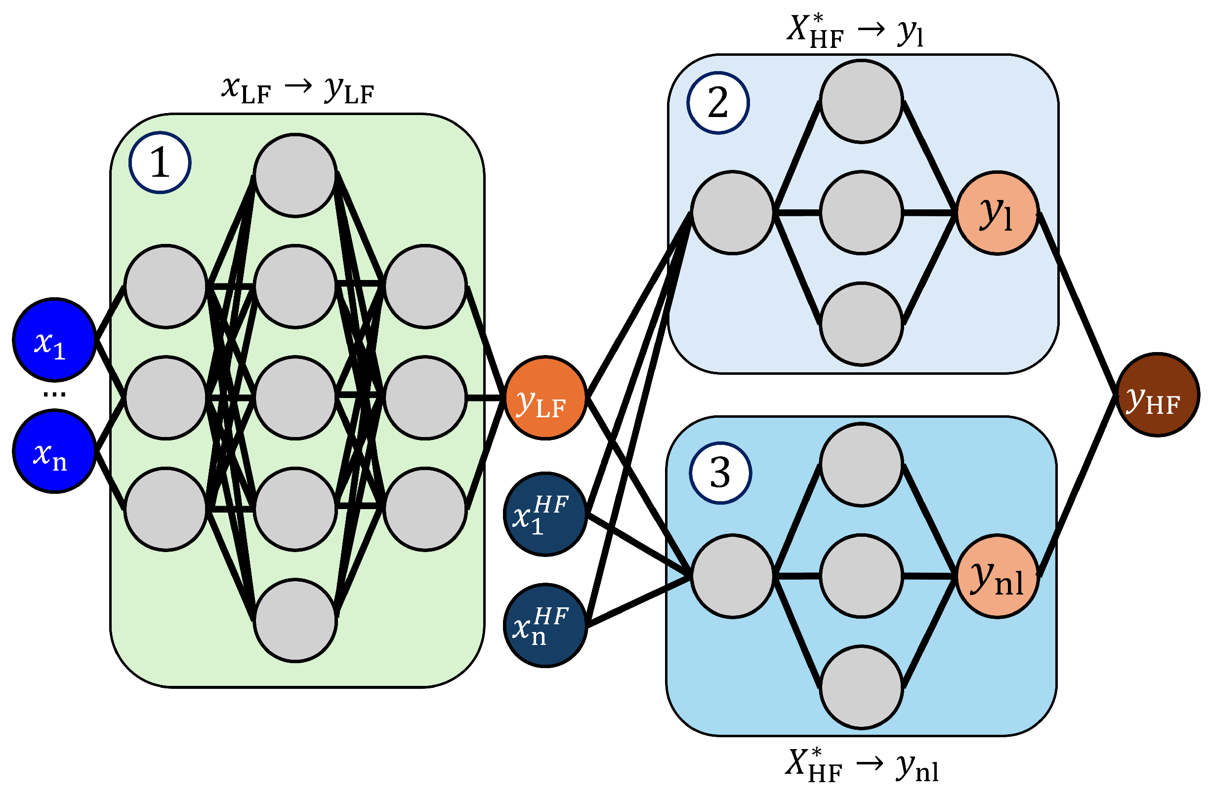
As we discussed previously, designing the neural network topology is challenging. This challenge is exemplified in the selection of an appropriate correlation function model. In regards to the forward problem, these ANN-based MF models have not been studied extensively. The ANN-based MF model from [28] was adapted in [29] to train an MF model to optimize different antenna structures. Here, as shown in Figure 3, the model is a stacked network topology, consisting of three individual fully connected forward-feeding networks (FCFFNs). This approach models the high-fidelity response, $y_{\mathrm{HF}}$ as a combination of the linear and non-linear correlation between the LF and HF responses, as, $y_{\mathrm{HF}}=y_{\mathrm{l}}+y_{\mathrm{nl}}$. In turn, the first model maps the LF input parameters $x_{\mathrm{LF}}$ to the low-fidelity responses $y_{\mathrm{LF}}$. The low-fidelity model output is appended to the HF input parameters $x_{\mathrm{HF}}$, as $[y_{\mathrm{LF}},x_{\mathrm{HF}}]$, denoted as $X_{\mathrm{HF}}^{*}$, and used as the input to the remaining two models. The last two models learn the output $y_{\mathrm{l}}$ and $y_{\mathrm{nl}}$ based on the $X_{\mathrm{HF}}^{*}$ responses, where the two outputs are combined to calculate $y_{\mathrm{HF}}$.

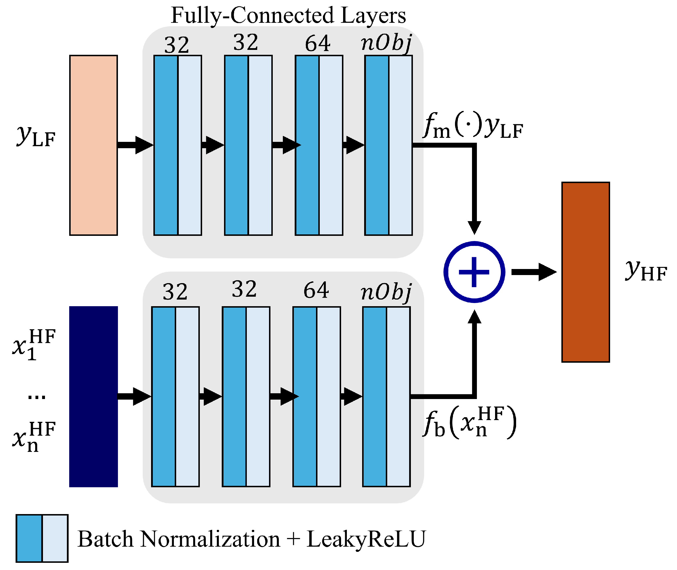
A similar deep learning MF approach was proposed in [30], as shown in Figure 4. The LF response is the input to a FCFFN, while the geometrical parameters are the input to a second FCFFN. The outputs of these models are the $f_{\mathrm{m}}(·)y_{\mathrm{LF}}$ and $f_{\mathrm{b}}(·)$ terms, respectively. In this scenario, both networks utilize LeakyReLU activation functions to capture the non-linear correlations. Then, the two outputs are summed to obtain the HF response as in (1). To the authors’ best knowledge, refs. [29,30] are the only ANN-based MF models investigated for EM forward modeling. However, there are many research works on ANN-based MF models in other scientific fields, like acoustics [31], manufacturing [32], and material science [33], to name a few. As such, these ANN-based approaches have high potential in the EM domain, which can be a future research direction.

2.2. Low-Fidelity Models

In summary, once the appropriate MF model is selected, the main challenge in training the model is in obtaining the LF model information. This challenge is based on two key assumptions: (a) that LF information is available within the modeling process, and (b) that the LF model shares the same underlying characteristics as the HF model. In this section, we will review different approaches used to generate LF models.

2.2.1. Coarse-Mesh Models

The most readily available LF modeling approach involves solving full-wave simulations utilizing a significantly coarser representation (e.g., lower mesh density) of the studied EM structure. Consequently, the simulations are accelerated at the expense of accuracy. This approach has seen the most extensive use in MF modeling, as most commercially-available software offer features that allow for simulation adjustments. However, as discussed in [34], the main challenge in implementing this approach is in appropriately reducing the model resolution to (a) sufficiently model the underlying physics of the model, and (b) provide adequate computational efficiency. For example, as shown in Figure 5, the LF model for a loop antenna can be obtained empirically by analyzing the changes in the broadside directivity responses as the model resolution is reduced. Here, the model resolution is measured by the number of discretization elements $N_{\mathrm{dis}}$. Notably, as the $N_{\mathrm{dis}}$ value decreases, the error in the response increases, until at around $N_{\mathrm{dis}}<150$, where the LF model starts to fail to capture the physics of the problem.

Table 1. Solution time of a broadband monopole antenna with varying simulation model densities.

${\mathit{N}}_{\mathbf{dis}}$	Time (s)	Acceleration 1
130	22	3.0
150	23	2.9
160	27	2.5
209	28	2.4
370	64	1.0
450	67	1.0

¹ When compared to $N_{\mathrm{dis}}$ = 450.

shows the solution time associated with the $N_{\mathrm{dis}}$ value, along with the acceleration rate when compared to the highest discretization value. In this scenario, the $N_{\mathrm{dis}}=160$ is a promising LF model selection, which can provide an average time improvement of about $2.4$ times.

2.2.2. Equivalent Circuit Models

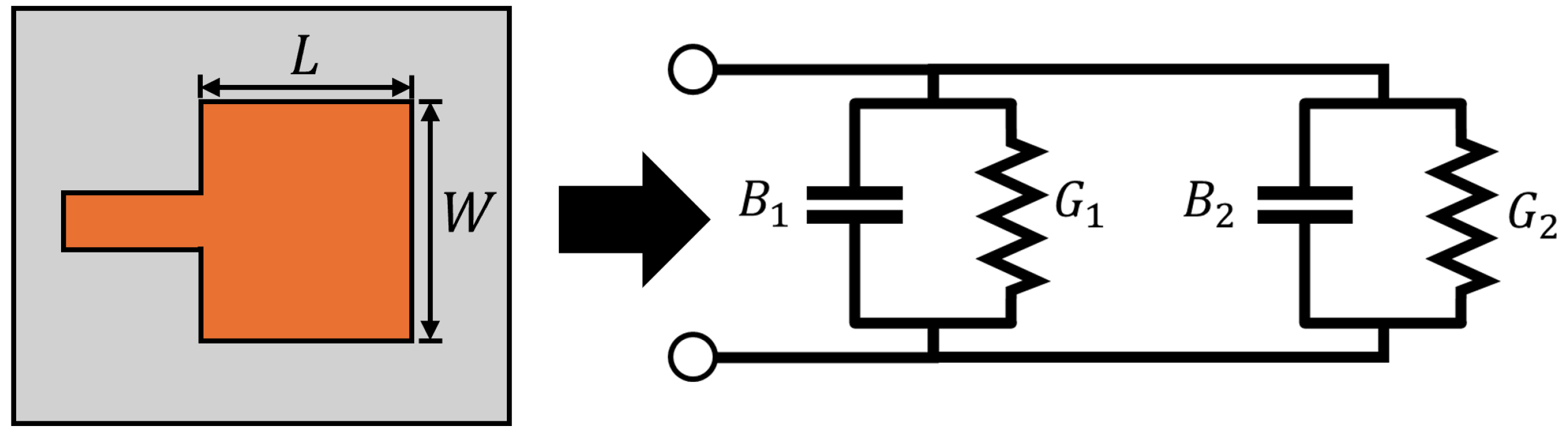
An alternative LF modeling approach is based on constructing equivalent circuit models to approach the desired antenna response [17]. Specifically, using commercially available software, like Keysight’s ADS, or fundamental antenna theory [35], to model an antenna design. For example, as shown in Figure 6, the two radiating slots of a rectangular microstrip patch antenna (for the dominant modes) can be modeled by an equivalent admittance

$$Y=G+jB,$$

(3)

where G is the conductance and B is the susceptance, separated by a transmission line with low impedance $Z_{\mathrm{l}}$ of length $l_{\mathrm{tl}}$. Here, the LF modeling procedure calculates G and B based on the substrate material, length, width, and operating frequency of the patch, where the height of the patch is assumed to be less than a tenth of the wavelength. In turn, this equivalent model can be used to obtain the input impedance $Z_{\mathrm{in}}$ of the microstrip patch, which can be used in impedance matching, or to calculate the return loss in a closed-form fashion. In the reviewed work, there is no reported LF solution time. Instead, the number of high-fidelity samples used to obtain the final MF model was reported. Notably, the final MF model achieves sufficient accuracy using less HF samples. Although this method offers a well-structured solution for obtaining an LF model, it lacks practicability and can suffer from high inaccuracies.

2.2.3. Numerical Eigenfunction Expansions

Another LF modeling approach is based on analytical models of the studied EM structure. This method was first introduced in [36], where eigenfunction expansion (EE) information is exploited to generate an approximation of the HF response. Here, the eigenfunction expansions for well-known EM structures (or canonical structures), like the loop and horn antenna, are known a priori. For non-canonical or arbitrary structures, the eigenfunction expansions need to be derived by solving a boundary-value problem based on [37]. The basis of this approach follows three key points, (1) the canonical domain is completely defined by a set of eigenfunction expansions, (2) the canonical domain completely encloses the arbitrary domain, and (3) any arbitrary structure can be represented as an alteration or perturbation of a canonical domain.

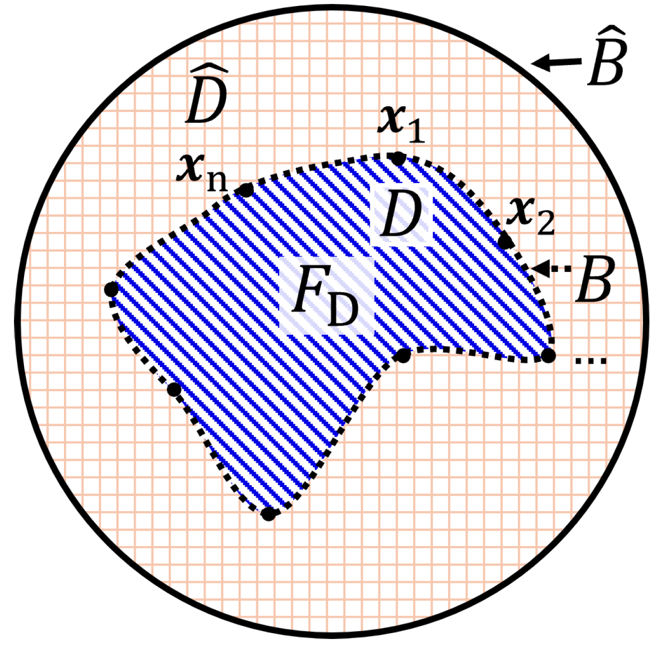
As shown in Figure 7, the canonical domain and the arbitrary domain are denoted as $\widehat{D}$ and D, respectively. They are defined by boundaries denoted as $\widehat{B}$ and B, respectively. First, following point (1), the field inside $\widehat{D}$ is completely known. Then, following point (2), because domain D is completely inside $\widehat{D}$, the field values along boundary B are also known. Finally, following point (3), the field inside D can be expressed as a perturbation of the fields in $\widehat{D}$, as:

$${\mathbf{F}}_D=\sum _{\mathrm{m}=1}^{\infty }{a}_{\mathrm{m}}{\widehat{\mathbf{F}}}_D\left({\mathbf{x}}_{\mathrm{n}}\right),$$

(4)

where $a_{\mathrm{m}}$ are the unknown perturbation coefficients to obtain after truncating the summation to M significant modes and enforcing the appropriate boundary conditions, ${\mathrm{\Psi }}_{\mathrm{bc}}$, along B. In [36], these boundary conditions were based on the expected field behavior at the known location of perfectly electrical conductors (PEC) and perfectly magnetic conductors (PMC). In [36], this approach was used to approximate the electric far-fields of arbitrarily-shaped patch antennas, where the LF model could provide sufficiently accurate responses in 4 s, compared to the HF model that solved in 3 min. In this scenario, the LF model is about 45 times faster than the HF model. Here, the authors did not compare the MF model to a traditional ML model (built only using HF samples), instead they compared to a model using an LF model built on the coarse-mesh method. Notably, the models trained based on EE were comparable in accuracy to the coarse-mesh method, where an average 2.8 times improvement across the entire modeling procedure was reported. Although this EE-based method is more practical than using equivalent circuit models, and in some cases significantly faster than the coarse-mesh approach, the EE-based approach cannot handle highly complex problems with very fine features.

2.2.4. ML-Based Techniques

Lastly, an innovative approach to obtaining an LF model involves leveraging a pre-trained model with lower accuracy, either in an adjacent design region of the same problem or for a closely related problem. This approach is rooted in the concept of transfer learning: when the underlying problem undergoes minor changes, the modeled wave behavior remains largely consistent [38]. Importantly, the LF model does not need to achieve high accuracy, as its primary goal is to capture the intrinsic characteristics of the HF model. The pre-trained model can then be employed to generate data for an MF modeling approach. A key limitation of this technique is that the input design space (i.e., the number of variables) and the output response must remain the same. This idea is applied in [30], where the out-of-distribution (OOD) generalization property of a DNN is exploited to make suitable approximations outside of the original design region. This enables the rapid generation of approximate LF data, which is subsequently used to train a model for the new region. This concept, similar to knowledge transfer, continues to gain traction in ML and computational sciences [39,40]. Its potential to enhance efficiency and flexibility in modeling complex systems makes it a promising area of ongoing research and development.

2.3. Discussion

Based on the available literature, training an ML model based on MF data generally reduces the number of HF samples required to achieve sufficient accuracy. This assumes that the LF data shares the same underlying characteristic as the HF data, allowing the model to learn on a correction function rather than the complete physics of the problem. As a result, the computational cost of training the MF model is significantly reduced.

Table 2. Summary of multi-fidelity forward problem approaches in the literature.

Ref.	Problem-Type	ML Type	LF Model	Number of Variables	Samples Used	Error	Advantage
[17]	Wideband Bandstop Microstrip	Adaptive response correction optimization based on third-order polynomial or cubic spline functions.	Equivalent-Circuit Model via ADS	5	4	N/A	On average, reduces the HF evaluations needed to correct the LF response by nearly 51%.
	Capacitively Coupled Dual-behavior Resonant Filter			4	$[5,4]$ *	N/A
	Low-pass Elliptical Filter			6	3	N/A
[26]	Dualband Dipole	Trust-region-based optimization scheme utilizing variable-resolution models.	Coarse-Mesh Model via CST	6	63.3 †	N/A	Reduces computational cost by 40%.
	Triple-band Dipole			10	127 †	N/A	Reduces computational cost by $30\%$.
	Low-pass Elliptical Filter			10	51.1 †	N/A	Reduces computational cost from $30\%$ to $60\%$.
[29]	CPW-fed Monopole Antenna	Multiple stacked fully connected forward-feeding neural networks using L hidden layers.	Coarse-Mesh Model via CST	4	20	NMSE $=2.4\%$	Achieves $\le 5\%$ error using only $10\%$ available HF samples.
	Dual-frequency Dual-sense Circularly Polarized Slot Antenna			8	490	NMSE $=\le 4.0\%$	Achieves $\le 5\%$ error using only $70\%$ available HF samples.

* For polynomial and cubic splice functions, respectively. ^† Total computational cost in terms of HF sample evaluations. NMSE: Normalized Mean Squared Error.

and

Table 3. Continuation of summaries of multi-fidelity forward problem approaches in the literature.

Ref.	Problem-Type	ML Type	LF Model	Number of Variables	Samples Used	Error	Advantage
[30]	Two-layer Bandpass Complementary Metasurface	Two stacked fully connected forward-feeding neural networks using L hidden layers.	Extrapolation property of pre-trained surrogate model	5	2500	MSE $=2.5\times {10}^{-3}$	Overall reduces computational cost by $30\%$.
	Three-layer Dualband Metasurface			6	1736	MSE $=12.6\times {10}^{-3}$	An ML-model based on only HF data requires 2480 samples to achieve an MSE $=12.4\times {10}^{-3}$.
[36]	N-element Uniform Loop Antenna Array	Multi-objective surrogate-based optimization using co-Kriging model.	Eigenfunction Expansions	5	54	MRE $=2.87\%$	Accelerates entire MF optimization process by $2.8$ times. **
	Pyramidal Horn Antenna			4	24	$7.20\%$	Accelerates entire MF optimization process by $2.2$ times. **
	Star-shaped Probe-fed Microstrip Patch Antenna			3	15	$2.78\%$	Accelerates entire MF optimization process by $2.6$ times. **

** Compared to the coarse-mesh based MF model. MSE: Mean Squared Error. MRE: Mean Relative Error.

highlight key aspects of recent MF approaches related to the forward problem. Notably, MF modeling schemes can achieve computational cost reductions ranging from $30\%$ to $90\%$ compared to traditional single-fidelity approaches. These savings can be further enhanced by selecting an LF model that provides the highest efficiency and the most correlated responses with the HF model. As discussed in [26,36], choosing an LF model with slightly less correlation (or greater inaccuracy) can increase the HF samples needed to achieve the desired accuracy. Nevertheless, this approach remains more efficient than traditional single-fidelity surrogate models.

As shown in Figure 5, selecting the fastest response will most likely lead to a need for more HF samples to correct the LF responses, potentially reducing the overall computational savings. However, the selection of the optimal LF model is highly problem-specific. The coarse-mesh method is the most universally applicable approach to implement, as it is based on coarsening an already existing HF model. Conversely, using approaches like the equivalent circuit approach or EE-based methods can significantly reduce computational costs but may be less effective if the problem’s complexity is too high. Because the number of HF samples required heavily depend on the specific task, there is no “fair” comparison that can be made to generalize the improvement from one LF model to the other. In general, the bottleneck of the computational cost saving is based on the HF model. For example, consider a scenario where 2 HF samples are required to correct an initial surrogate model built from 10 LF samples. If the HF model takes 5 min to evaluate and the LF model takes 1 s, the total time for MF modeling will be about 10 min. In comparison, a traditional surrogate model relying solely on HF samples would take approximately 50 min to train using 10 HF samples. In this case, the total training time is reduced by a factor of 5. For the sake of argument, if the LF model takes 10 s instead of 1 s, the total time will amount to nearly 12 min. Now, if the HF model takes 10 min to run, the two MF model examples would take about 20 min, and 22 min, respectively. Meanwhile, the traditional approach would need nearly 1 h and 40 min to train. Thus, as long as a sufficiently efficient and accurate LF model is chosen, significant time-saving can be achieved.

Another critical factor in the MF modeling process is the choice of the underlying correction method. In [17], an adaptive response correction approach reduced the number of required HF samples by nearly half compared to the standard space mapping method. Similarly, in [30], a DNN-based MF model achieved an MSE of $12.6\times {10}^{-3}$, significantly outperforming the co-Kriging model, which only achieved an MSE of $71.5\times {10}^{-3}$. This illustrates a major limitation of Gaussian-based models, which tend to struggle with high-dimensional spaces and large datasets [18]. To this, the literature indicates a lack of image-based or unstructured data-driven MF modeling approaches within the EM community. Most current methods tackle relatively low-dimensional problems (≤15 variables) and small datasets (sample size $\le 5000$). This direction stems from an emphasis on optimal design through simulation, usually constrained by factors like fabrication tolerances. Hence, surrogate-assisted approaches aim to improve model accuracy primarily in desirable regions of the design space to achieve globally optimal solutions. As a result, forward modeling procedures are commonly less concerned with overfitting and more concerned with converging to local non-optimal solutions. Moreover, unlike in other fields, EM simulation data is free from measurement noise and fabrication errors, which would be primary reasons for overfitting. However, in cases where general-purpose models are required, overfitting can be mitigated by using a sufficiently large sampling plan and implementing a proper training-test split. For neural networks, this includes restricting the number of training epochs to prevent overtraining.

In regards to current ML methods for antenna design and forward analysis, a key limitation is their focus on relatively simple geometries.

Table 4. Summary of ML-based forward problems in the literature.

Ref.	Problem-Type	ML-Type	Number of Variables	Samples Used	Error	Advantage
[7]	Inter-chip Wireless Antenna	Gaussian process-based surrogate approach.	10	300	N/A	$7\times$ faster compared to meta-heuristic method.
	4-element Linear E-patch Array		19	600	N/A	$3\times$ faster compared to meta-heuristic method.
	2D Patch Antenna Array		7	320	N/A	$3.5\times$ to $4.3\times$ faster compared to meta-heuristic method.
[8]	Miniaturized Rat-race Coupler with Meandered Transmission Lines	A two-stage modeling approach that utilizes a set of properly connected mini-neural network structures.	6	316	RRMS $=2.3\%$
	Miniaturized Branch-line Coupler with Compact Microwave Resonant Cells		10	326	RRMS $=2.3\%$	Achieves on average $3\%$ relative rms (RRMS) error using ≤350 HF evaluations.
	Equal Power Split Dualband Power Divider		7	278	RRMS $=3.5\%$
[9]	RHCP Microstrip Linear Antenna Array	Parallel use of two deep neural networks that utilize two complementary loss functions.	$[16,32,64]$	8000	N/A	Obtains solution in ≤0.12 s compared to traditional that solves within 2 h.
	CP Crossed-dipole Antenna		128	8000	N/A	Obtains solution in ≤0.24 s compared to traditional that solves in 6 h.
[16]	N-element Yagi Antenna	Traditional metaheuristic optimization assisted via a fully connected multilayer perceptron (FC-MLP) of L hidden layers.	11	50 *	N/A	Runs in $36.4$ s compared to $65.4$ s and $123.4$ s of PSO and GA, respectively.
	Coaxial Probe-fed Slotted Rectangular Patch		10	104 *	N/A	Obtains optimal design in 320 HF evaluations compared to traditional BSO that obtains it in 2080 HF evaluations.
[19]	Near-field of Microstrip Gap-fed Patch Antenna	A convolution neural network-based approach for the estimation of near field data.	$64\times 64\times 3$	$\mathrm{85,680}$	RMSE $=0.0205$	$200\times$ faster than full-wave simulations.

* Epochs in surrogate-assisted optimization. RRMS: Relative Root-Mean-Squared Error. RMSE: Relative Mean-Squared Error.

and

Table 5. Continuation of summaries of ML-based forward problems in the literature.

Ref.	Problem-Type	ML Type	Number of Variables	Samples Used	Error	Advantage
[21]	Arbitrary PEC Objects	A physics-informed deep learning approach with the utilization of graph neural networks.	Unstructured	$\mathrm{32,400}$	MSE ≤ 8 × 10−3	Nearly $10\times$ faster than full-wave simulations.
[41]	Single Layer FSS	An inverse topological design method based on a FC-MLP layers combined with Mixer layer techniques.	900	3000	MRE $=1.29\%$	To obtain comparable results, meta-heuristic methods require ≥3000 full-wave evaluations.
	Double Layer FSS		1800	2400	MRE $=1.15\%$	Meta-heuristic fails to obtain comparable design.
[42]	Triple Layer FSS	A spatial inverse design method based on a FC-MLP-Mixer model.	$200\times 200\times 5$	1400	MRE $=0.14\%$	Unlike traditional methods, capable of synthesizing the topological structures of FSS’s with expansive degrees of freedom.

MSE: Mean Squared Error. MRE: Mean Relative Error ($L_2$ Norm).

provide a comprehensive summary of existing ML-based approaches, the problems they address, and their performance metrics. Including MF approaches, most forward modeling studies fall into three primary categories: (1) microwave circuit components, (2) planar single-layer microstrip antennas, and (3) single-unit-cell analyses. However, there is a notable lack of case studies addressing highly complex structures, such as phased arrays, beamforming networks, multilayer electromagnetic designs, ultrawideband antenna arrays, matching networks, etc. A unique approach is the work by [21], which trained a model using unstructured data capable of representing arbitrary geometries. Their approach utilized canonical structures, such as spheroids and hexahedrons, to train the model, which was then extended (via transfer learning) to analyze more complex structures, including missile-head and airplane-like shapes, while the model successfully handled the missile-head cases, it struggled to capture sharp features in the aircraft examples. This emphasizes the need for further advancements in ML techniques to address more challenging and demanding electromagnetic problems.

3. Machine Learning for the Inverse Problem

The electromagnetic inverse problem follows the reversal of the forward problem operation. Instead of calculating the EM structure response y given the input design parameters x, as $x\to y$, the aim is to find the unknown input design parameters for a measured or desired EM structure response as $y\to x$. The inverse problem is very challenging as it is (a) non-unique, as multiple sets of input parameters can generate the same observed or desired output response, (b) under determined, as the number of unknown input parameters often exceeds the available measured or desirable response data, and (c) ill-conditioned, since minor discretization errors or measurement noise can lead to considerable inaccuracies in the solutions. The severity of these challenges changes slightly depending on the type of inverse problem tackled. However, in general, the inverse problem requires approaches that address these challenges to obtain accurate solutions.

Recently, machine learning approaches have been employed to solve the inverse problem due to their excellent predictive ability and computational efficiency. Notably, ML-based methods have been successfully applied to many applications, such as inverse design [43,44], biomedical imaging [45,46], underground terrain imaging [47], and electronic device diagnosis (e.g., faulty arrays [48], and printed-circuit boards [49]). Similar to the forward problem, most of these approaches follow supervised learning techniques, which include semi-supervised or guided learning techniques. As shown in Figure 8, the inverse solutions generally fall under three classes of approaches: (1) identify the optimal geometrical parameters for a given design based on the desired response, (2) identify the locations of sources of error of a studied structure, and (3) identify the location, shape, and electrical properties of an unknown structure(s) embedded inside a region of interest based on its scattered fields. As discussed in Section 2, the selection of the model is heavily dependent on the specific problem, which also depends on the representation of the input (x)-output (y) pairs.

In the first class of approaches, for example in [43], a multi-branch artificial neural network is employed to design a short dipole planar array based on the desired directivity response $D_1$. The model estimates four key physical parameters, which include the horizontal and vertical element distances, denoted as $d_{\mathrm{h}}$ and $d_{\mathrm{v}}$, respectively, and the number of elements along the horizontal and vertical directions, denoted as $n_{\mathrm{h}}$ and $n_{\mathrm{v}}$, respectively. In turn, the model input was a single-valued input $D_1$ mapped to a four-length vector $x={\left[d_{\mathrm{h}}{d}_{\mathrm{v}}{n}_{\mathrm{h}}{n}_{\mathrm{v}}\right]}^T.$ In this scenario, the array element is pre-determined and the objective is to find its proper placement and distribution. In some scenarios, like in the inverse design of metasurfaces (MSs) or frequency selective sheets (FSSs), it is desirable to generate an arbitrary structure with the desirable output response. For example, in [44], a generative-based approach (i.e., utilizing a variational autoencoder, VAE) approximates the unit cell structures of an MS based on latent variables, which are selected based on specified scattering parameters. To represent arbitrary multi-layer planar structures, $52\times 52$ sized images are used, where the desired response was a vector with the amplitude and phase of the transverse electric and transverse magnetic transmission coefficients. Similarly, in [42], a multi-layer perceptron model is employed to learn the direct mapping between the target scattering parameters and arbitrarily shaped single-layer FSS structures. The input consists of an N length vector with the N reflection coefficient values across the frequency sweep and the output is the $30\times 30$ binary image of the FSS unit-cell topology.

Notably, the inverse modeling approach is closely related to the forward modeling approach, as the training data are based on a single or set of pre-selected antenna designs with their respective responses. In turn, many inverse design approaches follow a combination of forward and inverse models. For example, in [44], the encoder model learns a mapping between the design and the latent variables, and the decoder learns the mapping between the latent variables and the design. A third model learns a mapping between the latent variables and the transmission coefficients. In turn, the inverse design approach involves performing a surrogate-assisted metaheuristic optimization to obtain the optimal latent variables, which the decoder uses to generate the optimized unit cell structure. Similarly, in [50], a generative-based inverse model estimates the metasurface unit cell design parameters based on the target response. Then, a forward model predicts the actual response of the generated structure. Consequently, the two models work together to ensure accurate unit-cell design predictions.

The second set of inverse approaches focuses on the diagnosis of malfunctioning electronic devices by using near-field and far-field measurements. Notably, the objective of the model is to identify the sources of error. To this, the ML model will learn a mapping between the measured field and the location of broken or faulty components. In this scenario, the data representation depends on the type of measurements conducted. For example, in [48], the near-field measurements of a dipole and loop antenna array are collected along a rectangular surface, which can be represented as an image. In turn, the model learns to map the near-field image to a latent vector, which is used to calculate the surface currents of the arrays. Then, the reconstructed currents are used to identify the faulty array elements. Following the same concept, ref. [49] represents the measurements of a substrate-integrated waveguide (SIW) along a rectangular scanning surface as an image. Similarly, the SIW structure is represented as an image, where a k-nearest neighbor model is employed to classify the sources of error based on the images. Specifically, whether the fault is due to the feed lines or the vias.

Lastly, the third set of approaches aims to solve general microwave imaging problems also referred to as the inverse scattering problem (ISP). In this context, the object parameters to be determined include its physical and electrical properties, leading to a nearly infinite range of possible solutions. This review will focus on the solutions to electromagnetic ISPs, which pose unique challenges compared to inverse design or electronic device diagnostics. Unlike the latter cases, where the possible solutions are restricted to a predefined structure or a subset of known structures, electromagnetic ISPs involve completely unknown target structures, significantly increasing the complexity of the problem. This review provides a comprehensive overview of electromagnetic ISPs, and specifically, of machine learning-based methods. Notably, a brief overview of traditional electromagnetic ISP approaches is given for reasons of completeness.

4. Inverse Scattering Problem

Electromagnetic ISP techniques have recently become a cost-effective method for characterizing targets, such as identifying their location, shape, and material composition (e.g., permittivity and conductivity). Notably, they have been effective in radio and microwave applications, such as in non-destructive through-wall imaging [51], medical imaging and diagnosis [45,46], and commercial remote sensing [52]. Specifically, these approaches enable either qualitative or quantitative reconstruction of target properties based on scattered field information from a region of interest (RoI). Qualitative reconstruction refers to identifying the target’s electrical properties (e.g., permittivity and conductivity profiles), while quantitative reconstruction refers to identifying the target’s spatial properties (e.g., size, velocity, etc.). For example, in stroke diagnosis, a qualitative approach can identify critical tissue compositions in the brain essential for assessing a patient’s condition [53]. In contrast, quantitative reconstruction can be used in underground pipe maintenance to detect damaged sections through the ground [54].

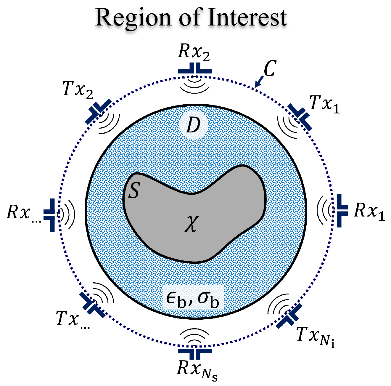
To illustrate the core concept of microwave inverse approaches, consider the scenario depicted in Figure 9. An object with an arbitrary shape, denoted as S, is located within an RoI, labeled as region D. This region is illuminated by electromagnetic waves from surrounding transmitters (Tx), and the scattered wave radiation is collected by a distributed array of receivers (Rx) along the contour C encircling D. In microwave imaging, this object is generally assumed to be a nonmagnetic, heterogeneous, and isotropic medium. It is characterized by its complex-valued relative permittivity,

$${ϵ}_{\mathrm{r}}={ϵ}_{\mathrm{Re}}\left(r\right)+1j{ϵ}_{\mathrm{Im}}\left(r\right),r\in D,$$

(5)

with a permeability set to ${\mu }_0=1$. For most microwave applications, the total scattered field $E_{\mathrm{s}}$ satisfies the inhomogeneous Helmholtz wave equation in the transverse magnetic (TM) configuration, where the total field can be expressed as,

$$E_{\mathrm{t}}\left(r\right)=E_{\mathrm{i}}\left(r\right)+k_{\mathrm{b}}^2{\int }_{D}G(r,r^{\prime })({ϵ}_{\mathrm{r}}\left(r\right)-1)E_{\mathrm{t}}\left(r^{\prime }\right)d{r}^{\prime },r\in D,$$

(6)

where $k_{\mathrm{b}}$ is the background medium wavenumber, $G(r,r^{\prime })$ are Green’s functions, and $E_{\mathrm{i}}\left(r\right)$ is the incident field. In turn, (6) is used to calculate the induced contrast current,

$$J=({ϵ}_{\mathrm{r}}\left(r\right)-1)E_{\mathrm{t}}\left(r\right),r\in D.$$

(7)

Then, the scattered field at the receivers can be expressed as,

$$E_{\mathrm{s}}\left(r\right)=k_{\mathrm{b}}^2{\int }_{D}G(r,r^{\prime })({ϵ}_{\mathrm{r}}\left(r\right)-1)E_{\mathrm{t}}\left(r^{\prime }\right)d{r}^{\prime },r\in C.$$

(8)

These governing Equations (6) and (8) are also known as the state and data equations, respectively. For convenience, these field-type equations can be re-written in compact form as,

$$E_{\mathrm{t}}\left(r\right)=E_{\mathrm{i}}\left(r\right)+G_{\mathrm{D}}{\displaystyle (}({ϵ}_{\mathrm{r}}\left(r\right)-1)E_{\mathrm{t}}{\displaystyle )},r\in D,$$

(9)

$$E_{\mathrm{s}}\left(r\right)=G_{\mathrm{C}}{\displaystyle (}({ϵ}_{\mathrm{r}}\left(r^{\prime }\right)-1)E_{\mathrm{t}}{\displaystyle )},r\in C,$$

(10)

where $G_{\mathrm{D}}$ is the numerical operator representing the evaluation of the second term in (6), and $G_{\mathrm{C}}$ is a numerical operator representing the evaluation of the integral in (8).

In the forward problem, (6) is solved to obtain the total field given the object. As discussed in Section 2, this is computationally expensive, especially when the object is more complex or D is electrically large. In the inverse problem, (6) is solved to obtain the dielectric contrast, $\chi \left(r\right)$, $r\in D$, of the arbitrary scatterer embedded within the background medium, using the measurements of the scattered field, $E_{\mathrm{s}}\left(r\right)$, $r\in C$. Notably, the dielectric contrast is expressed in terms of the complex-valued background medium permittivity, ${ϵ}_{\mathrm{b}}$ and conductivity, ${\sigma }_{\mathrm{b}}$, as,

$$\chi \left(r\right)=\left[{\displaystyle \frac{{ϵ}_{\mathrm{r}}\left(r\right)}{{ϵ}_{\mathrm{b}}-1}}-j{\displaystyle \frac{\sigma \left(r\right)-{\sigma }_{\mathrm{b}}}{{ϵ}_{\mathrm{b}}{ϵ}_0\omega }}\right],r\in D,$$

(11)

where $\omega =2\pi f$ and f is the solution frequency. In this scenario, the total field is also unknown, hence the inverse problem requires estimating both the total field and the dielectric contrast, leading to a highly nonlinear problem. Moreover, the scattering model’s non-linearities significantly increase when the object is electrically large or when multiple scatterers are involved. These factors, combined with the challenges discussed in Section 3, result in a highly complex reconstruction problem.

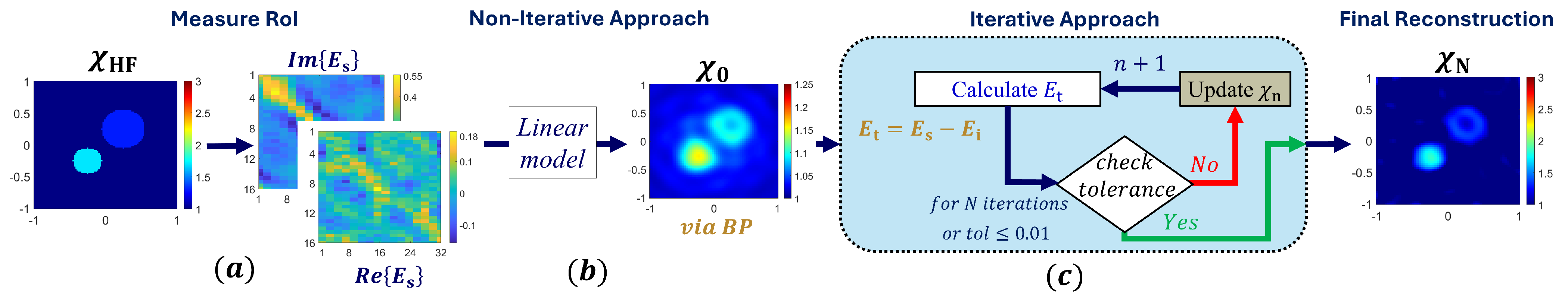
4.1. Non-Iterative Approaches

To achieve accurate inverse scattering solutions, it is essential to address the problem’s non-linearity, ill-posedness, and ill-conditioning. As shown in Figure 10, methods to alleviate these challenges include both non-iterative and iterative approaches coupled with regularization techniques. Non-iterative approaches often linearize the scattering model to approximate the solution, with the most popular approaches based on the Born and Rytov frameworks, also known as the first-order approximations [55]. These approximations are particularly effective under the “soft-scattering” assumption, which assumes that the object’s dielectric profile is roughly equal to that of the surrounding medium. In the Born approximation, the unknown field $E_{\mathrm{t}}$ in (6) is taken to be equal to the incident field $E_{\mathrm{i}}$, expressed as,

$$E_{\mathrm{s}}\left(r\right)\approx G_{\mathrm{C}}\left(\chi \left(r\right)E_{\mathrm{i}}\right).$$

(12)

Similarly, the Rytov approximation expresses the unknown field as a multiplication of the incident field and a phase correction parameter ${\mathrm{\Psi }}_{\mathrm{s}}\left(r\right)$, given as,

$$E_{\mathrm{t}}=E_{\mathrm{i}}{e}^{{\mathrm{\Psi }}_{\mathrm{s}}\left(r\right)}.$$

(13)

Notably, ${\mathrm{\Psi }}_{\mathrm{s}}\left(r\right)$ replaces the measured fields in the Rytov approach, which can be calculated as,

$${\mathrm{\Psi }}_{\mathrm{s}}\left(r\right)=ln\left[{\displaystyle \frac{E_{\mathrm{t}}\left(r\right)}{E_{\mathrm{i}}\left(r\right)}}\right].$$

(14)

In both scenarios, accurate reconstructions are obtained when the object’s contrast is sufficiently small, while the Born approximation excels at reconstructing electrically small objects and lower frequencies, the Rytov approximation obtains more accurate solutions for larger objects and in higher frequency scenarios. However, both will fail to reconstruct even slightly higher-valued contrast objects. Another popular non-iterative technique is back-propagation (BP), where the induced current of the hidden object is assumed to be proportional to the measured field, as [56],

$$J=\beta \left[G_{\mathrm{C}}^{*}\left(E_{\mathrm{s}}\left(r\right)\right)\right].$$

(15)

Here, $G_{\mathrm{C}}^{*}$ is the adjoint of the numerical operator $G_{\mathrm{C}}$. Then, the complex variable $\beta$ can be found by minimizing the quadratic error in the scattered field. Higher-order approximations have also been introduced to extend the first-order approximations to more practical scenarios, like, the extended BA and extended RA [57,58], but at the cost of increased algorithm complexity.

4.2. Iterative Approaches

To address the limitations of these approximate models, iterative techniques like the distorted Born iterative method (DBIM) have been developed [59]. These methods use first-order approximations as an initial guess, then iteratively refine them by minimizing a residual loss function, which is generally the difference between the measured field and the predicted field. Here, the predicted field represents the scattered field of the recovered object, which is obtained by solving the forward problem. However, this forward step substantially increases the computational cost of iterative approaches. Advanced iterative schemes improve efficiency by approximating the total field of the predicted contrast, thereby avoiding the need to solve the forward problem directly. In approaches like contrast source inversion (CSI), both the contrast and the total field are cast as optimization variables iteratively tuned by minimizing the residual function of the reconstruction [60], as,

$$Min:F(J,\chi )={\displaystyle \frac{\left|\right|E_{\mathrm{s}}-G_{\mathrm{C}}\left(J\right){\left|\right|}^2}{\left|\right|E_{\mathrm{s}}{\left|\right|}^2}}+{\displaystyle \frac{\left|\right|\chi E_{\mathrm{i}}+\chi G_{\mathrm{D}}\left(J\right)-J{\left|\right|}^2}{\left|\right|\chi E_{\mathrm{i}}{\left|\right|}^2}},$$

(16)

which measure mismatches between the source and data equations. This process uses Polak–Ribiere update steps to alternately refine the contrast and field at each iteration, eliminating the requirement to solve the forward problem. However, a successful reconstruction based on CSI heavily relies on the initial guess. To mitigate this problem, approaches such as subspace-based optimization methods (SOMs) were introduced. In SOMs, the currents associated with the total field are decomposed into deterministic (dominant) and ambiguous parts through the singular-value decomposition of Green’s operator [61]. The deterministic component can be uniquely determined for any incident field, while the ambiguous component is represented as a Fourier series with unknown coefficients to be solved. Thus, instead of updating the entire current at each step, only these unknown coefficients are adjusted, reducing the number of unknowns and alleviating the ill-conditioned problem. However, due to their iterative nature, these approaches remain unsuitable for real-time applications and may still fail if the initial guess is inadequate.

4.3. Machine Learning Approaches

To facilitate the complex reconstruction process for real-time solutions, machine learning techniques have been introduced to substitute or accelerate the iterative procedure. These include purely data-driven, or “data-to-image”, approaches that learn the direct mapping from measured fields to dielectric contrasts, $\chi =f\left(E_{\mathrm{s}}\right)$. By employing image-to-image deep learning, the measured fields are represented as a complex-valued image, which is then mapped to an image of the hidden object. However, a significant challenge for these data-to-image models is that they must learn the highly nonlinear and ill-posed relationship between the hidden object and the field, requiring large datasets for effective training.

A key distinction between the forward and inverse machine learning schemes lies in their definition of high-fidelity training data. In the forward approach, this refers to the ground truth response via full-wave simulations of a given structure. In the inverse approach, this refers to the ground truth dielectric contrasts of a given measured response. Notably, in real-world applications, the latter information may not be available. Additionally, unlike the design-of-experiments approach employed in the forward problem, data generation in the inverse problem is less exploitative, focusing instead on enhancing the model’s generalization ability (i.e., its accuracy across the entire region and beyond). Therefore, in inverse problems, it is common practice to utilize all the available HF data after the train–test split. In addition, the model must be trained on a diverse set of scattering geometries with arbitrary shapes and electrical properties. To define these arbitrary structures, the ISP community often uses well-known datasets, such as the MNIST and EMNIST datasets [62]. Another common approach involves randomly placing single or multiple canonical geometries (e.g., cubes, cylinders, triangles, etc.) within the RoI, potentially allowing them to overlap. Each scatterer is then assigned random permittivity and conductivity values. Once these structures are defined, the forward problem is solved to obtain the arbitrary structure’s scattered field using (9) and (10). Three examples of these training structure selection schemes are illustrated in Figure 11. This data generation process is computationally expensive as solving these equations for each sample has an associated computational complexity of $O\left(Mlo{g}_{2}M\right)$, where M is the number of discretization elements. It is important to note that these training structures are regularly employed in the general ISP problem. However, for focused applications, like biomedical imaging, these training structures may not be appropriate. Instead, a proper training dataset should be selected for the desired task, increasing significantly the difficulty of microwave imaging based on ML models.

Nonetheless, once trained, these data-to-image models can outperform traditional iterative methods in terms of accuracy and time. For example, in [63], a data-to-image model, based on the U-Net convolutional neural network, was trained using 475 samples of multiple circular cylinders with ${ϵ}_{\mathrm{r}}=(1,1.5]$. The model achieved reconstructions within 1 s, while maintaining a relative error of ≤14% for simple structures similar to the training data. However, for more complex examples outside of the training data, the model failed to produce meaningful reconstructions. This highlights the importance of (i) obtaining sufficient training samples, and (ii) carefully curating the example geometries within the training data, as these models may fail to generalize and reconstruct objects with highly irregular features (e.g., sharp edges) or higher permittivities.

To address this issue, more advanced data-to-image deep neural network architectures have been proposed [64,65,66].

Table 6. Summary of data-to-image approaches in the literature.

Ref.	ML Type	Input *	Output †	Training Data	Samples Used	Error	Comments
[63]	U-Net convolutional neural network.	$16\times 32$	$64\times 64$	Random Overlapping Cylinders (${ϵ}_{\mathrm{r}}=(1,1.5]$)	475	RE = $5.8\%$	Obtains reconstructions ≤1 s. Fails to generalize well.
[64]	Two-output-branch neural network based on U-Net and auto encoder.	$32\times 32$	$128\times 128$	EMNIST (${ϵ}_{\mathrm{r}}=[2,3]$)	5000	MSE = $9.2\times {10}^{-2}$	Achieves MSE $\le 6.0\times {10}^{-1}$ for out-of-training samples for anomaly detection. Evaluation time is not reported.
[65]	Deep convolutional generative adversarial network.	$20\times 20$	$20\times 20$	MNIST (${ϵ}_{\mathrm{r}}=(1,8]$)	5000	NMSE = $0.2$	Produces reconstructions within $0.03$ s compared to an iterative scheme that solves in 6 s, while maintaining an SSIM $=0.9$ for test samples. Achieves NMSE = $0.2$ and SSIM $=0.74$ for generalization examples.
[66]	Two-step deep learning model based on convolutional encoder–decoder and residual neural network.	$24\times 1$	$24\times 24$	MNIST (${ϵ}_{\mathrm{r}}=(1,8]$)	5000	NMSE = $0.1$	Produces reconstructions within $0.02$ s and achieves an SSIM $=0.9$ for test samples.
[67]	Deep generative model based on a low-dimensional manifold and Bayesian framework.	$12\times 12$	$64\times 64$	Random Overlapping Ellipses (${ϵ}_{\mathrm{r}}=(1,4]$)	$\mathrm{60,000}$	N/A	Achieves an SSIM = $0.85$ compared to an SSIM $=0.82$ of the BP-based solution in [63], where the DBIM method fails. Requires an iterative scheme making it unfavorable for real-time imaging.
[68]	Fully Connected Neural Network with L hidden layers.	$10\times 9$	$1\times 5024$	Custom Virtual Neck Phantoms	$\mathrm{30,000}$	NRMSE ≤ 0.35	Model with $L=5$ and 448 neurons can successfully capture tissue anomalies.

* Complex Valued Scattered Fields ($N_{\mathrm{i}}\times N_{\mathrm{s}}$). ^† Contrast Images. RE: Relative Error. MSE: Mean Squared Error. NMSE: Normalized Mean Squared Error. SSIM: Structure Similarity Index. NRMSE: Normalized Root Mean Squared Error.

summarizes the most recent approaches studied in this review. For instance, a deep two-output-branch neural network combining a U-Net and autoencoder (AE) has successfully reconstructed arbitrarily shaped scatterers within ${ϵ}_{\mathrm{r}}=3$ using 5000 training samples. In [65], a conditional deep convolutional generative adversarial network (cGAN) is developed to accurately reconstruct objects of arbitrary shape with ${ϵ}_{\mathrm{r}}=(1,8]$, employing 5000 training samples. Additionally, in [67], a deep injective generative model learned a low-dimensional manifold representation to reconstruct contrasts within ${ϵ}_{\mathrm{r}}=(1,8]$, utilizing $\mathrm{60,000}$ training samples. Despite these advancements, data-to-image approaches still demand a considerable number of training samples and prolonged training times. Notably, further investigation on the computational cost of these models is needed, as none of the referenced works reported their model training times.

4.3.1. Physics-Based Learning

Alternatively, the most promising machine learning approaches focus on providing solutions that either (a) accelerate the costly forward solution step, (b) replace and improve the iterative approach, or (c) correct a coarse reconstruction arriving from a first-order approximation or iterative scheme. The first category was discussed in Section 2, where an appropriate model is trained to provide fast solutions to the forward problem. The second and third categories are inverse-based tasks, where the main idea is that the model does not have to learn the direct mapping between the measured field and the hidden object, and instead focuses on performing a specific reconstruction sub-task. Notably, these approaches merge purely data-driven and physics-based techniques to leverage a priori information (i.e., low-fidelity data) and reduce the complexity of the problem. In addition, unlike in traditional supervised learning, the model loss function is not limited to predicting labeled data, but may also incorporate the minimization of the reconstruction residual loss functions. Due to the literature’s vague nomenclature, these approaches are not referred to as multi-fidelity models, although they do utilize datasets of variable fidelity to train their models. Notably, to maintain consistent with the studied literature, these MF models are referred to as physics-based models. As observed in the forward problem, these physics-based approaches generate more accurate models. However, unlike in the forward problem, the scientific community has not studied their effect on the amount of required training data. The following section reviews the two types of machine learning inverse tasks.

Iterative Replacement Models

The first set of physics-based approaches aims to replace the lengthy iterative correction process. Here, the model’s objective is to emulate a desired iterative process (e.g., BIM, etc), and learn to suitably update the predicted contrast and the total field (or contrast current source). In this scenario, because the trained model does not strictly follow the guiding update rules, it is capable of overcoming convergence issues and recovering objects where the traditional iterative scheme fails. This reconstruction is performed rapidly by the model allowing this to be used in real-time. Table 7 summarizes relevant approaches proposed recently in the literature. For example, in [69], an unrolling network is trained based on SOM, which is referred to as SOM-Net. The overall modeling process is summarized in Figure 12. At each step, the model outputs an induced current correction based on the previous induced current and the contrast approximation obtained analytically through SOM. In turn, the model loss function is based on supervised learning, such as predicting the induced current and the target permittivity, and guided learning, such as reducing the residual loss between the measured field and the predicted total field. Here, the model is trained with 5000 samples and demonstrated excellent generalization ability. On average, the model’s reconstructions achieved a $0.03$ lower root mean squared error (RMSE) and a $9\%$ improvement in the structure similarity index measure (SSIM) compared to SOM. Even in cases where the model did not show a distinct accuracy advantage, it significantly reduced the overall reconstruction time by $92\%$. A similar unrolling network approach was proposed in [70], where a residual network learns based on the CSI iterative scheme. Notably, this work utilized 2000 samples, achieving an average relative error of $1.4\%$ and an SSIM of $74\%$. The traditional CSI method’s performance was not fully reported, as it often failed to yield real solutions. In this scenario, the model reduced the total reconstruction time by $90\%$ compared to the CSI approach. In [71], a residual network is interpreted as a fixed-point iterative technique and utilized to learn the update steps based on the traditional BIM. Here, one model was trained using the supervised loss function, meanwhile the other was trained on the guided learning functions. Notably, both models were trained using $\mathrm{20,000}$ samples. The supervised model achieved a mean absolute error (MAE) of nearly $0.03$, while the guided model achieved an MAE of $0.12$. Despite these differences, both models significantly improved the reconstruction accuracy compared to the traditional BIM, which had a higher MAE of $0.2$. Additionally, both models drastically reduced the overall reconstruction times, achieving nearly a $99\%$ time reduction.

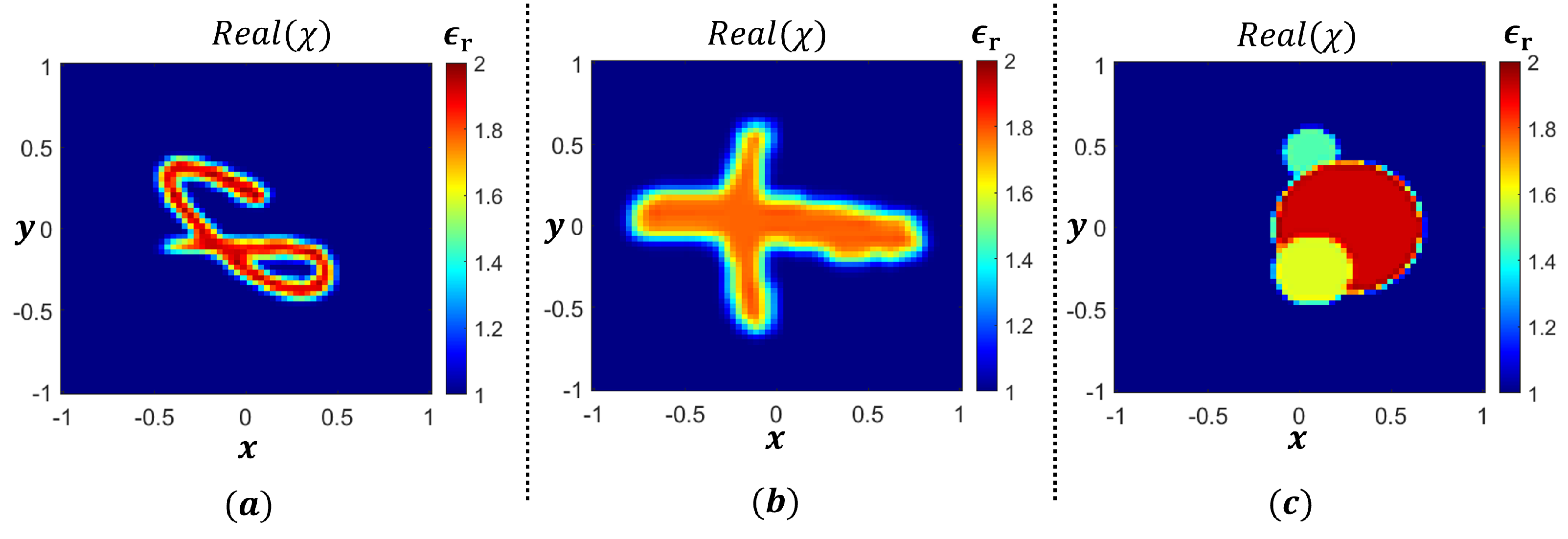
Figure 12. Illustration of the SOM-Net used in [69]. The model input includes an image of the deterministic induced current (for $N_{\mathrm{i}}$ illuminations) and the raw contrast image derived from BP. The model output is the final corrected induced current (two channels for real and imaginary components), which is used to obtain the predicted scattered field $E_{\mathrm{s}}$ and the final contrast reconstruction ${\chi }_{\mathrm{N}}$ following the SOM. The model topology follows a traditional U-Net layout [72], where the encoding steps follows a $2\times 2$ max-pooling layer followed by two $3\times 3$ convolutional layers with batch normalization and ReLU activation functions. The decoder operation mirrors the encoding step, where a $2\times 2$ up-convolution layer replaces the max-pooling step.

Figure 12. Illustration of the SOM-Net used in [69]. The model input includes an image of the deterministic induced current (for $N_{\mathrm{i}}$ illuminations) and the raw contrast image derived from BP. The model output is the final corrected induced current (two channels for real and imaginary components), which is used to obtain the predicted scattered field $E_{\mathrm{s}}$ and the final contrast reconstruction ${\chi }_{\mathrm{N}}$ following the SOM. The model topology follows a traditional U-Net layout [72], where the encoding steps follows a $2\times 2$ max-pooling layer followed by two $3\times 3$ convolutional layers with batch normalization and ReLU activation functions. The decoder operation mirrors the encoding step, where a $2\times 2$ up-convolution layer replaces the max-pooling step.

Table 7. Summary of iterative replacement approaches in the literature.

Ref.	ML Type	Input *	Output †	Training Data	Samples Used	Error	Comments
[69]	Unrolling neural network based on SOM.	$16\times 32$	$64\times 64$	MNIST (${ϵ}_{\mathrm{r}}=[1.5,2.5]$)	5000	Mean RMSE $=0.1$	Evaluates in $1.96$ s compared to SOM that takes $27.5$ s. For the MNIST test samples, SOM only achieves a mean RMSE $=0.13$ and a SSIM $=0.8$.
[70]		$16\times 32$	$32\times 32$	Multiple Cylinders (${ϵ}_{\mathrm{r}}=[1.3,2]$)	2000	MRE $=2.2\%$
	Unrolled deep learning model based on CSI method.	$16\times 32$	$32\times 32$	MNIST (${ϵ}_{\mathrm{r}}=[2,2.5]$)	2000	MRE $=4.4\%$	Evaluates in $0.4$ s compared to 4 s of CSI. The total training time is $0.63$ h.
		$16\times 32$	$32\times 32$	Lossy Cylinders ($Re\left\{{ϵ}_{\mathrm{r}}\right\}=[1.3,2.4],Im\left\{{ϵ}_{\mathrm{r}}\right\}=[0,1.2]$)	2000	MRE $=4.7\%$
[71]	Supervised residual learning based on the BIM.	$32\times 32$	$32\times 32$	Two Lossy Cylinders ($Re\left\{{ϵ}_{\mathrm{r}}\right\}=[1,2],Im\left\{{ϵ}_{\mathrm{r}}\right\}=[-1,1]$)	$\mathrm{20,000}$	MAE $\le 0.03$	Evaluates in <0.05 s compared to $4.25$ s of the BIM. The total training time is 41 h.
	Unsupervised residual learning based on the BIM.	$32\times 32$	$32\times 32$	Two Lossy Cylinders ($Re\left\{{ϵ}_{\mathrm{r}}\right\}=[1,2],Im\left\{{ϵ}_{\mathrm{r}}\right\}=[-1,1]$)	20,000	MAE $\le 0.05$	BIM achieves a MAE $\le 0.22$. The total training time is 45 h.
[73]	Self-supervised deep unfolding parallel network based on CSI.	$16\times 32$	$32\times 32$	EMNIST & Multiple Cylinders (${ϵ}_{\mathrm{r}}=(1,2]$)	600 **	MSE = [≤0.05, ≤0.9] ‡	Evaluates in $0.92$ s compared to $44.2$ s of the CSI, which only achieves an MSE = [≤0.13, ≤0.18] ‡.

* Complex Valued Scattered Fields ($N_{\mathrm{i}}\times N_{\mathrm{s}}$). ^† Contrast Images. ** Split evenly between the two datasets. ^‡ MSE for examples containing $10\%$ and $50\%$ white Gaussian noise, respectively. RMSE: Root Mean Squared Error. SSIM: Structure Similarity Index. MRE: Mean Relative Error. MAE: Mean Absolute Error. MSE: Mean Squared Error.

Table 7. Summary of iterative replacement approaches in the literature.

Ref.	ML Type	Input *	Output †	Training Data	Samples Used	Error	Comments
[69]	Unrolling neural network based on SOM.	$16\times 32$	$64\times 64$	MNIST (${ϵ}_{\mathrm{r}}=[1.5,2.5]$)	5000	Mean RMSE $=0.1$	Evaluates in $1.96$ s compared to SOM that takes $27.5$ s. For the MNIST test samples, SOM only achieves a mean RMSE $=0.13$ and a SSIM $=0.8$.
[70]		$16\times 32$	$32\times 32$	Multiple Cylinders (${ϵ}_{\mathrm{r}}=[1.3,2]$)	2000	MRE $=2.2\%$
	Unrolled deep learning model based on CSI method.	$16\times 32$	$32\times 32$	MNIST (${ϵ}_{\mathrm{r}}=[2,2.5]$)	2000	MRE $=4.4\%$	Evaluates in $0.4$ s compared to 4 s of CSI. The total training time is $0.63$ h.
		$16\times 32$	$32\times 32$	Lossy Cylinders ($Re\left\{{ϵ}_{\mathrm{r}}\right\}=[1.3,2.4],Im\left\{{ϵ}_{\mathrm{r}}\right\}=[0,1.2]$)	2000	MRE $=4.7\%$
[71]	Supervised residual learning based on the BIM.	$32\times 32$	$32\times 32$	Two Lossy Cylinders ($Re\left\{{ϵ}_{\mathrm{r}}\right\}=[1,2],Im\left\{{ϵ}_{\mathrm{r}}\right\}=[-1,1]$)	$\mathrm{20,000}$	MAE $\le 0.03$	Evaluates in <0.05 s compared to $4.25$ s of the BIM. The total training time is 41 h.
	Unsupervised residual learning based on the BIM.	$32\times 32$	$32\times 32$	Two Lossy Cylinders ($Re\left\{{ϵ}_{\mathrm{r}}\right\}=[1,2],Im\left\{{ϵ}_{\mathrm{r}}\right\}=[-1,1]$)	20,000	MAE $\le 0.05$	BIM achieves a MAE $\le 0.22$. The total training time is 45 h.
[73]	Self-supervised deep unfolding parallel network based on CSI.	$16\times 32$	$32\times 32$	EMNIST & Multiple Cylinders (${ϵ}_{\mathrm{r}}=(1,2]$)	600 **	MSE = [≤0.05, ≤0.9] ‡	Evaluates in $0.92$ s compared to $44.2$ s of the CSI, which only achieves an MSE = [≤0.13, ≤0.18] ‡.

* Complex Valued Scattered Fields ($N_{\mathrm{i}}\times N_{\mathrm{s}}$). ^† Contrast Images. ** Split evenly between the two datasets. ^‡ MSE for examples containing $10\%$ and $50\%$ white Gaussian noise, respectively. RMSE: Root Mean Squared Error. SSIM: Structure Similarity Index. MRE: Mean Relative Error. MAE: Mean Absolute Error. MSE: Mean Squared Error.

Multi-Step Corrective Techniques

The second physics-based scheme is based on correcting a low-fidelity response obtained from either (i) a first-order approximation, (ii) a higher-order approximation, or (iii) an estimation obtained after running an iterative scheme for a couple of iterations. In this scenario, the model training aims to find a mapping between the approximation and the real contrast as, ${\chi }_{\mathrm{HF}}=f\left({\chi }_{\mathrm{LF}}\right)$. Similar to the forward multi-fidelity approaches discussed in Section 2.3, the choice of low-fidelity representation in the inverse problem is highly subjective. In the forward problem, selecting a more correlated LF model leads to faster optimization convergence, hence reducing the number of required HF samples. However, in the inverse problem, choosing highly correlated LF data is more important, as it influences the model’s final performance. This is because inverse models aim to generalize effectively (using all available HF data) and maximize their predictive ability within and outside the training data. Nevertheless, as in the forward problem, leveraging LF data can significantly enhance the model’s operational range compared to alternative data-to-image methods.

Table 8. Summary of recent multi-step corrective techniques in the literature.

Ref.	ML Type	Input *	Output †	Training Data	Samples Used	Error	Comments
[63]	U-Net CNN based on DCS & BP.	$16\times 32$	$64\times 64$	Multiple Cylinders (${ϵ}_{\mathrm{r}}=(1,1.5]$)	475	MRE $=[1.7\%,1.8\%]$ **	Evaluates in 1 s compared to SOM that solves in 196 s. The CNN is trained in about 7 h. SOM MRE $=3\%$.
		$16\times 32$	$64\times 64$	Multiple Cylinders (${ϵ}_{\mathrm{r}}=[1.5,2.5]$)	475	MRE $=[6.5\%,5.0\%]$ **	Data-to-Image MRE $=14\%$. SOM MRE $=6.4\%$.
		$16\times 32$	$64\times 64$	MNIST (${ϵ}_{\mathrm{r}}=[2,2.5]$)	475	MRE $=[11.4\%,9.7\%]$ **	Data-to-Image fails to reconstruct. SOM MRE $=6\%$.
		$16\times 32$	$64\times 64$	Multiple Lossy Cylinders ($Re\left\{{ϵ}_{\mathrm{r}}\right\}=[1.5,2],Im\left\{{ϵ}_{\mathrm{r}}\right\}=[0,1]$)	475	MRE $=[6.7\%,5.5\%]$ **	Data-to-Image fails to reconstruct. SOM MRE $=9.5\%$.
[11]	U-Net CNN based on MCS.	$16\times 32$	$64\times 64$	Multiple Cylinders (${ϵ}_{\mathrm{r}}=[1.5,2]$)	1900	MRE = [3.6%, 3.8%] ‡	Compared to DCS MRE $=3.6\%$.
		$16\times 32$	$64\times 64$	Multiple Cylinders (${ϵ}_{\mathrm{r}}=[3.5,4]$)	1900	MRE = [18.5%, 21.9%] ‡	Compared to DCS MRE $=23.9\%$.
		$16\times 32$	$64\times 64$	MNIST (${ϵ}_{\mathrm{r}}=[2.5,3]$)	1900	MRE = [11.9%, 13.0%] ‡	Compared to DCS MRE $=12.3\%$.
[74]	Generative adversarial network based on CIE.	$20\times 40$	$64\times 64$	MNIST (${ϵ}_{\mathrm{r}}=(1,3]$)	8000	MRE $=2.7\%$	Evaluates in $2.3$ s compared to MCS-based model, [11], that solves in $0.15$ s.
		$20\times 40$	$64\times 64$	Letter-MNIST (${ϵ}_{\mathrm{r}}=(1,3]$)	8000	MRE $=7.8\%$	Stacking an additional U-Net reduces the evaluation time to $0.08$ s and maintains an MRE $=5.1\%$.

* Complex Valued Scattered Fields ($N_{\mathrm{i}}\times N_{\mathrm{s}}$). ^† Contrast Images. ** Using the actual contrast or modified contrast values obtained via MSC, respectively. ^‡ MRE for examples containing $10\%$ and $50\%$ white Gaussian noise, respectively. MRE: Mean Relative Error.

and

Table 9. Continuation of summary of recent multi-step corrective techniques in the literature.

Ref.	ML Type	Input *	Output †	Training Data	Samples Used	Error	Comments
[75]	Contrastive learning network based on SOM and semantic segmentation.	$16\times 32$	$64\times 64$	Multiple Cylinders (${ϵ}_{\mathrm{r}}=(1,1.5]$)	500	RMSE $=0.02$	Evaluates in about 12 s compared to SOM that solves in 105 s.
		$16\times 32$	$64\times 64$	Multiple Cylinders (${ϵ}_{\mathrm{r}}=[1.5,4]$)	500	RMSE $=0.08$
		$16\times 32$	$64\times 64$	MNIST (${ϵ}_{\mathrm{r}}=(0,2.5]$)	N/A	RMSE $=0.06$
		$16\times 32$	$64\times 64$	Multiple Lossy Cylinders ($Re\left\{{ϵ}_{\mathrm{r}}\right\}=[1.5,2],Im\left\{{ϵ}_{\mathrm{r}}\right\}=(0,1]$)	N/A	RMSE $=0.19$
[76]	Two parallel encoders feeding single decoder based on data and BP.	$39\times 39$	$28\times 28$	MNIST (${ϵ}_{\mathrm{r}}=(1,3.5]$)	8000	NMSE $=0.02$	Evaluates in $0.05$ s. RoI measurement training data is acquired in less than 3 min, with the BP approximations calculated in less than 2 min. An SSIM of $0.94$ is achieved compared to a BPS model that achieves $0.91$.
		$39\times 39$	$28\times 28$	EMNIST (${ϵ}_{\mathrm{r}}=(1,3.5]$)	8000	NMSE $=0.02$	Training time is 261 s. An SSIM of $0.85$ is achieved compared to a BPS model that achieves $0.79$.
[46]	Stacked U-Net based on Quadratic BIM, Residual Learning, & Semantic Segmentation.	$11\times 11$	$128\times 128$	MRI-based Numerical Breast Phantoms **	1500	MRE $=4.0\%$	Achieves MRE $=14.5\%$ and $7.2\%$ for cases contaminated with 10 dB and 20 dB noise, respectively. Evaluates in 5 s and achieves an IoU $\approx 0.99$ in the presence of 20 dB noise.

* Complex Valued Scattered Fields ($N_{\mathrm{i}}\times N_{\mathrm{s}}$). ^† Contrast Images. ** Available from Repository of the University of Wisconsin CEM Laboratory [77]. RMSE: Root Mean Squared Error. NMSE: Normalized Mean Squared Error. SSIM: Structure Similarity Index. IoU: Intersection Over Union.

summarize relevant works that exploit this methodology.

For example, in [63], a U-Net model was trained using three different input schemes. The first model’s input was the measured field (direct mapping), the second model’s input was an image based on back-propagation [i.e., back-propagation scheme (BPS)], and the third model’s input was an image based on an SOM reconstruction [i.e., dominant current scheme (DCS)]. Notably, the second and third models significantly outperformed the direct mapping scheme achieving relative errors below $12\%$ and $10\%$, respectively. In the test cases, the direct scheme often fails to generate a meaningful reconstruction. All three models were trained using 475 training samples. Another work improved their model’s generalization ability by training on the modified contrast scheme (MCS) compared to the DCS [11]. The MCS is based on the contraction integral Equation (CIE), where the modified contrast,

$$R\left(r\right)=\beta \left(r\right)\chi \left(r\right){[\beta \left(r\right)\chi \left(r\right)+1]}^{-1},$$

(17)

is used as the input instead of $\chi \left(r\right)$. Here, $\beta \left(r\right)$ is a local-wave amplifier term used to control the strength of multiple scattering effects in the scattering model, which, in turn, reduces the nonlinearity of the inversion scheme. Notably, the MCS-based model is trained with 1900 samples achieving an improvement of up to $9\%$ (in terms of average relative error) compared to the DCS-based model (trained with 1900 samples). In [74], the MCS-based approximation is obtained more efficiently by using the Fourier bases expansion of CIE. Then, a generative adversarial network (GAN) is trained to correct the response. Here, the model is trained with 8000 samples, reducing the reconstruction error of the MSC-based model by over half, but significantly increasing the average computation time from 0.15 s to 2.28 s. To accelerate this further, a model was trained to provide the Fourier-based MCS approximation given the measured field. The average computation time was reduced to 0.08 s, however, their error increased slightly.

As seen from the latter, many popular machine learning ISP approaches incorporate an ensemble of models to generate fast and accurate reconstructions. Specifically, each model focuses on replacing a subpart of the reconstruction scheme, as shown in Figure 13. In turn, one model provides initial guesses based on low-fidelity approximations, $E_{\mathrm{s}}\to {\chi }_{\mathrm{LF}}$. Then, as discussed in Section Iterative Replacement Models, one model can learn how to correct the initial guess based on an iterative approach like CSI, ${\chi }_{\mathrm{LF}}\to {\chi }_{{\mathrm{HF}}^{\prime }}$. Finally, a model can be incorporated to fine-tune the final reconstruction obtained by the iterative-based model, ${\chi }_{{\mathrm{HF}}^{\prime }}\to {\chi }_{\mathrm{HF}}$. For example, in [75], a physics-based model learns to estimate the total contrast source needed in the SOM procedure based on the measured fields. Next, a coarse image of the contrast is generated based on the estimated source by a model that performs the SOM refinement scheme. Finally, a semantic segmentation model corrects the coarse input to the exact contrast image. The model achieves a maximum RMSE of $0.2$, demonstrating excellent reconstruction results when compared to the single-model BPS. In addition, compared to the traditional SOM, it reduced the computation time by nearly $89\%$. This work does not report the total samples used. A similar ensemble of models was employed for the detection of tumors present in breast phantoms by [46]. The scheme follows an initial U-Net model that learns to correct the initial approximation of the breast dielectric properties via the quadratic BIM. Then, the higher-fidelity output from the U-Net is used by a second residual U-Net employing semantic segmentation to isolate and identify the tumorous cells. The model successfully reduces the average relative error of the initial BIM predictions from $22.7\%$ to $4\%$ and solving within 5 s. In this scheme, the model is trained using 1500 samples and trains in 17 h.

Lastly, another set of approaches utilizes a combination of the physics-based approximate image and the measured fields to train their models, i.e., ${\chi }_{\mathrm{HF}}=f({\chi }_{\mathrm{LF}},E_{\mathrm{s}})$. The key concept is that the model will have more information to learn from without increasing the data acquisition cost. The main challenge in these approaches is how to appropriately combine the inputs. One solution is to combine their latent spaces within the model [76]. Specifically, the model employs two encoders, one for the measured fields and the other for the BPS. The encoders are concatenated at their outputs, and then appropriately used in the skip-connections within a single decoder to generate the real contrast. Notably, this combined input approach achieved up to an $8\%$ SSIM improvement in the reconstructions compared to a single input BPS approach, where 8000 samples were used for training.

4.4. Discussion

In general, utilizing physics-based (i.e., multi-fidelity) machine learning approaches to solve ISPs results in significant reconstruction improvements regarding accuracy and computation time. These advancements enable real-time microwave imaging without compromising on accuracy. The selection of the appropriate methodology to solve the ISP is highly arbitrary and is beyond the scope of this work. However, following the case studies presented in Section 4.3, it is clear that applying physics-based or multi-fidelity approaches significantly improves the model’s performance compared to data-to-image and traditional inverse solutions. In addition, compared to the data-to-image approaches, MF models tend to utilize less samples on average. Notably, data-to-image techniques use around $\mathrm{17,600}$ samples, iterative replacement models use 6900 samples, and multi-step models use 2475 samples. However, a critical issue in the discussion involves the generation of the training data, as it critically impacts the performance of the selected model. Key considerations include (1) what shapes should the model train on?, (2) what permittivity ranges should be included?, (3) how many samples should be evaluated?, (4) is the test data sufficiently challenging?, and (5) should the training samples include noise? To this point, the training data is either noiseless or contains only a small amount of noise (e.g., $5\%$). The model is then evaluated in environments with higher noise levels to access its robustness, as demonstrated, for instance, in the case studies by [11,73], where good reconstructions were obtained in high-noise conditions. Consequently, because the training data is nearly absent of noise, overfitting often arises, primarily due to a lack of diversity in the training set or excessively long training durations. Due to these compounding issues, adequately judging the performance of different models is difficult. To the best of the authors’ knowledge, the sample requirements of physics-based approaches compared to data-to-image methods have not been investigated in the literature. However, like in the forward problem, it is expected that these physics-based models would require significantly less data.

Moreover, these training data problems becomes increasingly more difficult for application focused approaches. For instance, in [68], an ANN was developed for neck tumor detection, where the authors had to derive their own training data set. Using a realistic neck cross-section as reference, they used splice and elliptical functions to model the structures of different neck tissues (e.g., fat, muscle, cartilage, etc.). Random tumors were then added to imitate real-life situations, such as thyroid cancer. All the tissues were randomly assigned the appropriate permittivity and conductivity value ranges (e.g., a tumor has ${ϵ}_{\mathrm{r}}=[55,65]$ and $\sigma =[0.5,1]$), which were selected following MRI and existing numerical study data. As discussed in Section 4, the contrast of the scatterer is defined by the background medium, hence, using air to define the background medium would lead to a highly nonlinear model with significant reflections between the air and skin interface. To mitigate this problem, biomedical applications usually envelope the region of interest with a matching medium, which needs to be appropriately selected. In turn, increasing the complexity of the imaging problem.

Due to brevity, this review only reports the performance of different case studies in virtual experiments. However, most of the studied deep learning architectures have been successfully applied to real-life experimental scenarios. For example, in [78], the ANN model proposed in [68] was employed to reconstruct two simplified 3-D printed neck phantoms, where a total relative error of ≤0.1 was observed. In cases where the authors did not have an experimental setup of their own, a common alternative is to use experimental data available from the Fresnel Institute [79]. The database includes multiple 2D and 3D examples containing dielectric and metallic structures. Similar to the forward problem, the studied structures are relatively simple. Hence, further investigation into more complex experimental problems (e.g., detailed brain phantoms) is needed.

5. Future Directions

Future research directions for multi-fidelity modeling include the further investigation and development of deep learning schemes that take advantage of available low-fidelity information, as shown in Figure 14. As discussed in Section 2.1.2, constructing an MF neural network is more complex than classical probability models. A key challenge lies in effectively incorporating physics-based information to both reduce the computational cost of deep learning models and enhance their ability to generalize across different scenarios. For example, a multi-fidelity graph neural network (MF-GNN) was recently developed for power flow analysis. Notably, the MF-GNN outperformed a single-fidelity GNN and can be expected to outperform classical MF neural network (e.g., fully connected ANN) models. This development should be of significant interest to the EM community, as GNNs have demonstrated powerful generalization ability in the forward problem [80]. Another important consideration when employing deep learning approaches, particularly those involving large neural networks (e.g., GANs), is their substantial training time. Notably, many recent studies failed to report training times, which are expected to be considerable for more advanced models. Apart from the computational cost of data acquisition, reducing training time remains a critical challenge. Extensive training durations not only hinder the development of novel learning approaches but also negatively impact their evaluation efficiency. Developing approaches to accelerate training times would significantly benefit the research community and facilitate the broader application of these methods.

In addition to reducing training times, it is equally important to investigate strategies for minimizing model evaluation times. Evaluation time typically depends on the complexity of the model or ensemble of models. Traditional ML models, such as the Kriging method and shallow neural networks, tend to evaluate much faster than deep learning models. For instance, in the ISP case studies, simpler models like the U-Net could be evaluated in under a second, whereas more complex approaches required up to ten seconds, while the latter models often provide significant accuracy improvements over conventional U-Net models, their longer evaluation times can be a limiting factor. Future research efforts should focus on developing ML-based approaches that enhance evaluation speeds while maintaining accuracy improvement. This is particularly critical for ISP solutions, where real-time or near-real-time responses are often required. Conversely, in forward problems, where real-time evaluation is less critical, the emphasis on reducing evaluation times is comparatively lower.

As discussed in Section 2 and Section 4.3, a major limitation of ML-based models is their reliance on the availability and quality of training data. Notably, development of proper guidelines for sample size selection are essential. In the forward problem case studies, the number of samples used varied significantly across different problems. This raises critical questions, including (1) how many samples are necessary to adequately explore the design space?, and (2) how many additional samples should be evaluated? Currently, the total number of samples depends largely on the computational resources available, which can differ significantly between users. This challenge becomes even more pronounced in inverse problems, where “high-fidelity” data may be unavailable, and effective generalization is critical. For instance, novel approaches, such as the one proposed in [73] address this issue by assuming that the hidden object contrast is unknown. In this scenario, the model training only hinges on the measured fields, thereby reducing the dependency on extensive offline training data generation. Expanding upon similar methodologies could greatly benefit the field by lowering data requirements without compromising model effectiveness. As discussed in Section 4.3, these ISP ML-based solutions are typically trained on pre-determined sets of generated structures. However, further investigation into the optimal structures for training is necessary. Additionally, there is a notable lack of studies evaluating the effectiveness of multi-fidelity or physics-based approaches in reducing the HF sample requirements. Previous work suggests that physics-based methods outperform data-to-image approaches in terms of accuracy when provided with the same amount of HF data. Nevertheless, further research is needed to determine the extent to which HF sample requirements can be reduced while maintaining acceptable reconstruction accuracy. Addressing these gaps would significantly advance the field and benefit the EM scientific community.

Further research into leveraging and enhancing a network’s extrapolation capabilities using low-fidelity modeling could also greatly benefit the community. Similarly, the continued development of transfer learning methods enabled by LF data holds significant promise. As discussed in Section 2.2.4, this includes utilizing pre-trained models to accelerate the training of models for different but related problems. Traditionally, this is achieved by transferring the learned network weights and biases to a new model. However, this approach assumes identical model topologies, raising questions about its applicability in scenarios where layer depths differ, or additional layers are introduced. An alternative approach involves using an existing model to generate LF data to train a multi-fidelity model. However, this approach requires training the MF model training from scratch. Instead, exploring a hybrid strategy that combines these approaches offers an intriguing avenue for reducing computational costs and training times simultaneously. Such advancements could not only enhance efficiency but also expand the applicability of MF modeling techniques in solving diverse problems. Further development of physics-based low-fidelity models is critical for the continued improvement of MF methods. For example, the usage of eigenfunction expansion information or entire-domain basis functions shows promise in providing solutions to the inverse problem for faulty-array diagnosis [48]. Similarly, a source estimation technique based on Huygens’ principles accurately reconstructed electric sources in the heart [81]. However, in these applications, the hidden object or antenna under test is known, unlike traditional inverse problems. A promising future direction follows the extension of these methods to reconstruct unknown scatterers.

An important research direction that merits further attention is evaluating the performance of MF and ML-based models in more realistic and challenging EM modeling scenarios. For instance, in the forward problem, this involves applying ML-based solutions to more complicated EM structures. As noted in Section 2.3, most existing approaches have been extensively tested on classical EM structures, raising critical questions such as (1) how will ML-based models perform on significantly more complex problems?, (2) will their performance degrade drastically?, and (3) is there a fundamental limitation to their applicability in real-world scenarios? Addressing these questions requires extending current methodologies to tackle more advanced modeling challenges, such as electrically large structures and multi-scale phenomena. Similarly, in the inverse scattering problem, most studies are conducted in controlled environments with classical structures (e.g., two circular cylinders) or simplified patient phantoms. However, realistic scenarios often involve noisy environments and greater complexity. Therefore, critical questions such as (1) how will the performance of these models change under such conditions?, and (2) will they still accurately capture the critical contrast distinctions required for biomedical imaging?, need to be urgently answered. Future research should prioritize understanding and evaluating the robustness of ML-based models in more realistic and complex scenarios, thereby paving the way for broader and more impactful applications in EM. This includes assessing their ability to handle low signal-to-noise conditions, variability in input data, and other factors critical for reliable performance in practical applications.

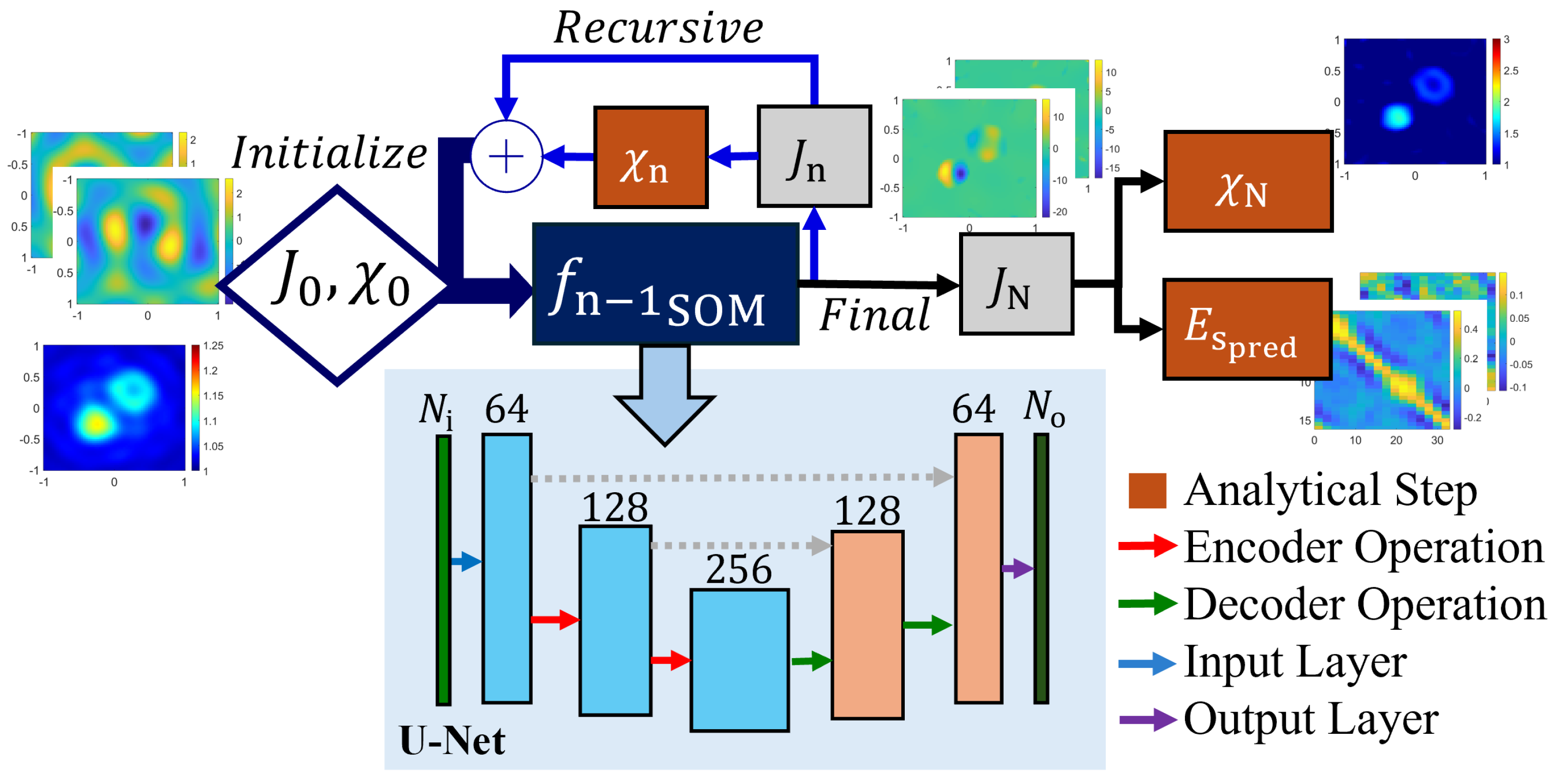
6. Conclusions

Multi-fidelity surrogate modeling offers a unique solution to the data-intensive demands of EM-based machine learning methods. This review comprehensively examined current MF surrogate modeling schemes for solving the forward and inverse problems. Notably, emphasizing how these MF methods enhance a model’s accuracy while reducing training data requirements. This review explored conventional and physics-based approaches for generating low-fidelity models, discussing their challenges and limitations. Additionally, the review covered key machine learning concepts, including data representation and model selection. Finally, promising research directions for advancing MF modeling were identified. This work will serve as a valuable resource for researchers aiming to apply machine learning algorithms to electromagnetic problems.