Design of Multimodal Obstacle Avoidance Algorithm Based on Deep Reinforcement Learning

Abstract

The navigation obstacle avoidance method based on deep reinforcement learning has stronger adaptability and better performance compared to traditional algorithms in complex unknown dynamic environments, and has been widely developed and applied. However, when using multimodal information input, deep reinforcement learning strategy networks extract features that differ significantly between simulated and real world environments, resulting in poor algorithm output strategies and difficulty in transferring models obtained from simulation training to actual environments. To address the aforementioned issues, this article utilizes image segmentation to narrow the gap in environmental features, integrates multimodal information, and designs a deep reinforcement learning multimodal local obstacle avoidance algorithm, MMSEG-PPO, based on proximal strategy optimization algorithms. The algorithm is then ported to practical environments for deployment and testing. The experiment shows that the algorithm proposed in this article reduces the gap between the simulation environment and the actual environment, and has better performance and generalization when transplanted to the real world environment.

1. Introduction

Autonomous navigation and obstacle avoidance are the foundation for achieving the intelligent control and safe travel of mobile robots. In complex real world environments, the agent needs to perceive the surrounding environment and its state through sensors, enabling it to make reasonable decisions in dynamic situations, quickly search for an optimal obstacle avoidance path between the starting point and the target location, and execute it [1]. In scenarios such as indoor services and intelligent delivery, mobile robots need to navigate through crowds and obstacles, avoiding collisions with pedestrians or obstruction of their paths. They may also need to interact with humans and adjust their routes and actions based on their movements and instructions, which introduces a more complex dynamic environment and requires unmanned platforms to have a certain level of adaptability to cope with environmental changes. To address this issue, deep reinforcement learning (DRL) algorithms can be employed to solve the motion planning problem of unmanned platforms in complex dynamic environments: deep learning is used to process high-dimensional sensor information, while reinforcement learning is used for decision making and planning.

In the real world, the environment that machines face is complex and ever-changing. A single sensor cannot meet the demand for diverse information and is easily affected by environmental factors, which limits the improvement of obstacle avoidance performance. By utilizing multiple sensors to acquire multimodal information and fusing them, it is possible to achieve completeness in perception under complex conditions, thereby enhancing the performance and adaptability of the algorithms. However, there is an unavoidable gap between simulation environments and real world environments, such as differences in object textures and lighting, which makes it difficult for algorithms trained in simulation environments to perform accurately in the real world. This reduces the generalization of the algorithms and limits the application of reinforcement learning from simulation to real world scenarios.

To address the above issues, this paper designs a DRL multimodal local obstacle avoidance algorithm MMSEG-PPO, based on the PPO algorithm. The approach involves incorporating multi-sensor data to extract environmental features as inputs for the decision-making algorithm. The main contributions are as follows:

(1). Image segmentation technology is utilized to reduce interference from shadows, lighting, textures, and other factors in the images, thus narrowing the gap between reality and simulation. The images captured by the camera are segmented into three binary maps: passable areas, general obstacles, and critical obstacles, providing a comprehensive representation of the environment. This effectively addresses the significant difference between reality and simulation of the algorithm, allowing the model to be better deployed from the simulation environment to the real world environment.

(2). A reward function is designed to reflect complex obstacle avoidance rules, guiding the robot to avoid obstacles and reach the target point, thereby overcoming the issue of sparse rewards during the training process.

(3). Curriculum learning is employed to decompose complex tasks into subtasks with progressively increasing difficulty, enabling the robot to gradually understand the behavioral patterns required for the tasks, reducing local convergence, and accelerating the training process.

(4). Deployment and comparative experiments are conducted in real world environments.

2. Related Work

Path planning requires the consideration of environmental information, which often involves large volumes of data with high dimensionality, posing challenges for traditional reinforcement learning. The feature extraction capabilities of deep reinforcement learning networks effectively address the dimensionality issues encountered by conventional reinforcement learning. The input of perceptual information into deep reinforcement learning algorithms undergoes a progressive enhancement in complexity.

Positional information is one of the simplest types of input data, which is why, in early research on deep reinforcement learning for path planning, algorithms commonly used grid maps, target location, obstacle information, and the robot’s location as state inputs. In recent research, these inputs are often stacked with other features to serve as the state input for reinforcement learning. LiDAR is a sensor widely used in mobile robots due to its simplicity and the minimal difference in data between simulation and real world environments. Ma et al. [2] converted LiDAR information into logarithmic map data, allowing for more pixel representation of the area close to the robot. The algorithm employed distributed proximal policy optimization (DPPO) to train a neural network, using three frames of logarithmic maps through three convolutional layers for feature extraction. The network’s fully connected output generated a 2D vector representing the continuous action space, ultimately achieving obstacle avoidance in complex multi-robot scenarios without the need for communication.

In addition to LiDAR, images are also frequently used as inputs for DRL algorithms, including standard RGB images and depth images containing depth information. Ding et al. [3] proposed an obstacle avoidance algorithm using a monocular camera, where RGB images were converted into pseudo-LiDAR information containing depth and semantic data. This enabled the algorithm to handle irregularly shaped and special material obstacles that traditional LiDAR struggles with, ultimately achieving obstacle avoidance for mobile robots with an Actor–Critic framework. To address the limited field of view of a single camera, Huang et al. [4] employed multiple cameras to capture information from various directions and used an attention mechanism to reduce information redundancy. Additionally, to facilitate the transfer from simulation to reality, they reduced the dimensionality of RGB images into boundary line networks, significantly lowering the complexity of the DRL framework and the policy search space. Barron T et al. [5] used RGB images as input for a DQN, training the robot to complete complex tasks and achieving better performance than depth images. Tai et al. [6] used depth images as input to a Q-network, outputting the mobile robot’s actions and velocities, and trained the Turtlebot robot to avoid walls in an indoor corridor (forward, right, left). The navigation performance was verified in various 3D simulated environments, enabling motion planning for mobile robots in scenarios with multiple static obstacles. Wang et al. [7] utilized depth image information to transfer learned navigation policies to unknown environments via feature inheritance, achieving the transfer of robot navigation strategies from simulation to reality using DQN.

A single sensor may encounter common issues such as insufficient sampling efficiency, delayed real-time feedback, and a lack of environmental information. By fusing data from multiple sensors, multimodal information from various sensors can achieve comprehensive perception in complex situations, thereby improving the performance and adaptability of algorithms. Consequently, multimodal DRL algorithms have been extensively studied in recent years. Srouji et al. [8] combined LiDAR and ultrasonic sensor scan data to detect a wider range of obstacle types. They integrated the Dynamic Window Approach (DWA) algorithm with an automatic emergency intervention collision system, enabling reinforcement learning to safely operate in real world environments. Both Tan [9] and Huang [10] focused on the fusion of LiDAR and camera image data. Tan et al. designed a lightweight multimodal data fusion network that integrated LiDAR and image data, along with vehicle motion information derived from odometry feedback, providing more complete environmental and vehicle motion information for subsequent policy modules. Additionally, they utilized an artificial potential field to construct the reward function for the DDPG algorithm, achieving faster convergence and higher success rates. Huang used raw RGB images as input and fused them with LiDAR data, employing modality separation learning and curriculum learning paradigms to accelerate training. Khalil [11] processed image information to obtain range views and residual maps, which were then handled by a real-time multimodal fusion network, LicaNext. Subsequently, a single LiDAR sensor was used to construct a bird’s-eye view of the environment, with the processed images being fed into a DRL algorithm to learn end-to-end driving policies, demonstrating the effectiveness of the method across various environments and changing weather conditions. Zhou et al. [12] combined vehicle IMU data, local point cloud images, and front camera observation images, designing specific feature extraction networks for each modality and using modality separation learning to effectively train the entire DDQN model. They also introduced semantic segmentation to preliminarily extract front camera observation data, enhancing learning efficiency and ultimately achieving the safe navigation of unmanned vehicles over complex and rugged terrain in outdoor environments. Chen et al. [13] proposed a Multimodal State Space Model (MSSM) capable of representing complex dynamics and multimodal observations, and employed MuMMI training loss to encourage the sharing of a common latent space among modalities, providing a novel and robust self-supervised reinforcement learning method for multi-sensor integration. Li et al. [14] fused the multimodal distribution probabilities of surrounding vehicles to establish a multimodal driving risk field in dynamic collision zones. The algorithm utilized the Recurrent Deterministic Policy Gradient (RDPG) algorithm, which enhanced the current observation state and combined it with previous states, allowing it to find the optimal driving strategy under partially observable conditions.

In summary, deep reinforcement learning enables the selection of appropriate actions based on the current sensor input without relying on labels or maps. Different algorithms and their variants each have advantages when addressing specific problems. Value-based deep reinforcement learning, such as DQN, is better suited for handling discrete action spaces, while policy-based deep reinforcement learning algorithms can output continuous action spaces, making them more suitable for end-to-end navigation and obstacle avoidance on unmanned platforms. As the complexity of the environment increases, environmental features have evolved from simple positional information to multimodal information that integrates data from multiple sensors such as LiDAR and cameras. The methods of feature processing have also evolved from simple feature stacking to incorporating techniques such as LSTM, convolutional neural networks, and image segmentation. As task complexity increases and task environments become more diverse, the exploration of multimodal deep reinforcement learning algorithms for path planning has emerged as a predominant trend in research. Compared with the prior algorithm with single-input LiDAR data or image data, the camera is relatively limited by ambient light, and the LiDAR can still maintain stable work at night or in low-light conditions. The LiDAR can obtain the precise position of the object by firing the laser pulse and measuring its reflection time, while the camera can identify and classify the object through image processing technology. The method combining image and LiDAR data can better extract environmental features and improve the speed of training convergence.

3. Algorithm Implementation

3.1. MMSEG-PPO Design of Local Obstacle Avoidance Algorithms

Based on the principles of reinforcement learning, the obstacle avoidance task of a mobile robot can be viewed as a Markov Decision Process (MDP) problem, where the agent continuously optimizes its policy through interaction with the environment. In this context, it is essential to define the state space, action space, and reward function for the mobile robot agent. The algorithm is divided into two modules: a multimodal information feature extraction module and an autonomous obstacle avoidance decision-making module. In the first module, the sensory information, including the robot’s state information, image perception data, and LiDAR data, undergoes preliminary feature processing. By employing image semantic segmentation, the discrepancy between the simulation and reality is reduced, thereby facilitating better transfer from simulation to real world scenarios. In the second module, the processed information is fed into a policy network, which ultimately outputs the linear and angular velocities that control the robot’s movement. Additionally, curriculum learning is utilized to accelerate training and enhance the generalization capability of the resulting model. The proposed algorithm framework is illustrated in Figure 1.

3.2. Reinforcement Learning

(1) State Space

The mobile robot is equipped with sensors such as an IMU, depth camera, and LiDAR to collect information about both itself and the environment. In this paper, the state space $S_t$ for reinforcement learning includes processed LiDAR data $S_{t\_laser}$, segmented image information $S_{t\_image}$, and the robot’s state information $S_{t\_robot}$. These processed features will be input into the policy network to generate the corresponding actions. The specific methods for processing this information will be detailed in Section 3.3.

(2) Reward Function

The reward function defines the reward values that the mobile robot receives from the environment after performing different actions. These rewards reflect the rules that the robot needs to follow during obstacle avoidance and are a crucial factor influencing the convergence speed of the algorithm, guiding the robot towards the target point while avoiding obstacles. Previous work often designed reward functions based solely on positional information. While this approach is simple, in real world environments the robot needs to consider multiple aspects during the obstacle avoidance process, including its orientation, obstacle avoidance strategies, and reaching the target point via the shortest path. The reward function scheme designed in this paper is as follows [15]:

Arrival Reward $R_{target}$: When the robot reaches the vicinity of the target point, it is given an arrival reward, and the environment is reset to start the next round of training. The distance between the robot’s center point and the target point is denoted as $d_t$, and $\lambda$ represents the predefined arrival threshold. If $d_t$ is less than $\lambda$, the robot is considered to have reached the target point.

$$R_{target}=500,\mathrm{if}{\mathrm{d}}_t<\lambda$$

(1)

Collision Penalty $R_{collision}$: When the robot collides with an obstacle, it is given a collision penalty, and the environment is reset to start the next round of training. During the simulation, $min(laser\_dat{a}_t)$ represents the minimum value of the LiDAR scan data. If ${\eta }_c$ falls below the collision threshold, a collision is considered to have occurred.

$$R_{collision}=-500,\mathrm{if}min(laser\_dat{a}_t)<{\eta }_c$$

(2)

Obstacle Avoidance Penalty $R_{avoidance}$: To reduce the occurrence of collisions, we aim for the robot to maintain a safe distance from obstacles ${\eta }_a$. Therefore, an obstacle avoidance threshold is set, with a lower limit of ${\eta }_{ad}$ and an upper limit of ${\eta }_{au}$. When the minimum LiDAR value falls within the ranges ${\eta }_c$, ${\eta }_{ad}$, and ${\eta }_{au}$, different levels of obstacle avoidance penalties are assigned accordingly.

$$\left\{\begin{array}{c}{R}_{avoidance}=-0.5·(1/min(laser\_dat{a}_t)),{\eta }_{ad}<min(laser\_dat{a}_t)<{\eta }_{au}\hfill \\ R_{avoidance}=-2,min(laser\_dat{a}_t)<{\eta }_{ad}\hfill \\ R_{avoidance}=0,{\eta }_{au}<min(laser\_dat{a}_t)\hfill \end{array}\right.$$

(3)

Orientation Reward $R_{heading}$: To encourage the robot to move towards the target point, an orientation reward is given. The deviation angle $\theta$ between the robot and the target point is used for this purpose. If $\theta$ is within a given orientation threshold, the robot is considered to be moving towards the target point.

$$\left\{\begin{array}{c}{R}_{heading}=0.5,-1<\theta <1\hfill \\ R_{heading}=-0.5,\mathrm{else}\hfill \end{array}\right.$$

(4)

Distance Reward $R_{goal}$: In addition to the direction of travel, the distance between the robot and the target point is also an indicator of whether the robot is moving towards the target. However, since there is no definite range between the two, this paper uses the interval distance ${\delta }_t$ between two steps to provide a reward, where $Cr$ is a constant greater than 0.

$$R_{goal}=Cr\ast {\delta }_t$$

(5)

Traversal Reward $R_{drive}$: In the early stages of training, it is common for the policy to output angular velocity for extended periods, causing the robot to spin in place. Therefore, a traversal reward is set to encourage changes in the robot’s linear velocity and to reduce changes in angular velocity. Here, $A_{vt}$ represents the linear velocity action at time t, and $A_{\omega t}$ represents the angular velocity action at time t.

$$R_{drive}=A_{vt}-A_{\omega t}$$

(6)

Time Penalty $R_{\mathrm{time}}$: During the training process, the path taken by the robot to reach the target location may not be the shortest. Therefore, a fixed time penalty is imposed at each step to encourage the robot to tend towards reaching the target point via the shortest path.

$$R_{time}=-0.1$$

(7)

The aforementioned rewards collectively form the reward function during the reinforcement learning training process, as shown in Equation (8). The calculated reward values will be added to the reinforcement learning quadruple as experience to be stored and used for the iterative training of the algorithm parameters [16].

$$R_{target}=R_{collision}+R_{avoidance}+R_{heading}+R_{goal}+R_{time}$$

(8)

(3) Action Space

In real world environments, the output of mobile robots consists of continuous linear and angular velocities. The range of linear velocity is [0, 1] meters per second (since the actual robot’s maximum speed is 0.8 m per second, the output results will be scaled proportionally), and the range of angular velocity is [−1, 1] radians per second. The robot is controlled based on ROS (Robot Operating System). When the DRL (Deep Reinforcement Learning) algorithm provides an action output, it will be transmitted using the Twist standard message in ROS. As the control method for both simulation and actual robots is a four-wheel differential drive, they are capable of turning in place. Therefore, the x-axis linear velocity in the Twist message is set to the value of $A_{vt}$ and the z-axis angular velocity is set to the value of $A_{\omega t}$. Once the message is sent to the robot’s underlying velocity controller, the robot will be able to travel at the given velocities.

(4) Parameter Settings

The general parameters of the algorithm are shown in

Table 1. General parameter settings of the algorithm.

Parameter	Parameter Size	Meaning
max_steps	3,000,000	Maximum Number of Steps in the Training Process
max_ep_steps	2000	Maximum Number of Steps Per Episode During Training
update_timestep	10,000	Update Interval for Policy Parameters
K_epochs	80	Number of Episodes Per Policy Update
batch_size	64	Data Volume Per Parameter Update
gamma	0.99	Discount Factor for Future Rewards
eps_clip	0.2	Clipping Boundary in PPO Algorithm
lr_actor	0.0003	Learning Rate of the Actor Network
lr_critic	0.001	Learning Rate of the Critic Network
expl_noise	0.1	Exploration Noise Variance

.

Parameters such as gamma and eps_clip are set according to the recommended values for the PPO algorithm in the relevant literature. For example, gamma = 0.99 is usually used for long-term reward calculations and has good convergence; eps_clip = 0.2 balances the stability of policy updates with the ability to explore. Experiments with eps_clip adjusted to 0.1 and 0.3 showed that a smaller clipping value (e.g., 0.1) could result in insufficient policy updates, while a larger value (e.g., 0.3) would increase the volatility of the strategy. For the batch_size and K_epochs parameters, smaller batch_size and larger K_epochs increase the training time, but may improve the stability of the policy. It is found that the increasement of lr_actor from 0.0003 to 0.001 will accelerate the convergence of the model in the initial stage but reduce the long-term stability. A reduction to 0.0001 may result in slow convergence. We tried several parameter combinations in a small-scale experiment and, by observing the training convergence speed, the performance of the final strategy, and the learning stability, we finally selected the current parameter configuration, which is the optimal compromise between stability and performance.

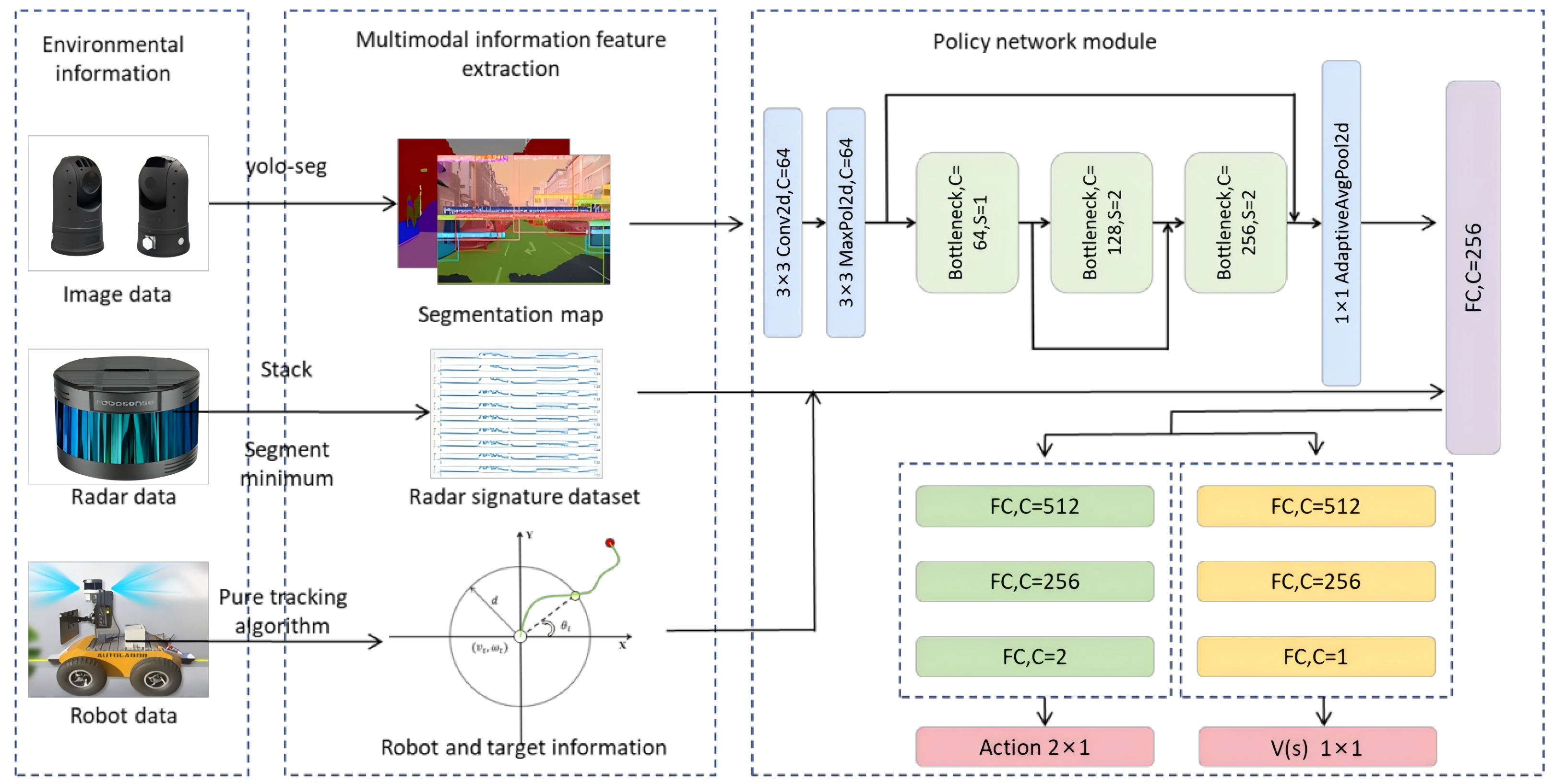
3.3. Multimodal Feature Extraction Module

3.3.1. Robot’s Self-State Information Processing

The robot’s self-state can be derived from the robot’s position $(x_{robot},y_{robot})$, velocity $(v_t,{\omega }_t)$, and position of the target point $(x_{goal},y_{goal})$, and its specific representation is shown in Figure 2.

Among these, each data point uses the odom frame as the reference coordinate system. By collecting the positions of the robot and the target point at time t, the distance between the robot and the target point $d_t$, as well as the deviation angle between the robot and the target point ${\theta }_t$, can be calculated, thereby describing the orientation towards the target point. By collecting the robot’s linear velocities $v_t$ and angular velocities ${\omega }_t$ at the current time, the movement of the robot can be described. Ultimately, the robot’s self-state information $S_{t\_robot}$ is recorded as follows.

$$S_{t\_robot}=(d_t,{\theta }_t,v_t,{\omega }_t)$$

(9)

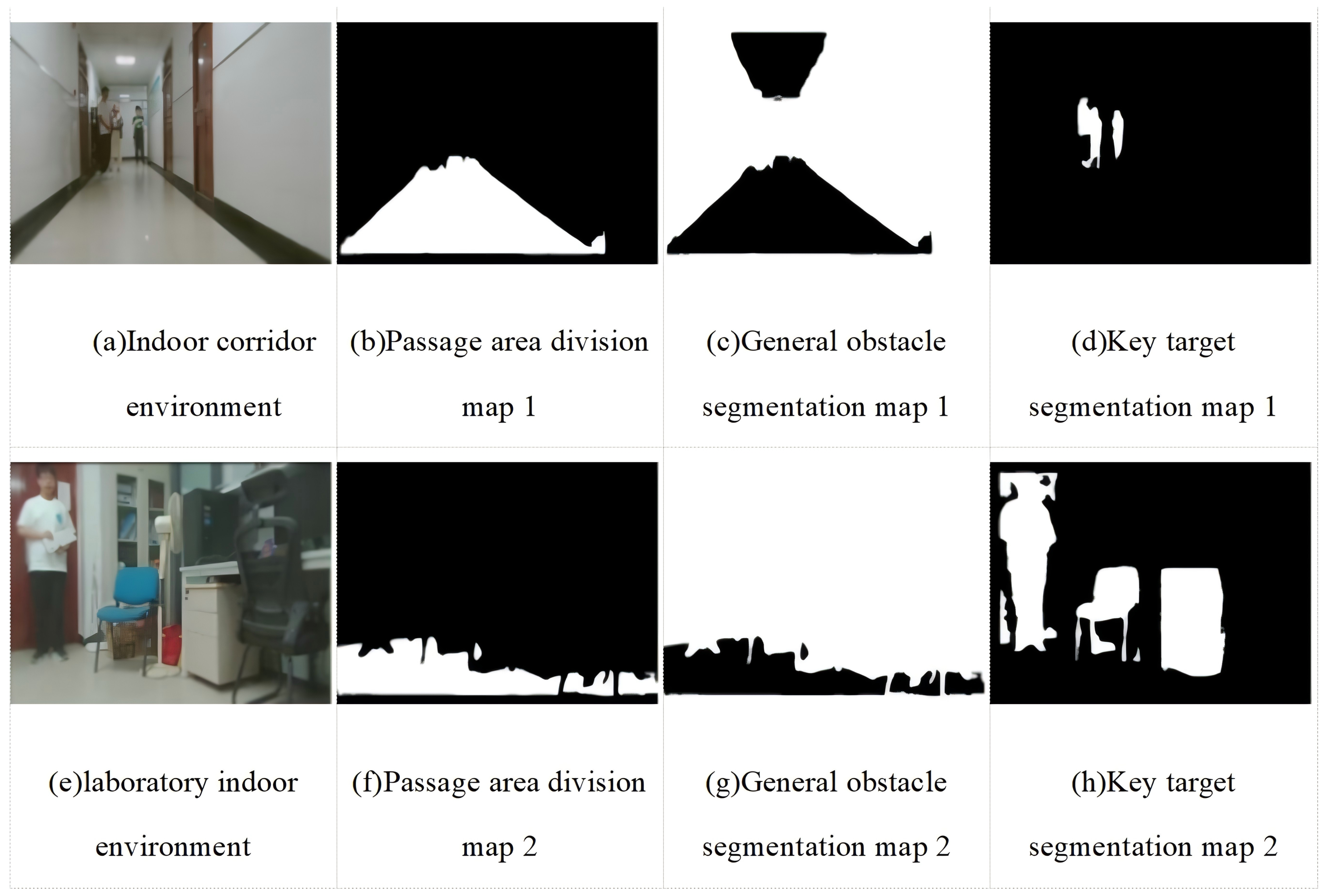
3.3.2. Visual Image Perception Information Processing

Due to factors such as lighting conditions and sensor characteristics, differences between real and simulated environments are inevitable. When RGB images are directly used as input for deep reinforcement learning, the extracted features often do not correspond well with real world scenarios, leading to poor performance when the algorithm is deployed in real environments. To address this issue and facilitate the transfer from simulation to reality, this study employs image segmentation as a preprocessing step. By segmenting the images captured by the camera and using the segmented images as input, interference factors in the images, such as shadows, lighting, and textures, can be effectively ignored. This method helps to eliminate the discrepancies between real and simulated environments, thereby enhancing the generalization capability of the algorithm from simulation to reality.

To ensure the processing speed when deployed on edge devices, this study utilizes a Yolov5s-based framework for image segmentation. Yolov5 is a lightweight network model that maintains high accuracy while requiring relatively low computational resources, making it suitable for deployment on edge devices with limited computational power. Yolov5s-seg extends this framework by adding a segmentation head, enabling the model to output pixel-level segmentation maps. Through segmentation, objects in the image, such as pedestrians, vehicles, and obstacles, can be distinguished from the background, allowing the identification of obstacles (e.g., pedestrians) in the region ahead. Additionally, the Yolov5s framework can be used for image recognition, allowing the identification of segmented objects and providing class labels for them.

In this study, the segmented images will be processed into three types of segmentation maps based on the segmentation labels: first, a binary segmentation map of navigable and non-navigable areas, $S_{seg1}$, which separates the navigable region from other background areas, indicating whether the path ahead is passable; second, a binary segmentation map for common obstacles, $S_{seg2}$, which distinguishes common obstacles such as walls from the navigable area, representing the obstacle conditions ahead; third, a binary segmentation map for key objects of interest, $S_{seg3}$, which separates objects like pedestrians and furniture from the background, indicating obstacles that require special attention. The segmented images $S_{seg1}$, $S_{seg2}$, and $S_{seg3}$ will be used as input states and fed into the subsequent policy network. The segmentation results are shown in Figure 3.

3.3.3. LiDAR Perception Data Processing

The data from LiDAR are relatively similar under real world and simulation conditions, with simple data features, and they are widely used in navigation and obstacle avoidance algorithms. In this paper, a model LD19 2D LiDAR is used, which is capable of measuring the distance and angle of obstacles. Typically, the number of points scanned by the LiDAR is set to an integer multiple of 180. However, in practical use, the actual number of scanning points of the LiDAR fluctuates between 448 and 452, and it may be set to NaN due to environmental material reasons, causing the LiDAR to fail to receive information. Since the input dimensions of the neural network need to be strictly fixed and cannot be NaN or Inf, and in order to reduce the input feature dimensions of the decision-making module, this paper will perform manual feature processing on the LiDAR perception information.

In this paper, the detection range of the LiDAR is 180° in front, with a detection distance of [0.02 m, 12 m]. Firstly, the NaN and Inf values in the processed data are addressed by replacing Inf with the maximum value of 12 and NaN with the average of the surrounding 10 non-NaN values, to ensure data correctness. Subsequently, the 180 field of view is divided into 20 regions, and the minimum value of the data within these 20 regions is calculated. The data from three consecutive time steps are averaged, and the averaged 20 minimum values are stored in the laser_data array, serving as the features obtained from the radar data, which are noted as the LiDAR state information $S_{laser}$. The Robot LiDAR information processing is shown in Figure 4.

3.4. Multimodal Feature Extraction Module

In this section, a policy module that integrates feature extraction and the Actor–Critic network is constructed to process and interpret the multimodal sensory data. After the sensory information is processed as described in Section 3.2, it is input into the policy network module. The specific network structure is shown in Section 3.1. This includes an image feature extraction network, where the three segmented images are input into the feature extraction network for further feature extraction. The semantic segmentation maps used here are directly obtained from the preceding image segmentation module and do not require parameter updates from reinforcement learning training. The semantic segmentation maps can segment various object classes, such as pedestrians and vehicles. Before input, they are transformed into three binary images, which represent the obstacle features (especially pedestrians) in the forward area from multiple perspectives, thereby enabling the agent to make better decisions.

The image features will first undergo an elementary feature extraction through a 3 × 3 convolutional layer; subsequently, max pooling is applied to reduce spatial dimensions, decrease computation, and avoid overfitting; then, the features will enter three Bottleneck blocks for deep extraction, each Bottleneck containing convolutional layers and residual connections to prevent gradient vanishing; finally, the features are further compressed through a pooling layer. The compressed features will be stacked and fused with the LiDAR features and the robot’s self-state features, and then passed through a fully connected layer to output an intermediate feature of 256 dimensions. This intermediate feature will then be input into the Actor and Critic modules. The Actor module contains three fully connected layers, activated by the ReLU function, with the output being the linear and angular velocities for controlling the robot’s movement. The Critic module also contains three fully connected layers, but the final output dimension is 1, which is the value assessment of the current state.

3.5. Curriculum Learning

Curriculum learning is a heuristic learning process inspired by the way humans and animals learn, progressing from simple to complex tasks. Solving easier problems first helps the model establish a foundational knowledge framework, enabling it to better handle more complex problems later on. In deep reinforcement learning training, complex environments and tasks often cause the agent to get stuck in local optima. Introducing curriculum learning can enhance the model’s learning efficiency and overall performance. The goal of this study is to enable a mobile robot to navigate in a complex dynamic environment, avoiding pedestrians and other obstacles while ultimately reaching the target point. Directly adding numerous dynamic obstacles in the simulation environment would make training exceedingly difficult. Therefore, we adopt a curriculum learning approach, dividing the training into two stages. The two−stage simulation training environment is shown in Figure 5.

In the first stage of training, the robot is trained in a small area with fewer static obstacles, with the robot’s starting point being a random location on the map that does not collide with obstacles. The environment is reset after the robot reaches the target point or collides with an obstacle. This stage is primarily used to train the robot’s ability to avoid static obstacles and search for the target.

In the second stage of training, the environment is augmented with both static obstacles and dynamically walking pedestrians to train the robot’s ability to avoid dynamic obstacles. At this point, instead of immediately resetting the environment after the robot reaches the target point, only the position of the target point is changed, while the robot’s position remains the same. This allows the robot to acquire the capability of navigating to multiple consecutive target points on the map.

By using the approach of curriculum learning, the complexity of initial learning can be reduced, allowing the model to quickly overcome the period of difficulty in obtaining sufficient rewards early on and to reduce local convergence in simple tasks. At the same time, through gradual learning, the model can gradually build and refine its understanding of complex concepts, achieving better performance than a one-time training approach. However, it is important to note that, in the initial training process, if a small number of static obstacles are not set and the ability to reach the target point is only trained in a limited-range scenario, it may lead to the model being unable to extract sufficient features from the environmental information, resulting in the inability to obtain a strategy that meets the requirements.

4. Experiment and Analysis

4.1. Simulation Experiment and Analysis of Multimodal Deep Reinforcement Learning for Local Obstacle Avoidance

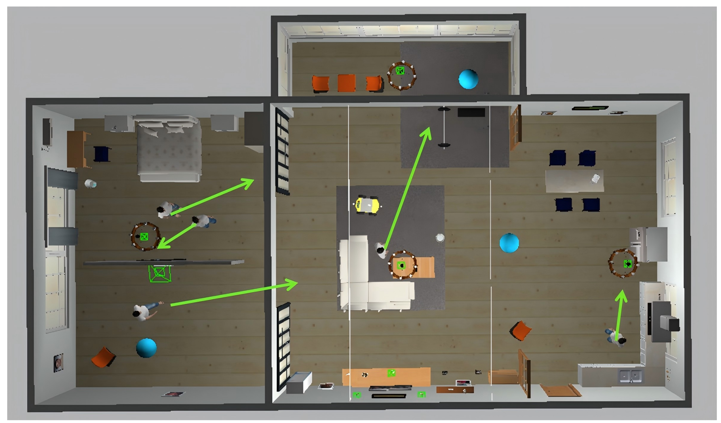
4.1.1. Training Environment and Parameter Configuration

The training scenarios for this study were constructed using Gazebo, creating an indoor simulation environment. First is the static simulation environment, which measures 10 m × 20 m and includes basic obstacles such as bookshelves and sofas. The environment is set with 3–5 chairs and toys as random obstacles, whose positions vary randomly within a certain range. The starting position of the robot and the location of the target point are both random points that do not collide with obstacles, with a random starting angle. In the dynamic simulation environment, all other conditions remain the same, but pedestrians move within the scene along certain trajectories. The scene is depicted in Figure 6, where the green arrows indicate the direction and position of movement, which is based on the core simulation behavior of Pedsim.

After the training environment is set up, the obstacle avoidance training is conducted on the algorithm proposed in this paper. The basic parameter settings for the PPO algorithm used in this paper are shown in Table 1.

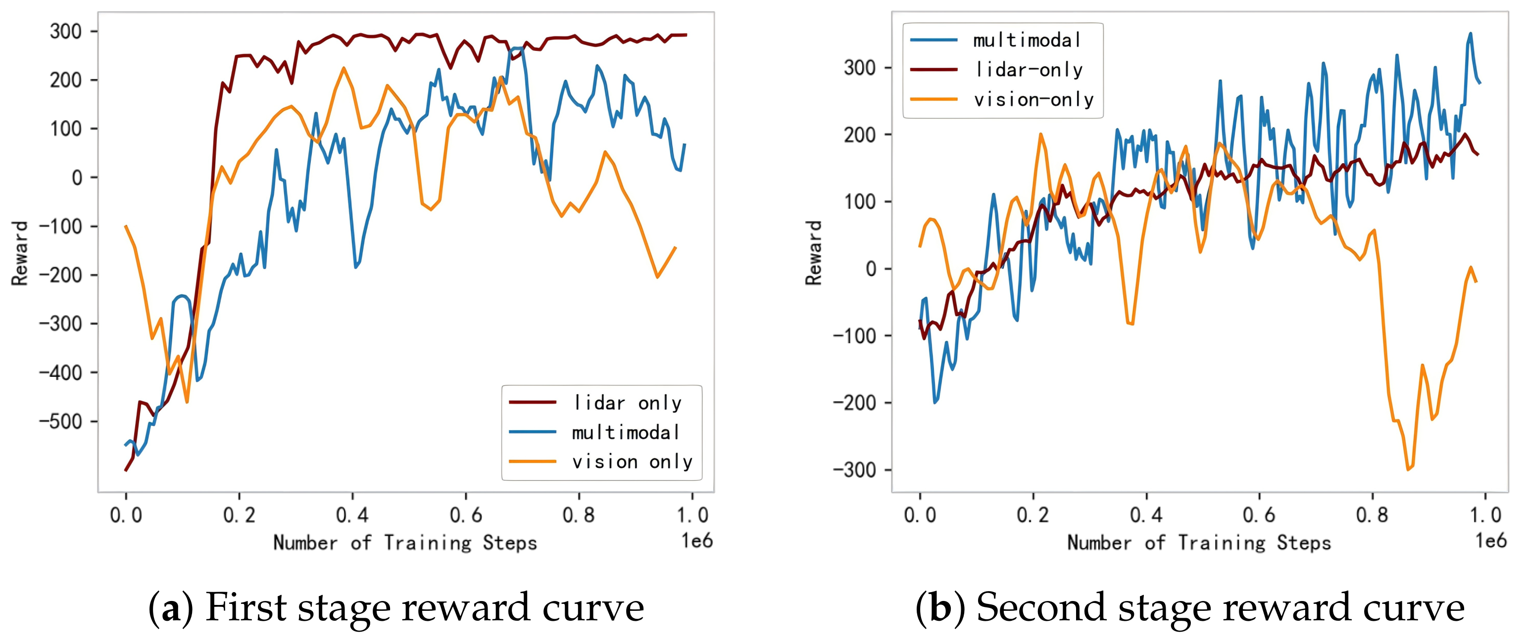
4.1.2. Algorithm Training Experiment and Analysis

In this section, the PPO algorithm is used for multimodal fusion training, comparing the reward curves of using LiDAR data only, segmented image data only, and the multimodal fusion algorithm proposed in this paper, in addition to the robot’s state information. Using the curriculum learning approach, in the first phase, the training environment only contains static obstacles. The training results are shown in Figure 7a.

From the comparison chart, it shows that the method using LiDAR only has the fastest training speed and achieves the highest reward value. When using images only, the convergence is poor and the training may even fail eventually. With the multimodal perception method, the curve shows a steady improvement in the early stages, and the final reward value obtained is higher than that of using images only, with better convergence. This may be due to the stable performance of LiDAR data in the simulation process, while the input image data undergoes continuous image segmentation operations, and the obtained input states are closely related to the effectiveness of the segmentation model. When using multimodal data, the feature dimension of the input is higher, which makes it more difficult for the model to converge.

Adopting the concept of curriculum learning, the model that has reached convergence in the first phase is selected and applied to the dynamic obstacle avoidance environment for the second phase of training. The training environment includes both static obstacles and dynamic pedestrian obstacles. The training results are shown in Figure 7b.

The reward curve fluctuation of the reinforcement learning navigation obstacle avoidance algorithm is caused by many factors: (1). The balance of exploration and utilization: At the beginning of learning, the algorithm may perform a lot of exploration, which can lead to fluctuations in the reward curve, as random actions can bring unpredictable results. (2). The uncertainty of environment: Obstacles, targets, and other factors in a dynamic environment can change over time, resulting in different rewards even if the algorithm takes the same action. (3). The instability of strategy: In reinforcement learning, strategies are updated based on the current sample. If the sample is noisy or the sample size is insufficient, the strategy may change significantly with each update, causing the reward curve to fluctuate. (4). The trade-off between long-term and short-term rewards: In the same navigation task, the algorithm needs the trade-off between the instant rewards and long-term rewards. This trade-off can cause strategies to look unstable in the short term, causing fluctuations in the reward curve.

The figure shows that the cumulative reward value initially drops sharply, with the reward value at the starting point of training being about −100, which is a significant improvement compared to the first phase. This indicates that, at this point, some obstacle avoidance experience has already been acquired. As the number of training steps increases, the reward value gradually improves and stabilizes, but the final converged reward value is lower than that of the first phase. When using visual images only, the reward still fluctuates greatly and it is difficult for it to converge, and it rapidly decreases around $8\times {10}^5$ steps. When using the multimodal algorithm proposed in this paper, the highest final reward value is obtained. This demonstrates that, in dynamic environments, the multimodal algorithm can achieve better results. Starting from initially only being able to avoid static obstacles, it gradually becomes capable of evading dynamic pedestrian obstacles and reaching the target point. An example of its driving trajectory in the simulation environment is shown in Figure 8.

4.1.3. Testing and Analysis of the Algorithm’s Obstacle Avoidance Effectiveness

After the algorithm training is completed, the performance of the trained model is evaluated through testing. The testing environments are divided into two: the indoor room simulation environment and the indoor lobby simulation environment. Each environment is tested under static scenarios as well as scenarios with dynamic pedestrians. During testing, the initial position of the mobile robot and the location of the target point are randomized. The specific parameters for each scenario are detailed in

Table 2. Test scenario parameter settings.

Environment	Environment Size	Number of Static Obstacles	Dynamic Number of Pedestrians
indoor room environment	9 m × 12 m	3–4	3–4
indoor hall environment	25 m × 30 m	5–6	10–20

.

In this experiment, the following baseline methods are selected for comparison with our method:

(1) GD-RL [17]: This is a depth reinforcement learning obstacle avoidance method using LiDAR, which calculates points of interest from radar data and uses them as features for the optimal navigation path, guiding the robot towards the final target point and achieving goal-driven exploration navigation.

(2) MCB-DRL [3]: This is a depth reinforcement learning obstacle avoidance method based on monocular camera images, which converts RGB images into pseudo-laser measurements, enabling efficient reinforcement learning training and effective path planning.

(3) LiDAR-only: This is an ablated version of our method, which uses only robot information and LiDAR data as state input.

(4) Vision-only: This is another ablated version of our method, which uses only robot information and segmented image information as input.

Each algorithm was tested 100 times in the corresponding scenarios, and the number of successful attempts, instances of getting lost, and collision occurrences were statistically recorded for each method under different environments. The collected data are presented in

Table 3. Obstacle avoidance test results in simulation environment.

Scene	Algorithm	Number of Successes	Number of Treks	Number of Collisions
indoor room environment (static)	GD-RL	78	8	14
	MCB-DRL	87	5	8
	LiDAR-only	85	5	10
	Vision-only	80	5	15
	Ours	91	0	9
indoor room environment (dynamic)	GD-RL	70	8	22
	MCB-DRL	81	6	13
	LiDAR-only	78	4	18
	Vision-only	77	5	18
	Ours	86	2	12
indoor hall environment (static)	GD-RL	83	5	12
	MCB-DRL	82	3	15
	LiDAR-only	79	3	18
	Vision-only	83	2	15
	Ours	88	1	11
indoor hall environment (dynamic)	GD-RL	78	2	20
	MCB-DRL	75	5	20
	LiDAR-only	70	4	26
	Vision-only	78	3	19
	Ours	83	3	14

. Figure 9 shows the trajectory of a mobile robot in an indoor scene during one of the test runs.

The analysis of the data in the table and the trajectories is as follows:

(1) As the size of the environment increases, the effectiveness of the model’s obstacle avoidance decreases. This is due to the increased distance between the target point and the robot as the environment size grows. In the training scenes, the distance between them is typically around 5 m. An excessively large distance value in the input state can significantly affect the model’s performance. It is also noted that the algorithm using LiDAR only is relatively more affected, which may be because, when the scene is too large, it may exceed the maximum range of the LiDAR (set to 12 m), and the data points become sparser, making it difficult for the model to obtain effective input features.

(2) The model is capable of moving towards the target point and effectively avoiding obstacles. The number of obstacles has a limited impact on the model’s effectiveness; it does not necessarily lead to worse performance; as long as there is sufficient passage distance between obstacles, the robot can navigate smoothly according to the strategy. However, in more cluttered environments, there is a certain degree of performance decline when using both LiDAR and image data. This may be due to the difficulty in extracting features from the cluttered information in the environment, and the limited field of view of the robot’s sensors, which makes it challenging to fully perceive the obstacle information in the environment, leading to collisions with obstacles at the middle part of the robot.

(3) In environments with dynamic pedestrians, the performance of the LiDAR-only method is poorer. This is mainly because, when using LiDAR, the robot typically scans only the lower part of pedestrians, resulting in fewer data points. In contrast, when using image data, the robot can fully capture the information of pedestrian obstacles, leading to better performance. However, when the pedestrians’ clothing color is similar to the environment background, it can also fail to segment and recognize the pedestrians, leading to obstacle avoidance failures.

The comprehensive obstacle avoidance success rate of the algorithm proposed in this paper is 89.5% in different static environments and 84.5% in dynamic scenarios, effectively realizing the local obstacle avoidance function of mobile robots. Compared with its ablation algorithm, the proposed algorithm performs better in all scenarios except for the static indoor room simulation environment, indicating that the use of multiple sensors can effectively mitigate the limitations of single sensors. The fluctuation of success rates in different scenarios is smaller compared to other baseline algorithms, with higher success rates, which demonstrates that the algorithm in this paper has stronger generalization and adaptability to various scenarios.

4.2. Multimodal Deep Reinforcement Learning for Local Obstacle Avoidance: Real Vehicle Experiment and Analysis

4.2.1. Model Deployment Process

To test the generalization of the algorithm proposed in this paper and demonstrate its ability to better facilitate the transition from simulation to reality, a mobile robot obstacle avoidance experiment was conducted. In this paper, the deployment of deep reinforcement learning algorithms is realized based on ROS. The mobile robot platform and the upper computer platform are within the same ROS local area network, with each algorithmic function implemented as a node. The specific process is shown in Figure 10. The environmental information is sensed and transformed into standard ROS messages for information transmission. After data processing, the data are used as input for the deep reinforcement learning-based obstacle avoidance decision-making model, and the resulting speed commands for controlling the robot’s movement are transmitted to the STM32 underlying driver of the chassis to control the motor’s rotation. The upper computer can receive node topic information within the system and display it in software such as Rviz and Rqt. It can also directly publish speed information to control the platform.

4.2.2. Real World Effectiveness Testing and Analysis

The trained algorithm model is imported into the decision-making model node as shown in the process depicted in Figure 10 to conduct the obstacle avoidance experiments. The experimental scenarios include an indoor laboratory setting and an indoor corridor setting. The dynamic pedestrian environment is simulated by actual human walking. The obstacle avoidance success rates of various algorithms in real world scenarios are compared, and the results are presented in

Table 4. Obstacle avoidance test results in actual environment.

Scene	Algorithm	Obstacle Avoidance Success Rate
Laboratory indoor environment (static)	GD-RL	66%
	MCB-DRL	72%
	LiDAR-only	68%
	Vision-only	63%
	Ours	79%
Laboratory indoor environment (dynamic)	GD-RL	62%
	MCB-DRL	61%
	LiDAR-only	55%
	Vision-only	46%
	Ours	76%
Corridor environment in the building (static)	GD-RL	65%
	MCB-DRL	75%
	LiDAR-only	70%
	Vision-only	68%
	Ours	82%
Corridor environment in the building (dynamic)	GD-RL	57%
	MCB-DRL	65%
	LiDAR-only	53%
	Vision-only	46%
	Ours	78%

. The driving effect in the corridor scenario is shown in Figure 11, with the yellow arrow indicating the direction of travel.

Observations from the experimental results reveal that the algorithm experiences a decline in obstacle avoidance efficacy when transitioning from a simulated environment to a real world setting. This decline is owing to the discrepancies in sensor data and the physical parameters of the robot’s movement between the simulated and actual environments. In practical settings, materials such as tiles, glass, and metal chairs in the laboratory can absorb or reflect laser beams, leading to inaccuracies in the laser data collected. When images are used as part of the input for reinforcement learning, any discrepancy between the training and real world environments can result in feature differences that affect the policy network’s output. The proposed algorithm achieved a comprehensive obstacle avoidance success rate of 81% in static scenarios and 77% in dynamic scenarios. By integrating LiDAR and visual information and utilizing image segmentation to abstract the images, the algorithm effectively mitigates the impact of various interferences in real world environments. As a result, the performance gap between the real world deployment and the simulation environment is relatively small. Nevertheless, the image segmentation process is also subject to real world environmental influences. In practice, there were instances where the algorithm failed to distinguish between walls and floors, leading to incorrect image segmentation. Hence, an effective segmentation model is essential for real world applications.

4.3. Summary of This Section

Experiments were conducted on the DRL-based multimodal local obstacle avoidance algorithm. The parameters of the simulation training environment were set, and the proposed algorithm, along with its ablated versions, were trained in two stages following a curriculum learning approach. The convergence of different algorithms was observed to demonstrate the feasibility of the algorithm proposed in this paper. The algorithms were tested in various environments to compare and analyze their navigation and obstacle avoidance success rates, collision rates, and other metrics, verifying the superiority and generalizability of the multimodal algorithm proposed in this paper to different scenarios. Subsequently, the trained models were deployed in real world environments, with the models implemented on a robotic experimental platform and tested in an actual corridor setting. The results showed that, in the simulation environment, the comprehensive obstacle avoidance success rate was 89.5% in static scenarios and 84.5% in dynamic scenarios; in the real world environment, the rates were 81% and 77% for static and dynamic scenarios, respectively. These rates are higher than those of the ablated algorithms and baseline algorithms, indicating that the algorithm proposed in this paper has better performance and transferability.

5. Results

In this paper, we design a DRL-based multimodal local obstacle avoidance algorithm, MMSEG-PPO, based on the PPO algorithm. We introduce multi-sensor data for the feature extraction of environmental information as input for the decision-making algorithm. Using image segmentation techniques, we reduce interference factors such as shadows, lighting, and textures in images, thereby decreasing the discrepancy between reality and simulation. The image information collected by the camera is segmented into three binary maps: traversable areas, general obstacles, and key focus obstacles, thus representing the surrounding environment from multiple aspects. On one hand, this paper employs a refined simulation environment to mimic a more realistic setting and, on the other hand, it utilizes image segmentation to ignore disruptive features, effectively addressing the issue of significant differences between the actual environment and the algorithm’s training environment. This allows the model to be better deployed from a simulation environment to a real world environment. The reward function is designed to reflect complex obstacle avoidance rules, guiding the robot to avoid obstacles and reach the target point, overcoming the sparse rewards problem during training. Curriculum learning is used to decompose complex tasks into progressively more difficult tasks, enabling the robot to understand the behavior patterns of the tasks from simple to complex, reduce local convergence, and accelerate the training process. The proposed algorithm achieves a comprehensive obstacle avoidance success rate of 89.5% in static scenarios and 84.5% in dynamic scenarios in simulation; in real world environments, the rates are 81% and 77% for the static and dynamic scenarios, respectively. Through ablation experiments and comparative experiments, we effectively validate the superiority of the multimodal perception algorithm over single-sensor information algorithms. Finally, the algorithm is deployed on a mobile robot in the real world using the ROS system for testing, demonstrating that the algorithm proposed in this paper can effectively transition from simulation to reality.

References

1. Farazi, N.P.; Zou, B.; Ahamed, T.; Barua, L. Deep reinforcement learning in transportation research: A review. Transp. Res. Interdiscip. Perspect. 2021, 11, 100425. [Google Scholar]
2. Ma, J.; Chen, G.; Jiang, P.; Zhang, Z.; Cao, J.; Zhang, J. Distributed multi-robot obstacle avoidance via logarithmic map-based deep reinforcement learning. In Proceedings of the Third International Conference on Artificial Intelligence and Computer Engineering (ICAICE 2022), Wuhan, China, 11–13 November 2022; SPIE: St Bellingham, WA, USA, 2023; Volume 12610, pp. 65–72. [Google Scholar]
3. Ding, J.; Gao, L.; Liu, W.; Piao, H.; Pan, J.; Du, Z.; Yang, X.; Yin, B. Monocular camera-based complex obstacle avoidance via efficient deep reinforcement learning. IEEE Trans. Circuits Syst. Video Technol. 2022, 33, 756–770. [Google Scholar] [CrossRef]
4. Huang, X.; Chen, W.; Zhang, W.; Song, R.; Cheng, J.; Li, Y. Autonomous multi-view navigation via deep reinforcement learning. In Proceedings of the 2021 IEEE International Conference on Robotics and Automation (ICRA), Xi’an, China, 30 May–5 June 2021; IEEE: New York, NY, USA, 2021; pp. 13798–13804. [Google Scholar]
5. Barron, T.; Whitehead, M.; Yeung, A. Deep reinforcement learning in a 3-d blockworld environment. In Proceedings of the IJCAI 2016 Workshop: Deep Reinforcement Learning: Frontiers and Challenges, New York, NY, USA, 11 July 2016; Volume 2016, p. 16. [Google Scholar]
6. Tai, L.; Paolo, G.; Liu, M. Virtual-to-real deep reinforcement learning: Continuous control of mobile robots for mapless navigation. In Proceedings of the 2017 IEEE/RSJ International Conference on Intelligent Robots and Systems (IROS), Vancouver, BC, Canada, 24–28 September 2017; IEEE: New York, NY, USA, 2017; pp. 31–36. [Google Scholar]
7. Wang, Y.; Sun, J.; He, H.; Sun, C. Deterministic policy gradient with integral compensator for robust quadrotor control. IEEE Trans. Syst. Man Cybern. Syst. 2019, 50, 3713–3725. [Google Scholar] [CrossRef]
8. Srouji, M.; Thomas, H.; Tsai, Y.H.H.; Farhadi, A.; Zhang, J. Safer: Safe collision avoidance using focused and efficient trajectory search with reinforcement learning. In Proceedings of the 2023 IEEE 19th International Conference on Automation Science and Engineering (CASE), Auckland, New Zealand, 26–30 August 2023; IEEE: New York, NY, USA, 2023; pp. 1–8. [Google Scholar]
9. Tan, J. A Method to Plan the Path of a Robot Utilizing Deep Reinforcement Learning and Multi-Sensory Information Fusion. Appl. Artif. Intell. 2023, 37, 2224996. [Google Scholar] [CrossRef]
10. Huang, X.; Deng, H.; Zhang, W.; Song, R.; Li, Y. Towards multi-modal perception-based navigation: A deep reinforcement learning method. IEEE Robot. Autom. Lett. 2021, 6, 4986–4993. [Google Scholar] [CrossRef]
11. Khalil, Y.H.; Mouftah, H.T. Exploiting multi-modal fusion for urban autonomous driving using latent deep reinforcement learning. IEEE Trans. Veh. Technol. 2022, 72, 2921–2935. [Google Scholar] [CrossRef]
12. Zhou, B.; Yi, J.; Zhang, X. Learning to navigate on the rough terrain: A multi-modal deep reinforcement learning approach. In Proceedings of the 2022 IEEE 4th International Conference on Power, Intelligent Computing and Systems (ICPICS), Shenyang, China, 29–31 July 2022; IEEE: New York, NY, USA, 2022; pp. 189–194. [Google Scholar]
13. Chen, K.; Lee, Y.; Soh, H. Multi-modal mutual information (mummi) training for robust self-supervised deep reinforcement learning. In Proceedings of the 2021 IEEE International Conference on Robotics and Automation (ICRA), Xi’an, China, 30 May–5 June 2021; IEEE: New York, NY, USA, 2021; pp. 4274–4280. [Google Scholar]
14. Li, L.; Zhao, W.; Wang, C. POMDP motion planning algorithm based on multi-modal driving intention. IEEE Trans. Intell. Veh. 2022, 8, 1777–1786. [Google Scholar] [CrossRef]
15. Li, K.; Xu, Y.; Wang, J.; Meng, M.Q.-H. SARL: Deep Reinforcement Learning based Human-Aware Navigation for Mobile Robot in Indoor Environments. In Proceedings of the 2019 IEEE International Conference on Robotics and Biomimetics (ROBIO), Dali, China, 6–8 December 2019; pp. 688–694. [Google Scholar]
16. Mackay, A.K.; Riazuelo, L.; Montano, L. RL-DOVS: Reinforcement Learning for Autonomous Robot Navigation in Dynamic Environments. Sensors 2022, 22, 3847. [Google Scholar] [CrossRef] [PubMed]
17. Cimurs, R.; Suh, I.H.; Lee, J.H. Goal-driven autonomous exploration through deep reinforcement learning. IEEE Robot. Autom. Lett. 2021, 7, 730–737. [Google Scholar] [CrossRef]
Figure 1. AutoLabor training scene.
Electronics 14 00078 g001
Figure 2. Processing of the robot’s self-state information.
Electronics 14 00078 g002
Figure 3. Instance segmentation effect.
Electronics 14 00078 g003
Figure 4. Robot LiDAR information processing.
Electronics 14 00078 g004
Figure 5. Two−stage simulation training environment.
Electronics 14 00078 g005
Figure 6. Indoor room simulation training environment.
Electronics 14 00078 g006
Figure 7. Two-stage simulation training results.
Electronics 14 00078 g007
Figure 8. Mobile robot performing local obstacle avoidance and reaching the target point.
Electronics 14 00078 g008
Figure 9. Trajectory of mobile robot in indoor scene under different algorithms.
Electronics 14 00078 g009
Figure 10. Autonomous obstacle avoidance process for mobile robots.
Electronics 14 00078 g010
Figure 11. Autonomous obstacle avoidance in a real indoor corridor environment.
Electronics 14 00078 g011