
Research on Low-Latency TTP–TSN Cross-Domain Network Planning Problem


Abstract
1. Introduction and Motivation
Motivation
2. Literature Review
3. System Model
3.1. Time-Triggered Protocol
3.2. Time-Sensitive Network
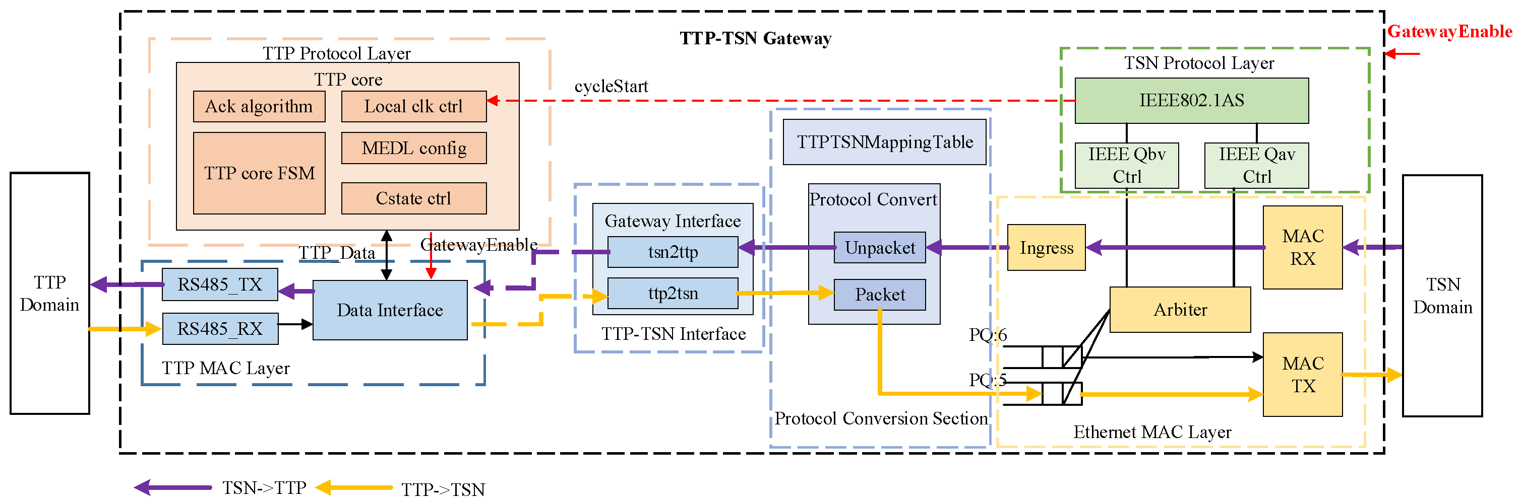
3.3. TTP–TSN Gateway
3.4. TTP–TSN Network Model
3.4.1. Base Model
3.4.2. Low-Latency TTP–TSN Scheduling Model
3.4.3. Model Consistency Analysis
4. Research on Low-Latency TTP–TSN Network Planning
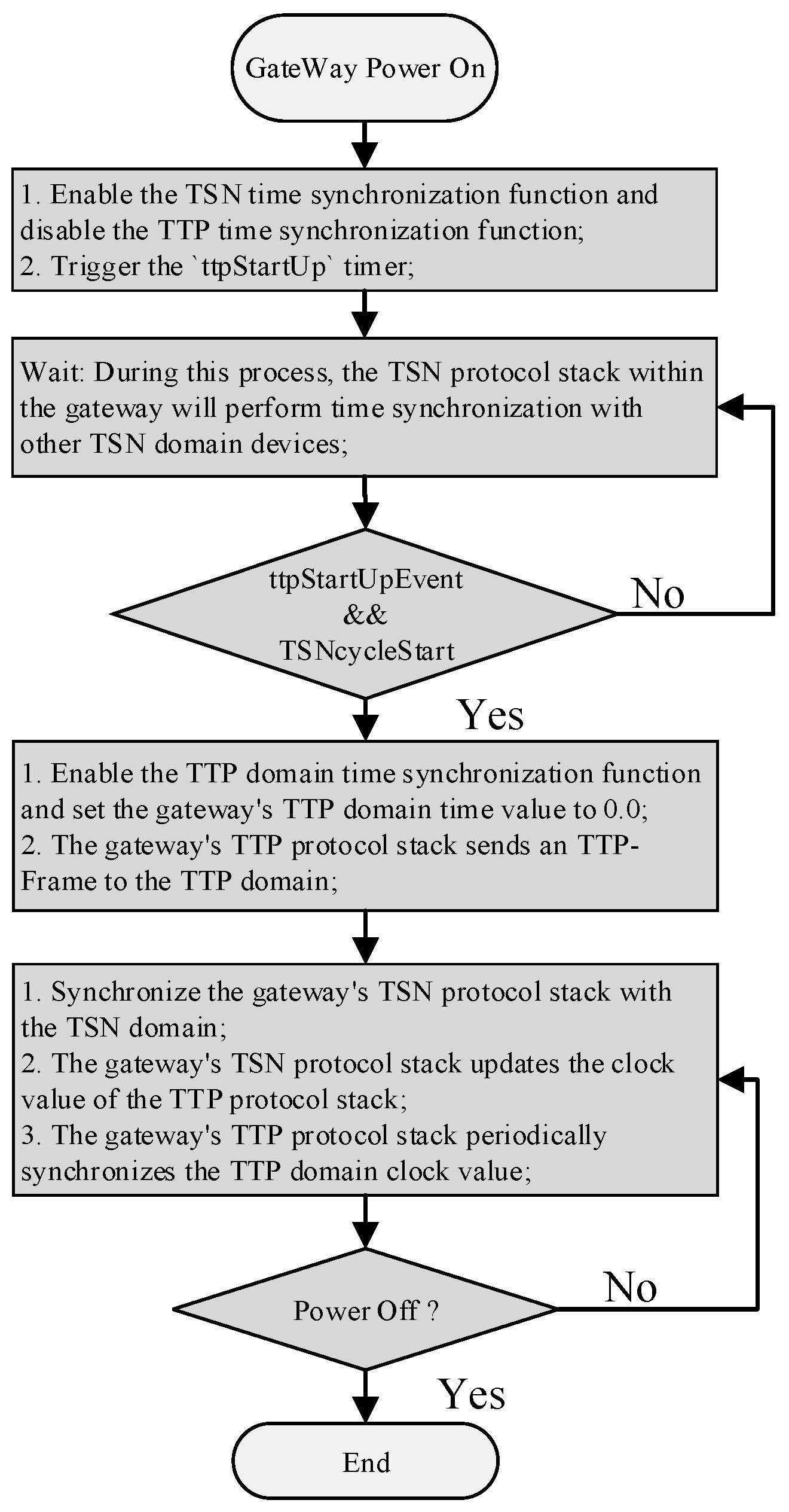
4.1. Engineered Time-Synchronization Algorithm
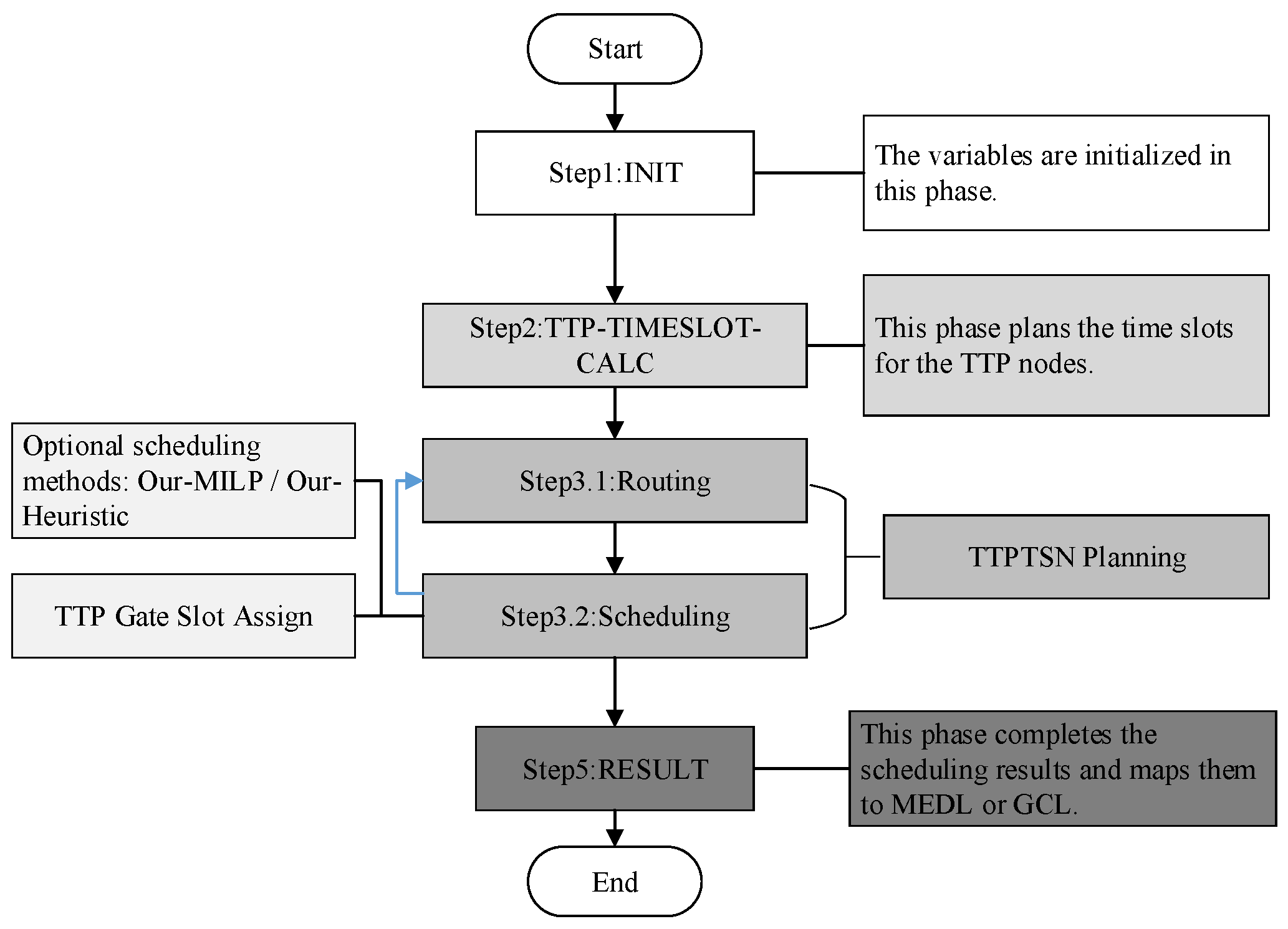
4.2. TTP–TSN Low-Latency Planning Algorithm
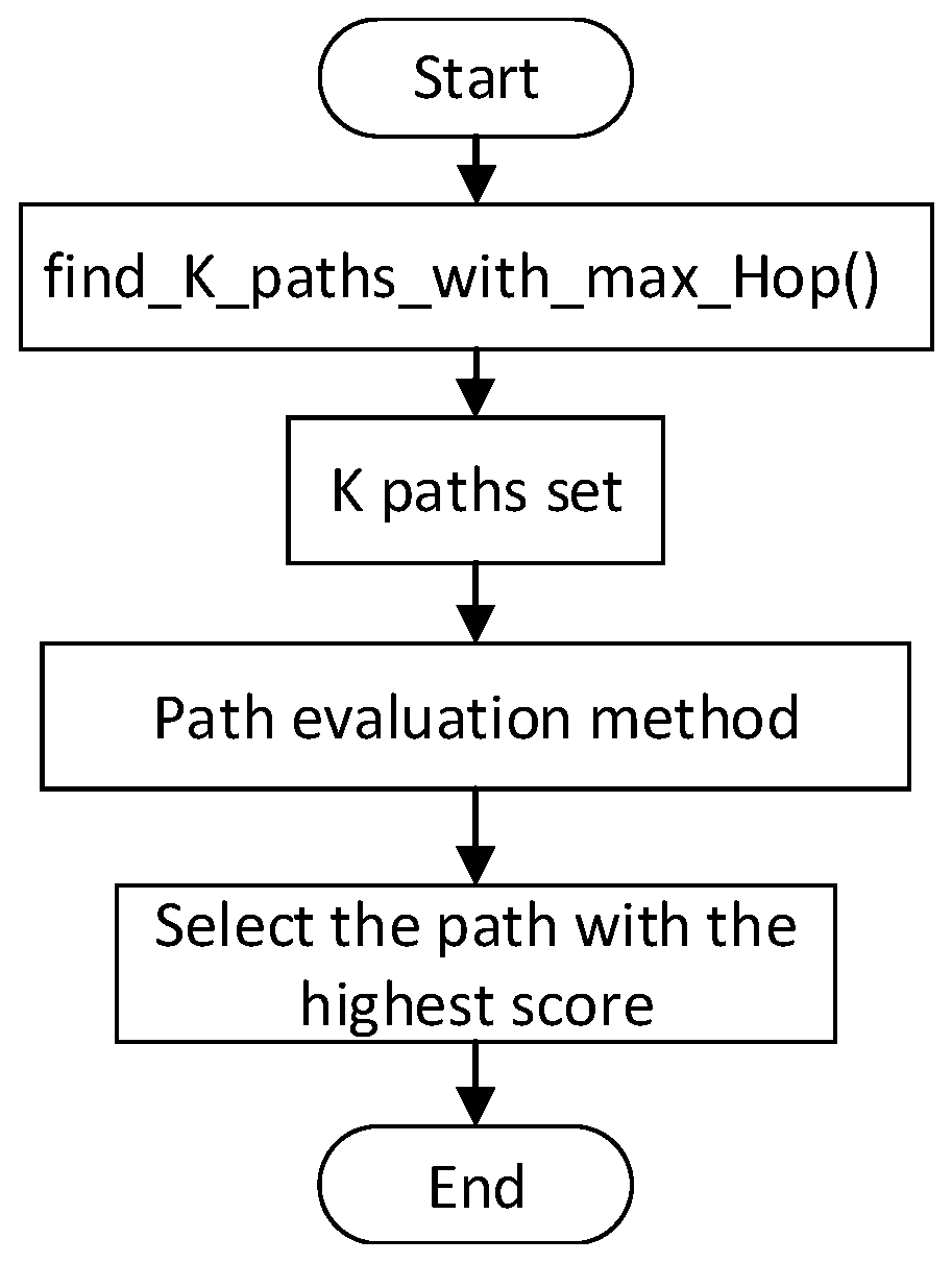
4.2.1. Routing Algorithm
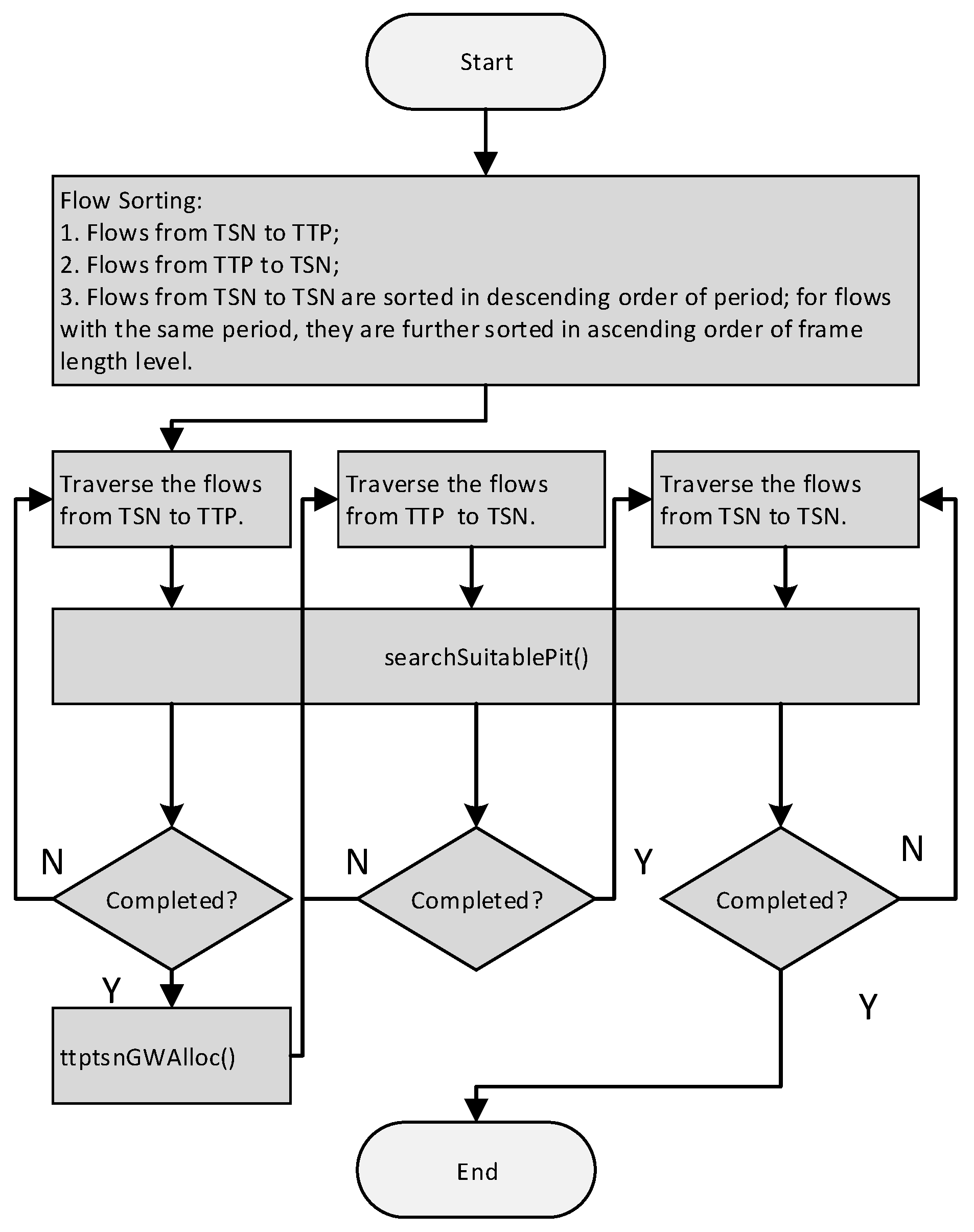
4.2.2. Scheduling Algorithm
| Algorithm 1: searchSuitablePit Algorithm |
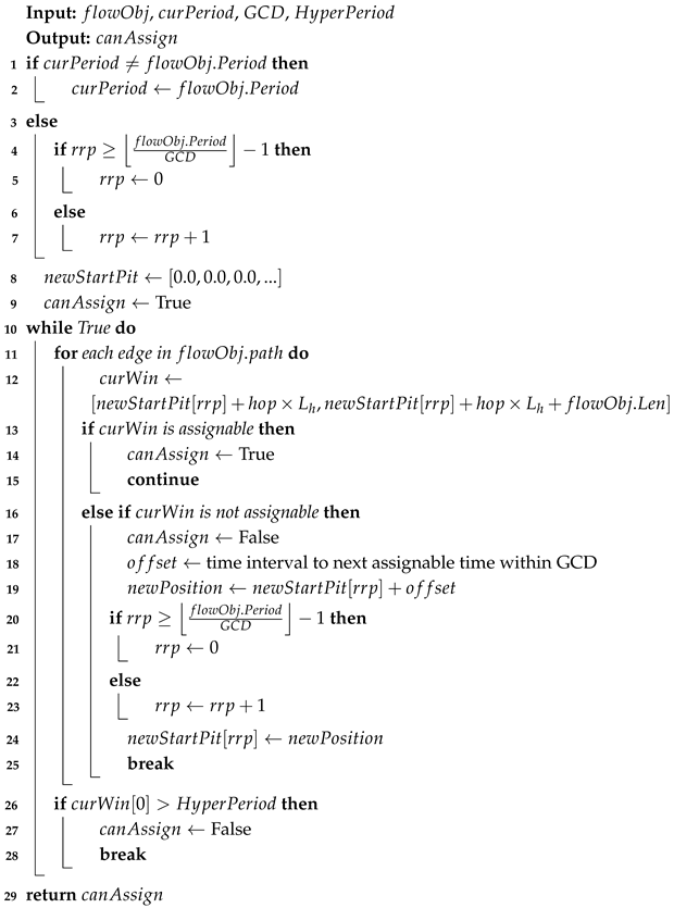 |
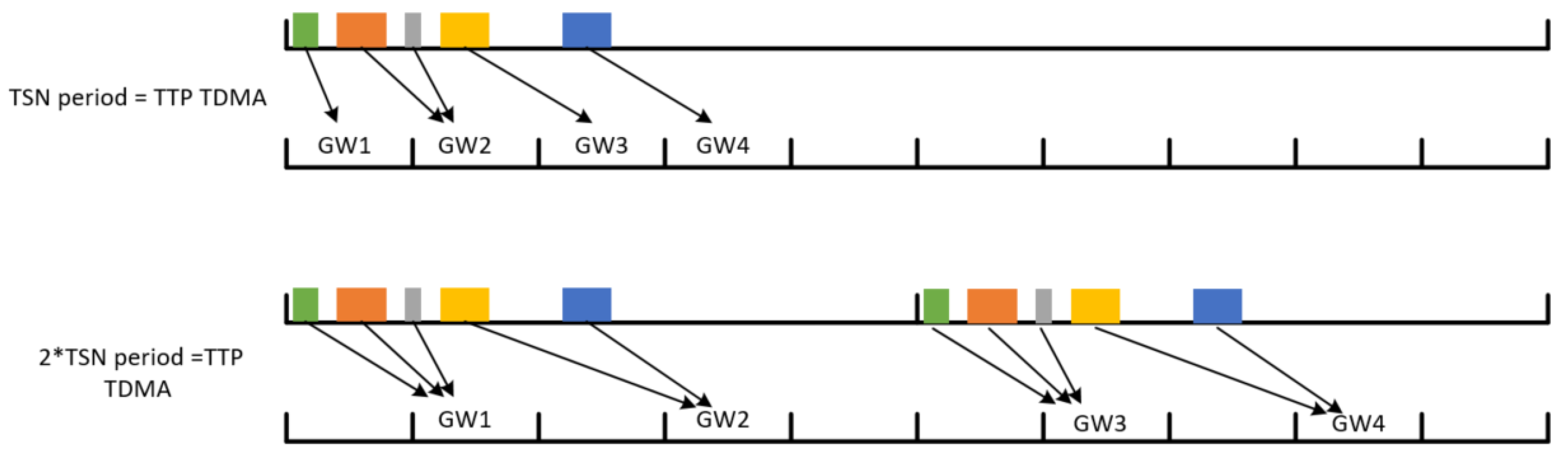
4.2.3. TTP–TSN Gateway-Allocation Method
4.3. Algorithm Analysis
4.3.1. Schedulability Analysis
4.3.2. Approximation Ratio Analysis
4.3.3. Algorithm Complexity Analysis
5. Experiment
5.1. Experimental Environment and Test Stimuli
5.2. Simulation Verification
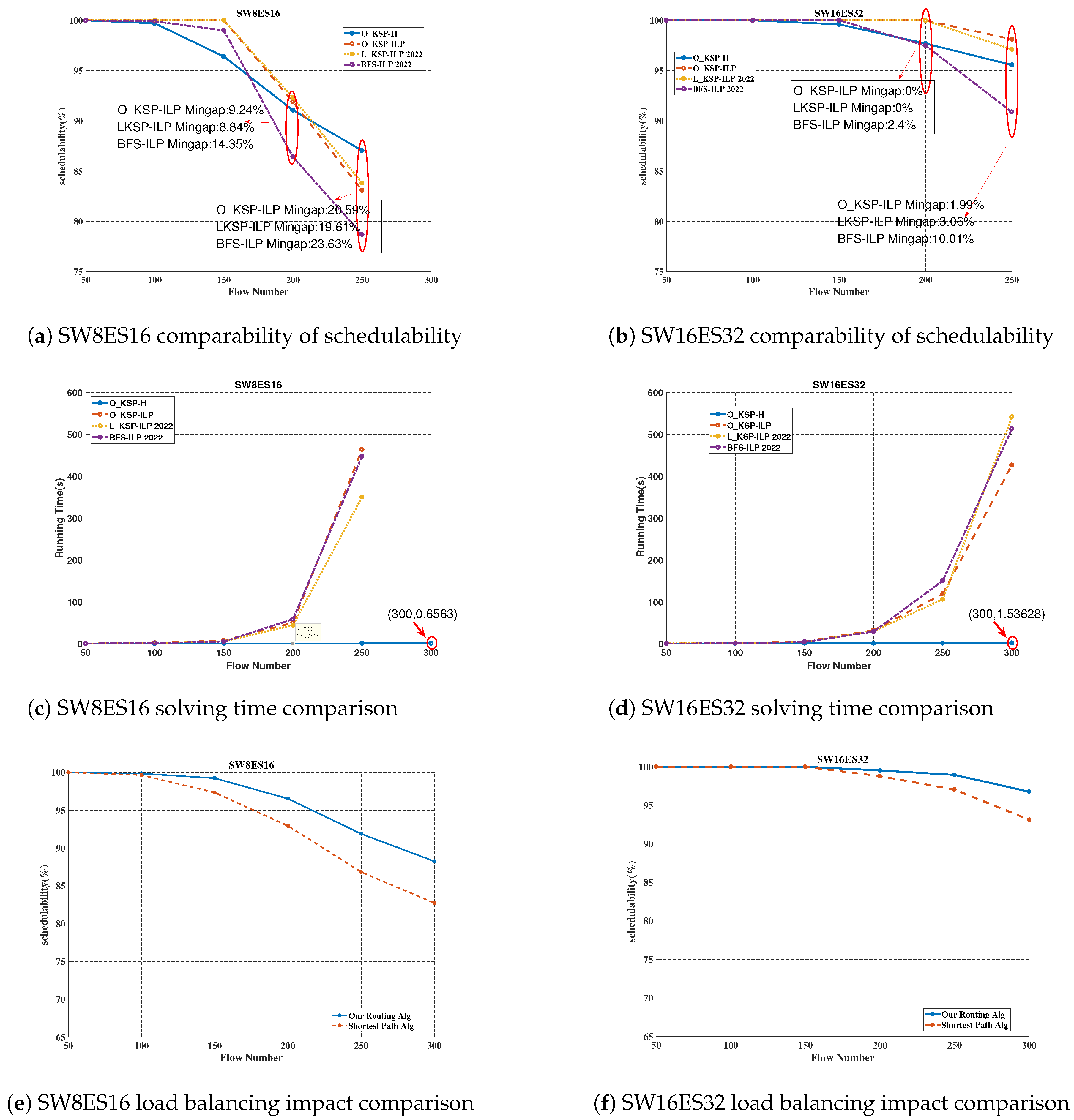
5.2.1. TTP–TSN Routing Verification
5.2.2. TTP–TSN Scheduling Verification
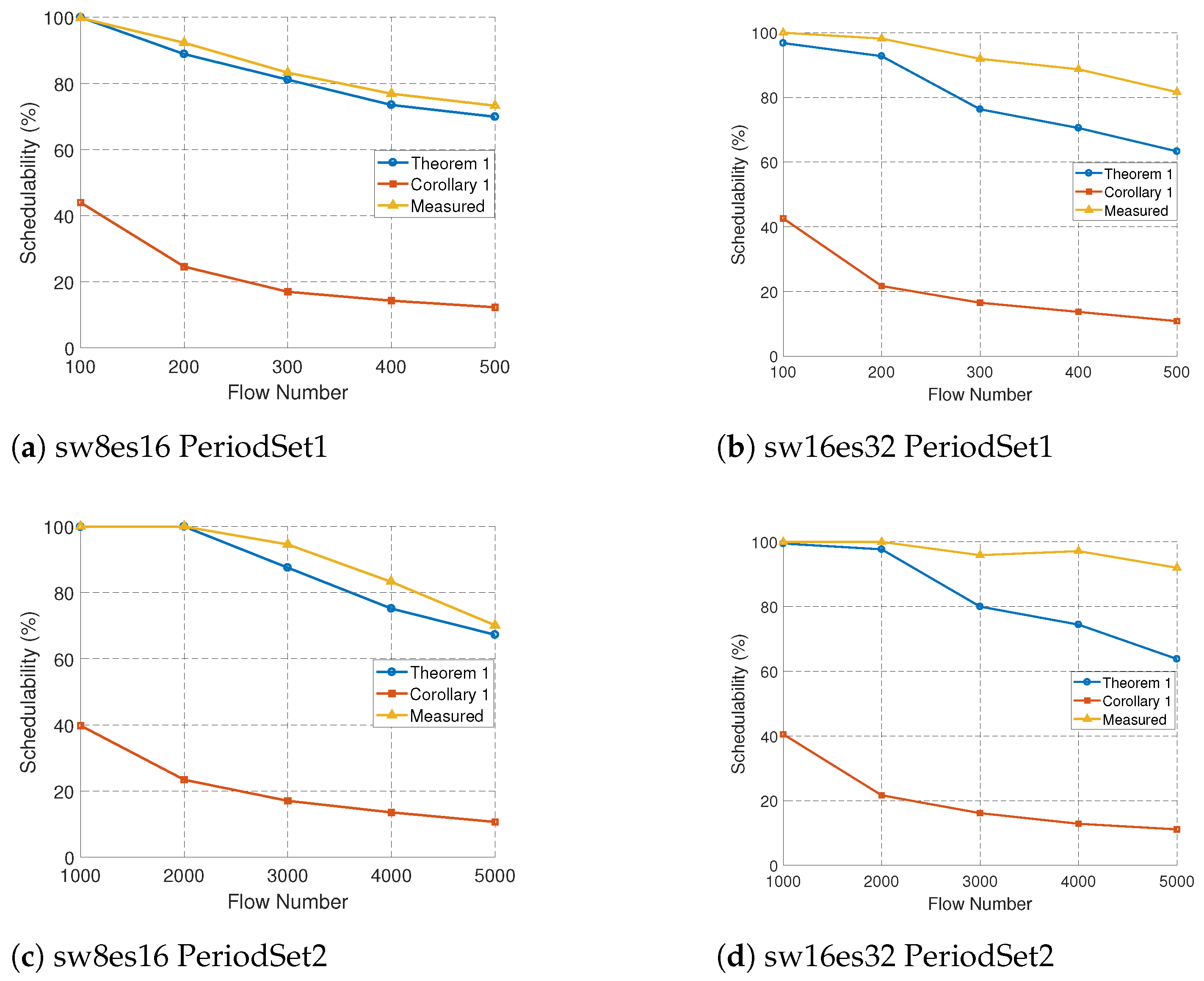
5.2.3. Schedulability Verification
5.2.4. TTP–TSN End-to-End Delay Simulation
5.3. TestBed
5.3.1. Time Synchronization Verification
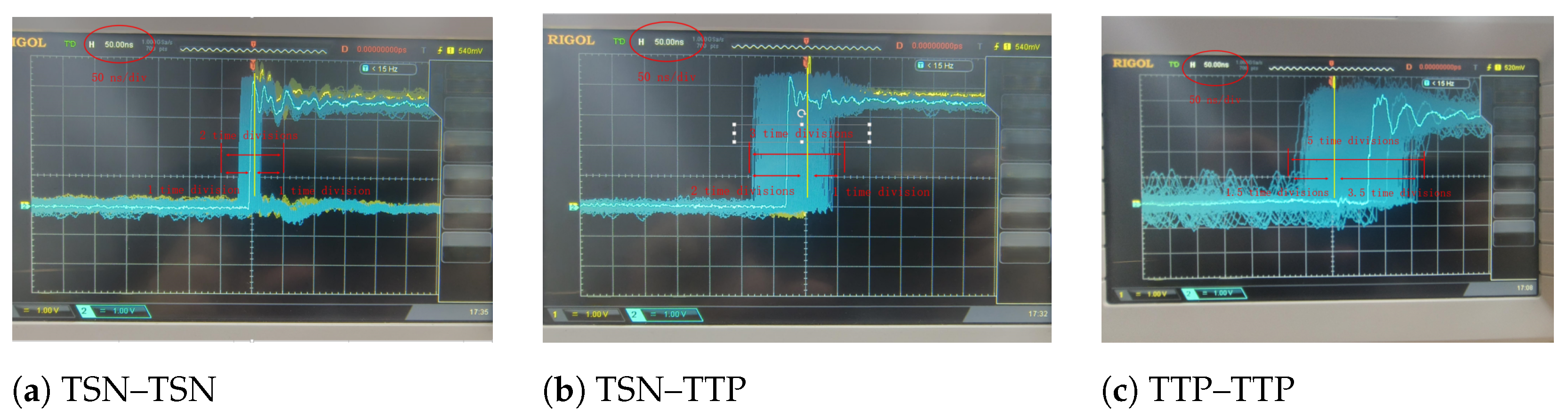
5.3.2. TTP–TSN End-to-End Delay Comparison
6. Conclusions
Author Contributions
Funding
Data Availability Statement
Conflicts of Interest
References
- EE Times Asia. Looking Ahead: High-Speed In-Vehicle Display and Sensor Connections. 2021. Available online: https://www.eetasia.com/looking-ahead-high-speed-in-vehicle-display-and-sensor-connections/ (accessed on 15 December 2024).
- Olumuyiwa, O.; Chen, Y. Virtual CANBUS and Ethernet Switching in Future Smart Cars Using Hybrid Architecture. Electronics 2022, 11, 3428. [Google Scholar] [CrossRef]
- Deredempt, M.-H.; Kollias, V.; Sun, Z.; Canamares, E.; Ricco, P. Spacecraft Data Handling Architecture based on AFDX network. In Proceedings of the Embedded Real Time Software and Systems (ERTS2014), Toulouse, France, 5–7 February 2014. [Google Scholar]
- Rejeb, N.; Mhadhbi, I.; Karim, A.; Salem, A.K.; Ben Saoud, S. AFDX-CAN Architecture for Avionics Applications. Int. J. Comput. Sci. Commun. Inf. Technol. 2014, 1, 7–14. [Google Scholar]
- Center, N.J.S. On Time-Triggered Ethernet in NASA’s Lunar Gateway. In Avionics Architectures Community of Practice; 2020. Available online: https://ntrs.nasa.gov/api/citations/20205005104/downloads/2020-07-26-AA-CoP.pdf (accessed on 15 December 2024).
- Zhou, X.; Xiong, H.; Feng, H. Hybrid partition- and network-level scheduling design for distributed integrated modular avionics systems. Chin. J. Aeronaut. 2020, 33, 308–323. [Google Scholar] [CrossRef]
- Xie, G.; Zhang, Y.; Chen, N.; Chang, W. A High-Flexibility CAN-TSN Gateway with a Low-Congestion TSN-to-CAN Scheduler. IEEE Trans.-Comput.-Aided Des. Integr. Circuits Syst. 2023, 42, 5072–5083. [Google Scholar] [CrossRef]
- Zexiong, L. A Method of Synchronizing the TTE Network with the TTP Bus Network. Patent No. CN108809466A, 13 November 2018. [Google Scholar]
- Albert, A.; Gmbh, R. Comparison of event-triggered and time-triggered concepts with regard to distributed control systems. Embed. World 2004, 2004, 235–252. [Google Scholar]
- Borana, A.; Sonnis, S.; Mohanty, A.; Bhujbal, S.; Roy, D.; Vaidya, U. Design, Simulation and Validation of Fault Tolerant Averaging Algorithm for Clock Synchronization with Custom Time Triggered Deterministic Protocol. IEEE Trans. Ind. Appl. 2022, 58, 5447–5456. [Google Scholar] [CrossRef]
- Zhao, L.; Pop, P.; Steinhorst, S. Quantitative Performance Comparison of Various Traffic Shapers in Time-Sensitive Networking. IEEE Trans. Netw. Serv. Manag. 2022, 19, 2899–2928. [Google Scholar] [CrossRef]
- Herber, C.; Richter, A.; Wild, T.; Herkersdorf, A. Real-time capable CAN to AVB ethernet gateway using frame aggregation and scheduling. In Proceedings of the 2015 Design, Automation & Test in Europe Conference & Exhibition (DATE), Grenoble, France, 9–13 March 2015; pp. 61–66. [Google Scholar] [CrossRef]
- Berisa, A.; Ashjaei, M.; Daneshtalab, M. Investigating and Analyzing CAN-to-TSN Gateway Forwarding Techniques. In Proceedings of the 2023 IEEE 26th International Symposium on Real-Time Distributed Computing (ISORC), Nashville, TN, USA, 23–25 May 2023; pp. 136–145. [Google Scholar] [CrossRef]
- Peng, Y.; Shi, B.; Jiang, T.; Tu, X.; Xu, D.; Hua, K. A Survey on In-Vehicle Time-Sensitive Networking. IEEE Internet Things J. 2023, 10, 14375–14396. [Google Scholar] [CrossRef]
- Chahed, H.; Kassler, A. TSN Network Scheduling—Challenges and Approaches. Network 2023, 3, 585–624. [Google Scholar] [CrossRef]
- Kong, W.; Nabi, M.; Goossens, K. Run-Time Recovery and Failure Analysis of Time-Triggered Traffic in Time Sensitive Networks. IEEE Access 2021, 9, 91710–91722. [Google Scholar] [CrossRef]
- Wang, J.; Zhou, L.; Tian, L. ILP-based multiperiod flow routing and scheduling method in time-sensitive network. J. Phys. Conf. Ser. 2022, 2384, 012032. [Google Scholar] [CrossRef]
- Huang, K.; Wan, X.; Wang, K.; Jiang, X.; Chen, J.; Deng, Q.; Xu, W.; Peng, Y.; Liu, Z. Reliability-Aware Multipath Routing of Time-Triggered Traffic in Time-Sensitive Networks. Electronics 2021, 10, 125. [Google Scholar] [CrossRef]
- Vlk, M.; Hanzálek, Z.; Brejchová, K.; Tang, S.; Bhattacharjee, S.; Fu, S. Enhancing Schedulability and Throughput of Time-Triggered Traffic in IEEE 802.1Qbv Time-Sensitive Networks. IEEE Trans. Commun. 2020, 68, 7023–7038. [Google Scholar] [CrossRef]
- Stüber, T.; Osswald, L.; Lindner, S.; Menth, M. A Survey of Scheduling Algorithms for the Time-Aware Shaper in Time-Sensitive Networking (TSN). IEEE Access 2023, 11, 61192–61233. [Google Scholar] [CrossRef]
- Wang, Z.; Luo, F.; Li, Y.; Gan, H.; Zhu, L. Schedulability Analysis in Time-Sensitive Networking: A Systematic Literature Review. arXiv 2024, arXiv:2407.15031. [Google Scholar]
- Baveja, A.; Srinivasan, A. Approximation Algorithms for Disjoint Paths and Related Routing and Packing Problems. ACM Trans. Algorithms 2000, 25, 255–280. [Google Scholar] [CrossRef]
- Chekuri., C.; Khanna, S. Edge-Disjoint Paths Revisited. ACM Trans. Algorithms 2007, 3, 46. [Google Scholar] [CrossRef]
- Loveless, A. Overview of TTE Applications and Development at NASA/JSC; Technical Report; NASA Johnson Space Center: Houston, TX, USA, 2016. [Google Scholar]
- Dürr, F.; Nayak, N.G. No-wait Packet Scheduling for IEEE Time-sensitive Networks (TSN). In Proceedings of the 24th International Conference on Real-Time Networks and Systems, Brest, France, 19–21 October 2016. [Google Scholar]
- Wang, J.; Liu, C.; Zhou, L.; Wang, J.; Yu, X. DA-DMPF: Delay-aware differential multi-path forwarding of industrial time-triggered flows in deterministic network. Comput. Commun. 2023, 210, 285–293. [Google Scholar] [CrossRef]
- Feng, Z.; Gu, Z.; Yu, H.; Deng, Q.; Niu, L. Online Rerouting and Rescheduling of Time-Triggered Flows for Fault Tolerance in Time-Sensitive Networking. IEEE Trans.-Comput.-Aided Des. Integr. Circuits Syst. 2022, 41, 4253–4264. [Google Scholar] [CrossRef]
- Nie, H.; Li, S.; Liu, Y. An Enhanced Routing and Scheduling Mechanism for Time-Triggered Traffic with Large Period Differences in Time-Sensitive Networking. Appl. Sci. 2022, 12, 4448. [Google Scholar] [CrossRef]
- Korst, J. Periodic Multiprocessor Scheduling; Springer: Berlin/Heidelberg, Germany, 1991. [Google Scholar]


| Symbol | Description |
|---|---|
| Flow object, which contains flow attributes, including Period, Path, and length. | |
| Greatest common divisor of flow periods. | |
| Least common multiple of all flow periods. | |
| Feasibility result. True means the current flow can be successfully assigned to Time Slots; False indicates no slots are available for the current flow. | |
| Round-robin point, indicating the current location on the GCD cycle. | |
| Current active time window. | |
| If the current slot is not valid, the offset gives the adjustment from the starting time. | |
| Switch delay. | |
| P | Flow length level. |
| Flow length interval. | |
| Maximum duration for flow length level P. | |
| Total number of frames in S with period and length level j. | |
| Maximum hop count in the flow set . | |
| Slot length corresponding to flow set . | |
| Probability that m selected flows from flow set have no intersecting paths; this probability can be estimated using the Monte Carlo method. | |
| Probability that m selected flows from flow set have no intersecting paths, but selecting flows results in at least two intersecting paths. | |
| Expected number of flows in the Time Slot with non-intersecting paths. | |
| Maximum duration required by the flow set . | |
| Maximum duration required by the flow set . |
| Experimental Case | Platform | Method Description |
|---|---|---|
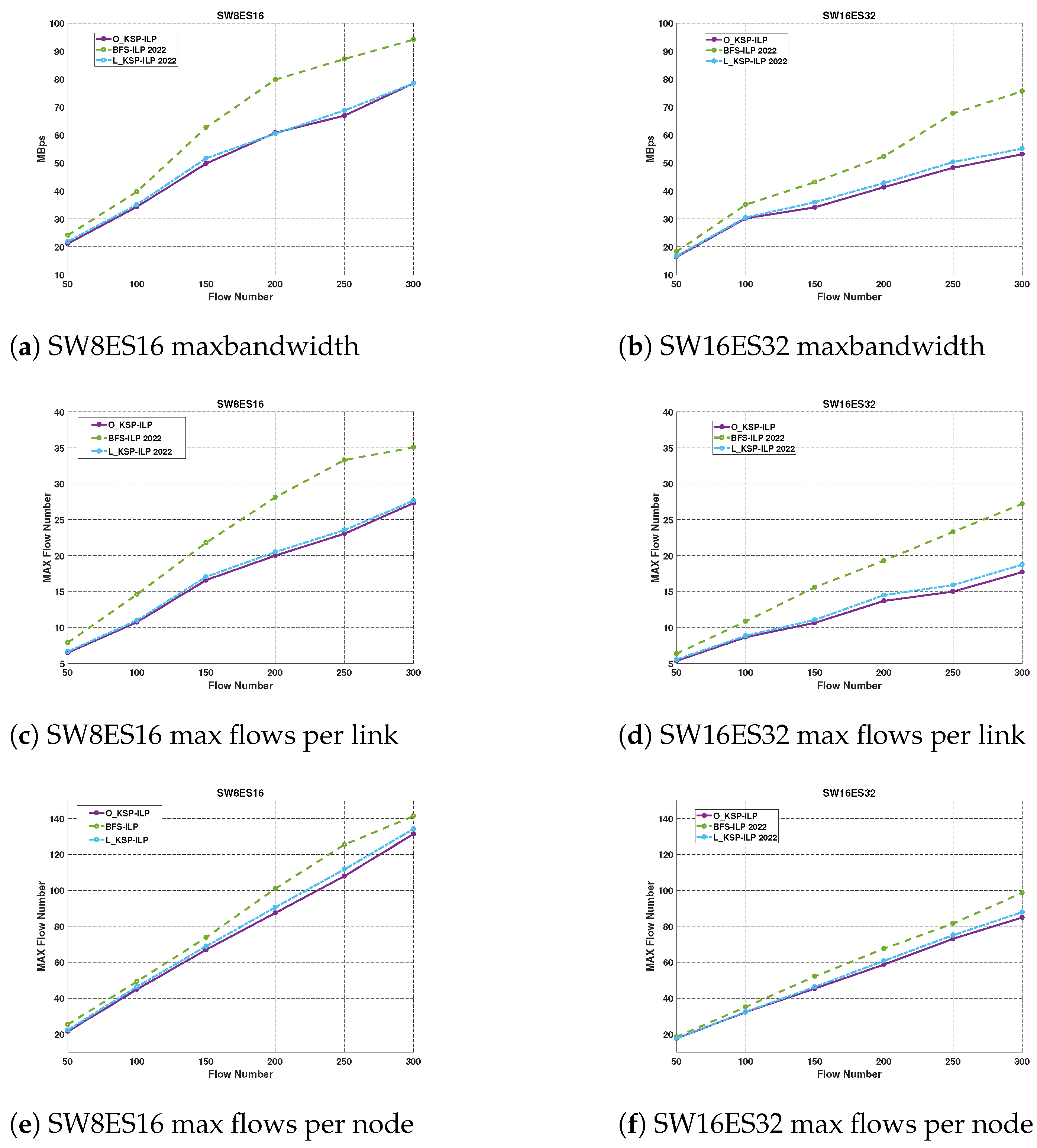
| Planning Algorithm | Python | We compared our algorithm with two others. Firstly, ref. [19] (2022), which used BFS for routing and ILP for scheduling, referred to as ; secondly, ref. [27] (2022), which used a limited KSP algorithm for routing and ILP for scheduling, referred to as . |
| Schedulability Theory | Python | Evaluation of actual scheduling results of Theorem 1, Corollary 1, and the fast algorithm through random experiments. |
| Time Synchronization | FPGA | We used an oscilloscope to verify the time synchronization. |
| End-to-End Delay (comprehensive experiment) | Python and FPGA | We generated 10 flows each for TTP->TSN, TSN->TTP, and TSN->TSN, with flow periods of {1 ms, 2 ms, 4 ms}, and a message length of 20 bytes to simplify the experiment. |
| Parameter | Range |
|---|---|
| Network Scale | {Set1: [8 sw, 16 es], Set2: [16 sw, 32 es]} |
| Flow Period Range | Set1: {100 µs, 200 µs, 400 µs, 500 µs} Set2: {1000 µs, 2000 µs, 4000 µs, 5000 µs} |
| Packet Length Range | {100 bytes, 1500 bytes} |
| ILP Solving Time | 600 s |
| (a) Non-Sched TTP–TSN Communication Delay | |||
| Direction | T = 100 s | T = 200 s | T = 400 s |
| TTP→TSN | 49.928 s | 99.769 s | 199.817 s |
| TSN→TTP | 70.005 s | 140.155 s | 280.097 s |
| Direction | T = 1 ms | T = 2 ms | T = 4 ms |
| TTP→TSN | 500.766 s | 1000.18 s | 1993.69 s |
| TSN→TTP | 699.488 s | 1400.13 s | 2799.85 s |
| (b) Sched TTP–TSN Communication Delay | |||
| Direction | T = 100 s | T = 200 s | T = 400 s |
| TTP→TSN | 0.0 µs | 0.0 µs | 0.0 µs |
| TSN→TTP | 31.599 µs | 71.599 µs | 111.6 µs |
| Direction | T = 1 ms | T = 2 ms | T = 4 ms |
| TTP→TSN | 0.0 s | 0.0 s | 0.0 s |
| TSN→TTP | 301.599 s | 701.599 s | 1101.6 s |
| (a) Non-Sched TTP–TSN Communication Delay | |||
| Direction | T = 1 ms | T = 2 ms | T = 4 ms |
| TTP→TSN | 161.568 µs | 261.288 µs | 461.224 µs |
| TSN→TTP | 765.416 µs | 1465.42 µs | 2865.42 µs |
| (b) Sched TTP–TSN Communication Delay | |||
| Direction | T = 1 ms | T = 2 ms | T = 4 ms |
| TTP→TSN | 67.08 µs | 67.08 µs | 67.08 µs |
| TSN→TTP | 217.92 µs | 413.520 µs | 812.62 µs |
Disclaimer/Publisher’s Note: The statements, opinions and data contained in all publications are solely those of the individual author(s) and contributor(s) and not of MDPI and/or the editor(s). MDPI and/or the editor(s) disclaim responsibility for any injury to people or property resulting from any ideas, methods, instructions or products referred to in the content. |
© 2025 by the authors. Licensee MDPI, Basel, Switzerland. This article is an open access article distributed under the terms and conditions of the Creative Commons Attribution (CC BY) license (https://creativecommons.org/licenses/by/4.0/).
Share and Cite
Peng, Y.; Jiang, T.; Tu, X.; Huang, B.; Guo, Z.; Xu, D. Research on Low-Latency TTP–TSN Cross-Domain Network Planning Problem. Electronics 2025, 14, 203. https://doi.org/10.3390/electronics14010203
Peng Y, Jiang T, Tu X, Huang B, Guo Z, Xu D. Research on Low-Latency TTP–TSN Cross-Domain Network Planning Problem. Electronics. 2025; 14(1):203. https://doi.org/10.3390/electronics14010203
Chicago/Turabian StylePeng, Yifei, Tigang Jiang, Xiaodong Tu, Bolin Huang, Zheng Guo, and Du Xu. 2025. "Research on Low-Latency TTP–TSN Cross-Domain Network Planning Problem" Electronics 14, no. 1: 203. https://doi.org/10.3390/electronics14010203
APA StylePeng, Y., Jiang, T., Tu, X., Huang, B., Guo, Z., & Xu, D. (2025). Research on Low-Latency TTP–TSN Cross-Domain Network Planning Problem. Electronics, 14(1), 203. https://doi.org/10.3390/electronics14010203