GNSS/IMU/ODO Integrated Navigation Method Based on Adaptive Sliding Window Factor Graph

Abstract

One of the predominant technologies for multi-source navigation in vehicles involves the fusion of GNSS/IMU/ODO through a factor graph. To address issues such as the asynchronous sampling frequencies between the IMU and ODO, as well as diminished accuracy during GNSS signal loss, we propose a GNSS/IMU/ODO integrated navigation method based on an adaptive sliding window factor graph. The measurements from the ODO are utilized as observation factors to mitigate prediction interpolation errors associated with traditional ODO pre-integration methods. Additionally, online estimation and compensation for both installation angle deviations and scale factors of the ODO further enhance its ability to constrain pose errors during GNSS signal loss. A multi-state marginalization algorithm is proposed and then utilized to adaptively adjust the sliding window size based on the quality of GNSS observations, enhancing pose optimization accuracy in multi-source fusion while prioritizing computational efficiency. Tests conducted in typical urban environments and mountainous regions demonstrate that our proposed method significantly enhances fusion navigation accuracy under complex GNSS conditions. In a complex city environment, our method achieves a 55.3% and 29.8% improvement in position and velocity accuracy and enhancements of 32.0% and 61.6% in pitch and heading angle accuracy, respectively. These results match the precision of long sliding windows, with a 75.8% gain in computational efficiency. In mountainous regions, our method enhances the position accuracy in the three dimensions by factors of 89.5%, 83.7%, and 43.4%, the velocity accuracy in the three dimensions by factors of 65.4%, 32.6%, and 53.1%, and reduces the attitude errors in roll, pitch, and yaw by 70.5%, 60.8%, and 26.0%, respectively, demonstrating strong engineering applicability through an optimal balance of precision and efficiency.

1. Introduction

In recent years, the rapid development of intelligent driving technology and the automotive industry has driven a growing demand for high-precision vehicle navigation and positioning [1]. In complex urban environments, navigation systems relying on a single sensor are insufficient to meet the high standards of accuracy and reliability required. As a result, multi-sensor fusion navigation has become an inevitable trend in this field’s development. The Global Navigation Satellite System (GNSS), Inertial Measurement Unit (IMU), and wheel Odometers (ODOs) are currently the most commonly used sensors for vehicle navigation. Their ease of installation and accessibility make the GNSS/INS/ODO fusion scheme one of today’s mainstream approaches. By leveraging the complementary strengths of each sensor, this method achieves high-performance navigation and positioning results [2].

Currently, multi-sensor information fusion algorithms primarily encompass the Kalman filter and factor graph methodologies. The Kalman filter has been extensively developed and is widely applied in navigation and positioning domains [3,4]. In recent years, factor graphs have emerged as a nonlinear optimization technique frequently utilized in the field of robotics [5], particularly for applications involving vision, LiDAR, and simultaneous localization and mapping (SLAM) [6]. This approach demonstrates superior performance and robustness compared to Kalman filter fusion when integrating diverse classes of heterogeneous sensors seamlessly [7]. Additionally, GNSS/INS information fusion has exhibited significant application potential and is increasingly becoming a focal point of research [8,9]. Li et al. employed factor graphs for tight coupling, achieving superior performance compared to the Kalman filter [10]. Integrating ODO information during GNSS out-of-lock periods can effectively mitigate inertial navigation divergence [11]. The ODO is integrated as a pre-integration component within the factor graph optimization framework [12]. However, the sampling frequencies of both IMU and ODO are often unsynchronized, necessitating interpolation of ODO predictions. Predictive interpolation is generally unsuitable for highly dynamic motion scenarios and functions primarily as a post-processing method, lacking real-time application potential [13].

In complex urban environments, the quality of GNSS observations is significantly compromised by external factors, such as multipath effect [14], NLOS signals [15] and shade [16]. However, most existing GNSS/INS fusion schemes optimized through factor graphs utilize fixed-length sliding windows [17], which fail to effectively adapt to the dynamic and variable conditions of GNSS signals. Utilizing a shorter observation window may hinder the full exploitation of effective GNSS data, consequently impeding the attainment of high positioning accuracy, while a longer window can lead to diminished computational efficiency and unnecessary consumption of resources. To address this issue, this paper proposes an information fusion scheme that adaptively adjusts the length of the sliding window based on the quality of GNSS observations within it, balancing both fusion optimization performance and computational efficiency. By leveraging real-time measurements from wheel odometers as observation factors, the scale factor and installation deviation angle of these devices are estimated to further enhance positioning performance.

This paper outlines the basic framework of factor graph optimization and details the algorithm and process of adaptive sliding window factor graph fusion. The feasibility of using ODO measurements as a factor is validated and the effectiveness of the adaptive sliding window approach is demonstrated through real-world vehicle tests. Finally, we analyze and discuss the potential applications and future prospects of the improved method.

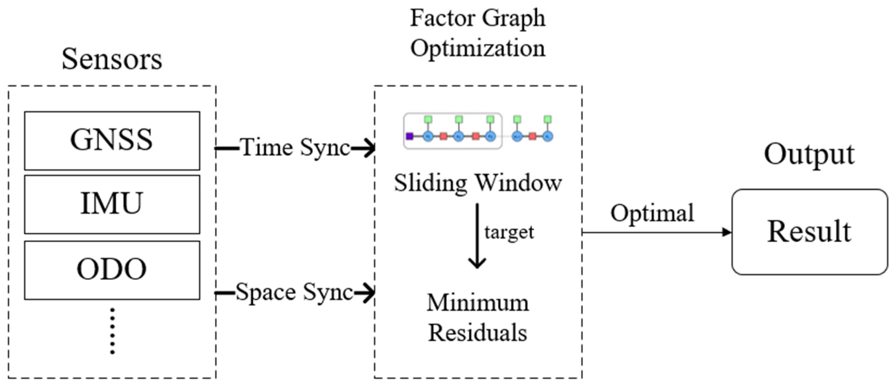
2. Fusion Framework Based on Factor Graph

Due to the susceptibility of GNSS to environmental factors that diminish positioning accuracy, the GNSS/IMU/ODO fusion algorithm based on the factor graph is constantly improved and optimized. Jiang et al. incorporated the effects of Earth’s rotation into the pre-integration factor, further enhancing fusion accuracy [18]. On this basis, Tang et al. summarized the basic principle of factor graphs [19]. The basic framework of the fusion navigation algorithm based on a factor graph is shown in Figure 1, where each sensor is treated as a factor for fusion and optimized within a window [20]. Measurement data from multi-source sensors such as GNSS, IMU, and ODO are synchronized in both time and space before being fused using a factor graph approach. When the residual error within the sliding window is minimized to an optimal level, the final navigation result is output.

Figure 2 illustrates the schematic diagram of the factor graph sliding window optimization algorithm, which processes IMU/ODO joint pre-integration along with GNSS position information.

Here, ${\mathit{x}}_t$ represents the state variables at a time $t$, meaning the following:

$${\mathit{x}}_t={\left[{\left({\mathit{p}}_{w{b}_t}^w\right)}^{\mathrm{T}},{\left({\mathit{q}}_{w{b}_t}^w\right)}^{\mathrm{T}},{\left({\mathit{v}}_{w{b}_t}^w\right)}^{\mathrm{T}},{\left({\mathit{b}}_{g_t}\right)}^{\mathrm{T}},{\left({\mathit{b}}_{a_t}\right)}^{\mathrm{T}},{\left({\mathit{s}}_t^{t-1}\right)}^{\mathrm{T}},{\left(sod{o}_t\right)}^{\mathrm{T}}\right]}^{{\mathrm{T}}_a}$$

(1)

where “w-frame” denotes the world coordinate system, which is equivalent to the navigation coordinate system “n-frame” at the initial moment, ${\mathit{p}}_{w{b}_t}^w$ represents the position of the carrier at a time $t$ in w-frame, ${\mathit{q}}_{w{b}_t}^w$ denotes the attitude quaternion, ${\mathit{v}}_{w{b}_t}^w$ represents the velocity, ${\mathit{b}}_{g_t}$ and ${\mathit{b}}_{a_t}$ indicate the gyro and accelerometer biases, respectively. ${\mathit{s}}_t^{t-1}$ stands for the distance traveled from time $t-1$ to $t$, and $sod{o}_t$ represents the wheel odometer scale factor. T means matrix transpose. ${\mathrm{T}}_a$ means transposing all elements.

All the states within the sliding window, as shown in Figure 2, are optimized using a factor graph with the optimization criteria defined in Equation (2).

$${\mathit{X}}^{MAP}=\arg \min \left\{\begin{array}{l}{\Vert {\mathbf{r}}_p-{\mathbf{H}}_p\mathit{X}\Vert }^2+{\displaystyle \sum _{k\in [1,n]}{\Vert {\mathbf{r}}_{IMU/ODO}^{\mathrm{Pr}e}({\widehat{z}}_{k-1,k}^{\mathrm{Pr}e},\mathit{X})\Vert }_{{\sum }_{k-1,k}^{\mathrm{Pr}e}}^2}\\ +{\displaystyle \sum _{i\in [0,m]}{\Vert {\mathbf{r}}_{GNSS}({\widehat{z}}_i^{GNSS},\mathit{X})\Vert }_{{\sum }_i^{GNSS}}^2}\end{array}\right\}$$

(2)

where $\mathit{X}$ represents the states to be optimized within the sliding window, ${\Vert •\Vert }_{{\sum }_j}^2$ denotes the Mahalanobis distance [21], ${\mathbf{r}}_p-{\mathbf{H}}_p\mathit{X}$ is the prior factor residual term, ${\mathbf{r}}_{IMU/ODO}^{\mathrm{Pr}e}({\widehat{\mathit{z}}}_{k-1,k}^{\mathrm{Pr}e},\mathit{X})$ represents the IMU/ODO joint pre-integration factor residual term between two adjacent states $t_{k-1}$ and $t_k$, and ${\mathbf{r}}_{GNSS}({\widehat{z}}_i^{GNSS},\mathit{X})$ is the GNSS factor residual term at a time $t_i$. By solving this nonlinear least-squares problem using the Gauss–Newton method, the optimal solution for all states in the window can be obtained [22]. The Ceres Solver library is employed to solve the optimization problem [23].

The existing factor graph fusion scheme, based on IMU/ODO combined pre-integration and a fixed sliding window, presents the following challenges:

• Inconsistent Sampling Frequencies: In the current approach, the wheel odometer is incorporated through pre-integration, requiring consistent sampling frequencies between the inertial navigation system and the wheel odometer. However, in practical engineering, the wheel odometer’s sampling frequency is often lower than that of the inertial navigation system. Interpolating wheel odometer data is the typical solution, but in highly dynamic scenarios, interpolation introduces errors and relies on future measurements, limiting its potential for real-time applications;
• Spatial Synchronization Issues: Factor graph optimization requires spatial synchronization. While the IMU’s translation parameters can be derived from the vehicle’s structural dimensions, accurately measuring the installation angle is difficult. Misalignment between the IMU and ODO reference frames can degrade fusion performance;
• Limitations of Fixed-Length Sliding Windows: Most fusion schemes use fixed-length sliding windows, which struggle to adapt to varying GNSS signal conditions. Short windows fail to fully utilize effective GNSS observations for high-precision positioning, while longer windows reduce computational efficiency and waste resources.

To address these issues, we propose a fusion algorithm that incorporates the wheel odometer as a factor, eliminating the frequency mismatch with the IMU. The method estimates the installation angle as a state parameter, synchronizes sensor spatial data, improves positioning and attitude accuracy, and implements an adaptive sliding window scheme that adjusts window size based on GNSS quality, balancing both accuracy and efficiency.

3. ODO Factor Algorithm

To address the challenges posed by high dynamic scenarios and the real-time applicability issues of ODO interpolation in existing factor graphs, this study directly incorporates wheel odometer measurement data into the factor graph optimization as a direct measurement factor. This approach enhances practical applicability. The fusion diagram is depicted in Figure 3, where ODO is used as an observational factor rather than as a pre-integral.

In accordance with the principles of factor graph optimization, the ODO acquires measurement data pertaining to forward velocity. It is necessary to construct the residual difference between the measured and calculated speed values, along with the corresponding Jacobian matrix.

Assuming that the output of ODO at a time $t$ is ${\mathit{v}}_t^o={\left[\begin{array}{ccc}{\tilde{v}}^i(1+sodo)& 0& 0\end{array}\right]}^{\mathrm{T}}$, where the o-frame represents the coordinate system of ODO, the relationship for speed conversion between IMU and ODO is shown in Equation (3).

$${\widehat{\mathit{v}}}_{m{o}_t}^m={\widehat{\mathit{v}}}_{m{b}_t}^m+{\mathit{C}}_{b_t}^m\left[{\mathit{\omega }}_{m{b}_t}^{b_t}\times \right]{\mathit{l}}_{odo}^b$$

(3)

where the m-frame is the carrier coordinate system b-frame at the initial time, the attitude rotation matrix of the carrier under the m-frame at a time $t$ is ${\mathit{C}}_{b_t}^m$, ${\mathit{\omega }}_{m{b}_t}^{b_t}$ is the angular velocity at a time $t$, ${\mathit{l}}_{odo}^b$ is the lever arm of the IMU and ODO, and ${\widehat{\mathit{v}}}_{m{o}_t}^m$ and ${\widehat{\mathit{v}}}_{m{b}_t}^m$ represents the velocity of ODO and IMU under the m-frame.

Convert the wheel odometer measurements to the m-frame system,

$${\tilde{\mathit{v}}}_{m{o}_t}^m={\mathit{C}}_b^m{\mathit{C}}_o^b{\mathit{v}}_t^o$$

(4)

where ${\mathit{v}}_t^o$ is the output velocity of the ODO, and ${\mathit{C}}_o^b$ and ${\mathit{C}}_b^m$ are the rotation matrix of the corresponding coordinate system transformation of the respective angle markers. By subtracting Equations (3) and (4), the residual between the measured and calculated values of the wheel odometer can be obtained.

$${\widehat{\mathit{v}}}_{m{o}_t}^m-{\tilde{\mathit{v}}}_{m{o}_t}^m={\widehat{\mathit{v}}}_{m{b}_t}^m+{\mathit{C}}_{b_t}^m\left[{\mathit{\omega }}_{m{b}_t}^{b_t}\times \right]{\mathit{l}}_{odo}^b-{\mathit{C}}_b^m{\mathit{C}}_o^b{\mathit{v}}_t^o$$

(5)

Since all state variables solved through factor graph optimization are in the w-frame, directly combining wheel speedometer observations with the state variables in Equation (5) complicates the derivation process. Therefore, the residual vector of the ODO factor is obtained by transforming Equations (5) and (6).

$${\mathit{r}}_{odo}\left({\mathit{z}}_i^{odo},\mathit{X}\right)={\mathit{C}}_w^{b_t}{\widehat{\mathit{v}}}_{w{b}_t}^w+\left[{\mathit{\omega }}_{m{b}_t}^{b_t}\times \right]{\mathit{l}}_{odo}^b-{\widehat{\mathit{C}}}_o^b{\tilde{\mathit{v}}}^o$$

(6)

where ${\widehat{\mathit{C}}}_o^b$ is the identity matrix without considering the installation angle.

By using ODO as a measurement factor, the mileage term is omitted from the state variables shown in Equation (1).

$${\mathit{x}}_t={\left[{\left({\mathit{p}}_{w{b}_t}^w\right)}^{\mathrm{T}},{\left({\mathit{q}}_{w{b}_t}^w\right)}^{\mathrm{T}},{\left({\mathit{v}}_{w{b}_t}^w\right)}^{\mathrm{T}},{\left({\mathit{b}}_{g_t}\right)}^{\mathrm{T}},{\left({\mathit{b}}_{a_t}\right)}^{\mathrm{T}},{\left(sod{o}_t\right)}^{\mathrm{T}}\right]}^{\mathrm{T}}$$

(7)

Equation (6) takes the derivative of each state variable shown in Equation (7) to obtain the Jacobian matrix of residual ${\mathit{r}}_{odo}\left({\mathit{z}}_i^{odo},\mathit{X}\right)$ relative to $\mathit{X}$.

$${\displaystyle \frac{\partial {\mathit{r}}_{odo}\left({\mathit{z}}_i^{odo},\mathit{X}\right)}{\partial \mathit{X}}}=\left[\begin{array}{cccccc}{\mathbf{0}}_{3\times 3}& \left[{\widehat{\mathit{C}}}_w^b{\widehat{\mathit{v}}}_{w{b}_t}^w\times \right]& {\mathit{C}}_w^{b_t}& {\mathit{l}}_{odo}^b\times & {\mathbf{0}}_{3\times 3}& {\displaystyle \frac{\partial }{\partial sodo}}{\left[-{\tilde{\mathit{v}}}^v\right]}_x\end{array}\right]$$

(8)

where ${\mathbf{0}}_{3\times 3}$ means a 3 times 3 zero matrix and ${[•]}_x$ means take the first row of the matrix.

Therefore, the ODO, as a factor, is added to the factor graph fusion scheme, and the problem can be solved by the Ceres Solver.

4. Estimation of ODO Scale Factor and Installation Angle

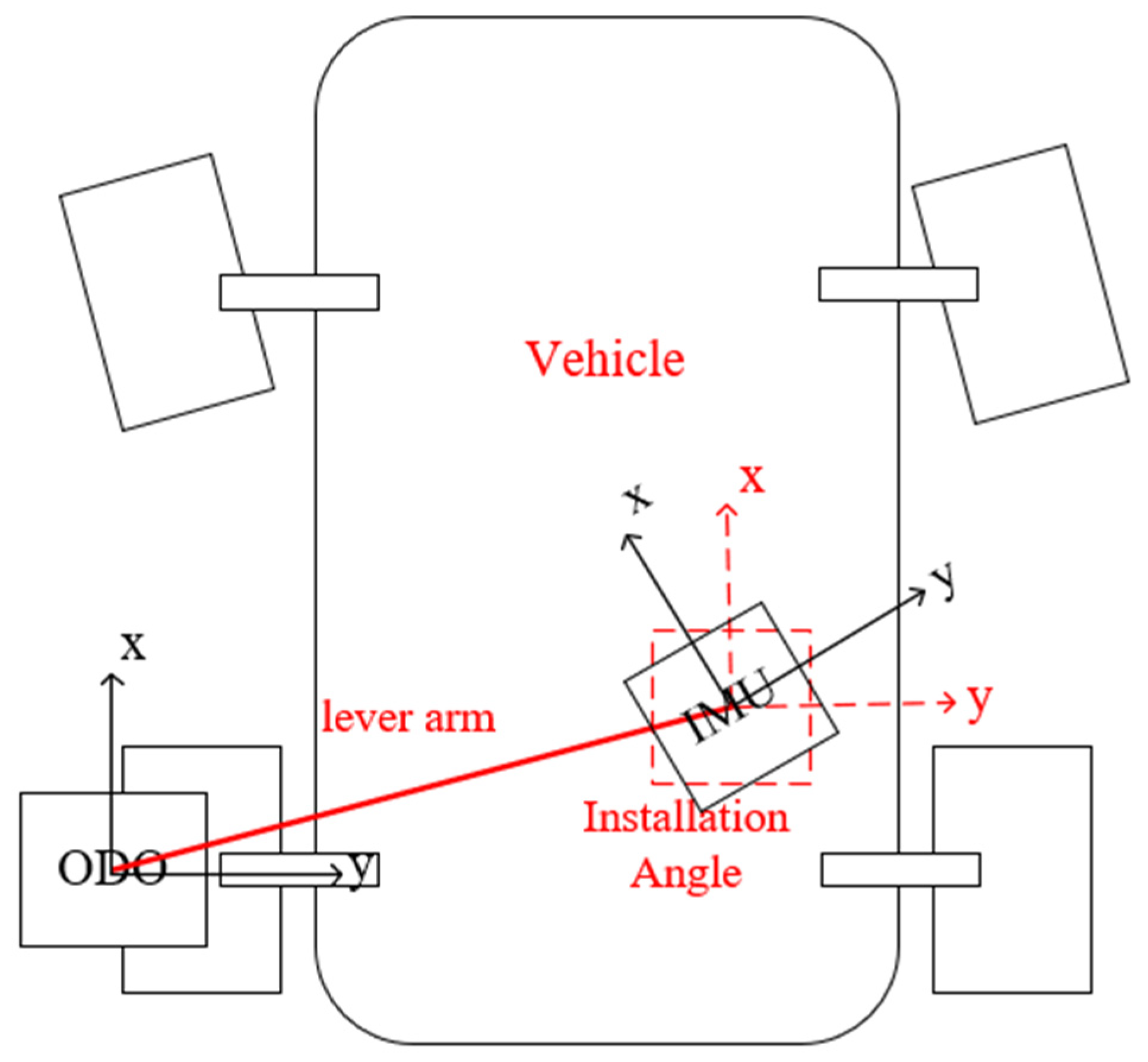
In practical engineering applications, using the wheel odometer for assistance requires accurately determining the lever arm and installation angle to establish the conversion relationship between the carrier coordinate system and the inertial navigation coordinate system, ensuring spatial synchronization for the fusion algorithm. Figure 4 is a schematic diagram of the lever arm and the installation angle. In the figure, the line between ODO and IMU represents the lever arm, and the difference between IMU realization and dashed line represents the installation angle.

The lever arm can be measured from the installation structure with minimal error, but the installation angle is more difficult to measure, so it is added to the state variables for estimation. Literature [24] proposes an external parameter estimation method based on IMU/ODO pre-integration. However, since the installation angle is estimated within the pre-integration factor, the residual variables involved are complex, making the calculation of the Jacobian matrix and the state update process more cumbersome. In contrast, using the ODO as a factor for estimating the installation angle only involves the ODO factor and the state variables without affecting the residuals in other factors. This method is simpler and more straightforward in both principle and application.

Add the installation angle variable to Equation (7).

$${\mathit{x}}_t={\left[{\left({\mathit{p}}_{w{b}_t}^w\right)}^{\mathrm{T}},{\left({\mathit{q}}_{w{b}_t}^w\right)}^{\mathrm{T}},{\left({\mathit{v}}_{w{b}_t}^w\right)}^{\mathrm{T}},{\left({\mathit{b}}_{g_t}\right)}^{\mathrm{T}},{\left({\mathit{b}}_{a_t}\right)}^{\mathrm{T}},{\left(sod{o}_t\right)}^{\mathrm{T}},{(\mathit{a}\mathit{b}\mathit{o})}^{\mathrm{T}}\right]}^{\mathrm{T}}$$

(9)

where $\mathit{a}\mathit{b}\mathit{o}$ represents the angle of the b-frame and o-frame. In theory, the installation angle of the carrier is represented as a three-dimensional vector that includes the roll angle (ϕ), pitch angle (θ), and heading angle (ψ). The rotation matrix for each angle can be expressed as follows:

$${\mathit{C}}_{\varphi }=\left[\begin{array}{ccc}1& 0& 0\\ 0& \cos \varphi & \sin \varphi \\ 0& -\sin \varphi & \cos \varphi \end{array}\right],{\mathit{C}}_{\theta }=\left[\begin{array}{ccc}\cos \theta & 0& -\sin \theta \\ 0& 1& 0\\ \sin \theta & 0& \cos \theta \end{array}\right],{\mathit{C}}_{\psi }=\left[\begin{array}{ccc}\cos \psi & \sin \psi & 0\\ -\sin \psi & \cos \psi & 0\\ 0& 0& 1\end{array}\right]$$

(10)

Since the ODO measures forward speed ${\mathit{v}}_t^o={\left[\begin{array}{ccc}{\tilde{v}}^i(1+sodo)& 0& 0\end{array}\right]}^T$, multiplying it by the left matrix ${\mathit{C}}_{\varphi }$ does not yield any effect; in other words, the roll angle cannot be estimated using this method, so $\mathit{a}\mathit{b}\mathit{o}={\left[\theta ,\psi \right]}^T$.

After incorporating the installation angle error, ${\mathit{C}}_o^b$ in Equation (6) must be determined based on the installation angle. The residual vector of the ODO factor and the Jacobian matrix are presented in Equations (11) and (12), respectively.

$${\mathit{r}}_{odo}\left({\mathit{z}}_i^{odo},\mathit{X}\right)={\mathit{C}}_w^{b_t}{\widehat{\mathit{v}}}_{w{b}_t}^w+\left[{\mathit{\omega }}_{m{b}_t}^{b_t}\times \right]{\mathit{l}}_{odo}^b-{\tilde{\mathit{C}}}_o^b{\tilde{\mathit{v}}}^o$$

(11)

$${\displaystyle \frac{\partial {\mathit{r}}_{odo}\left({\mathit{z}}_i^{odo},\mathit{X}\right)}{\partial \mathit{X}}}=\left[\begin{array}{ccccccc}{\mathbf{0}}_{3\times 3}& \left[{\widehat{\mathit{C}}}_w^b{\widehat{\mathit{v}}}_{w{b}_t}^w\times \right]& {\mathit{C}}_w^{b_t}& {\mathit{l}}_{odo}^b\times & {\mathbf{0}}_{3\times 3}& {\displaystyle \frac{\partial }{\partial sodo}}{\left[-{\mathit{C}}_o^b{\tilde{\mathit{v}}}^o\right]}_x& {\mathit{C}}_o^b{\left[{\tilde{\mathit{v}}}^o\times \right]}_{2,3}\end{array}\right]$$

(12)

where ${[•]}_{2,3}$ means take the 2nd and 3rd columns of the matrix.

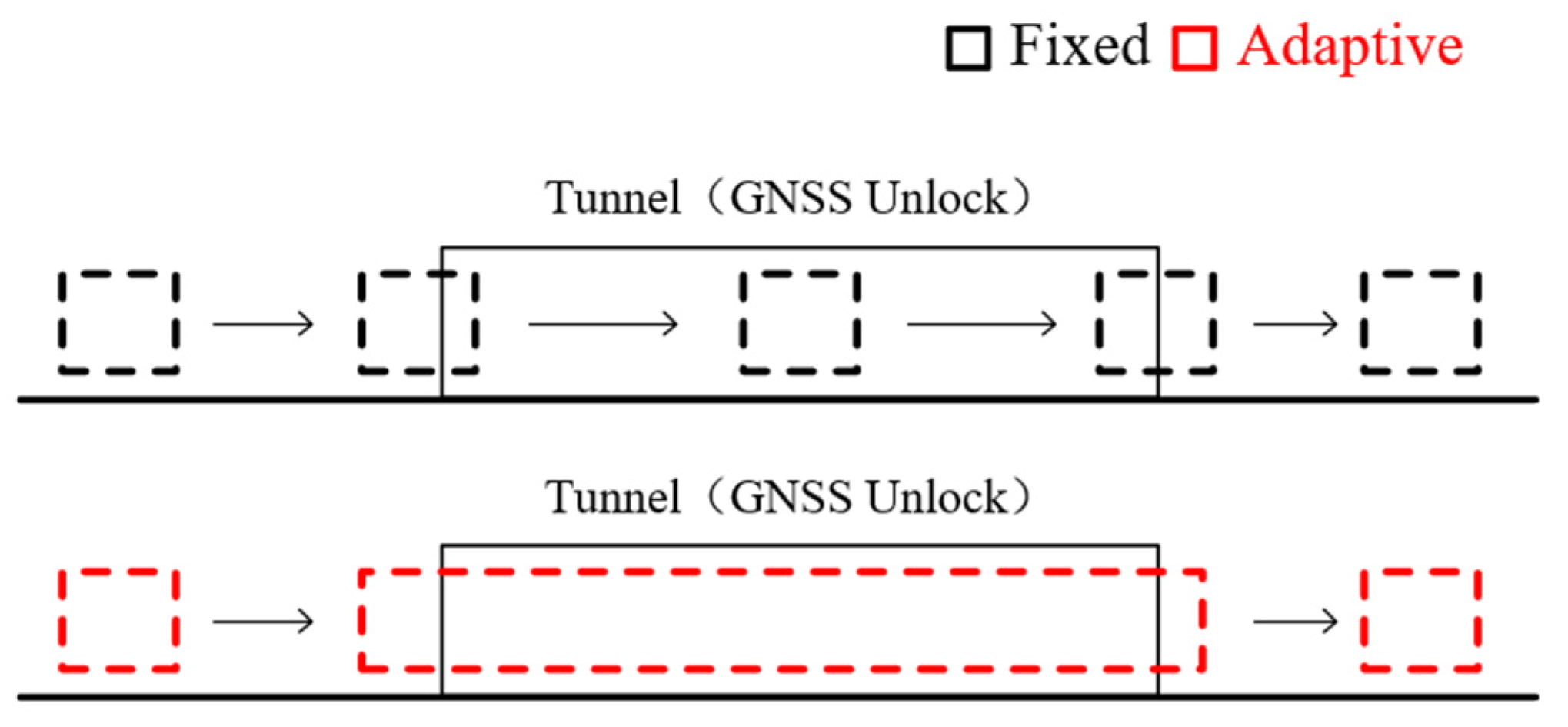
5. Adaptive Sliding Window

The conventional optimization process utilizing a fixed sliding window entails that when the number of states within the window reaches a predetermined length, the oldest state must be marginalized to accommodate a new one, with the window advancing by a constant step size of 1. This optimization approach can lead to a rapid decline in positioning accuracy if the GNSS out-of-lock duration exceeds the length of the window. While extending only the sliding window length may ensure positioning accuracy, it results in low computational efficiency. Consequently, we propose an adaptive window size adjustment scheme based on GNSS observation quality. Algorithm 1 for adjusting window size is detailed below, and its comparison with fixed sliding windows is illustrated in Figure 5.

Algorithm 1: Adaptive sliding window length adjustment

Input: window_size, init_length

1      init_length = n; 2      if No valid GNSS at front of window 3      window_size = window_size + 1; 4      else if Num of GNSS in window == init_length 5              marginalize 6        else if Num of GNSS in window > init_length 7                    Multistate marginalize 8                    window_size = init_length

The adaptive sliding window scheme enhances the window length to improve accuracy during GNSS unlock and promptly reduces the window length when excessive duration adversely affects computational efficiency. Unlike fixed-length sliding windows, the process of reducing window length necessitates the marginalization of multiple states, thereby requiring a multi-state marginalization algorithm to effectively implement the adaptive sliding window scheme.

When a fixed-length window transitions into a new state, it marginalizes the oldest point within that window and formulates an optimization equation to establish its relationship with associated states, as illustrated in Equation (13).

$$\left[\begin{array}{cc}{\mathbf{H}}_a& {\mathbf{H}}_{\mathbf{b}}\\ {\mathbf{H}}_{\mathbf{b}}^T& {\mathbf{H}}_c\end{array}\right]\left[\begin{array}{c}\delta {\mathit{x}}_1\\ \delta {\mathit{x}}_2\end{array}\right]=\left[\begin{array}{c}{\mathbf{b}}_1\\ {\mathbf{b}}_2\end{array}\right]$$

(13)

where $\delta {\mathit{x}}_1$ represents the variable to be optimized while $\delta {\mathit{x}}_2$ denotes the variable within the window that exhibits a constrained relationship with ${\mathit{x}}_1$. The matrices H and b are constructed from the Jacobian matrix and residuals. To derive a solution that marginalizes ${\mathit{x}}_1$ while preserving its observational information, Schur’s complement elimination is employed [16]; both sides of Equation (13) are then multiplied by Schur terms.

$$\left[\begin{array}{cc}\mathbf{I}& 0\\ -{\mathbf{H}}_{\mathbf{b}}^T{\mathbf{H}}_a^{-1}& \mathbf{I}\end{array}\right]\left[\begin{array}{cc}{\mathbf{H}}_a& {\mathbf{H}}_{\mathbf{b}}\\ {\mathbf{H}}_{\mathbf{b}}^T& {\mathbf{H}}_c\end{array}\right]\left[\begin{array}{c}\delta {\mathit{x}}_1\\ \delta {\mathit{x}}_2\end{array}\right]=\left[\begin{array}{cc}\mathbf{I}& 0\\ -{\mathbf{H}}_{\mathbf{b}}^T{\mathbf{H}}_a^{-1}& \mathbf{I}\end{array}\right]\left[\begin{array}{c}{\mathbf{b}}_1\\ {\mathbf{b}}_2\end{array}\right]$$

(14)

$$\left({\mathbf{H}}_c-{\mathbf{H}}_{\mathbf{b}}^T{\mathbf{H}}_a^{-1}{\mathbf{H}}_{\mathbf{b}}\right)\delta {\mathit{x}}_2={\mathbf{b}}_2-{\mathbf{H}}_{\mathbf{b}}^T{\mathbf{H}}_a^{-1}{\mathbf{b}}_1$$

(15)

The above equation eliminates $\delta {\mathit{x}}_1$ while retaining its observation information. All factors related to $\delta {\mathit{x}}_1$ are equivalent to the prior factors of $\delta {\mathit{x}}_2$, and the corresponding residual and Jacobian matrix are solved by linearization [25].

When the adaptive sliding window shrinks, n − 1 states need to be marginalized, assuming that all states within the window represent the optimal solution and all factors remain unchanged. Since each state is only related to its preceding and following states, n optimization equations are established accordingly.

$$\begin{array}{c}\left[\begin{array}{cc}{\mathbf{H}}_{11}& {\mathbf{H}}_{12}\\ {\mathbf{H}}_{12}^T& {\mathbf{H}}_{22}\end{array}\right]\left[\begin{array}{c}\delta {\mathit{x}}_1\\ \delta {\mathit{x}}_2\end{array}\right]=\left[\begin{array}{c}{\mathbf{b}}_1\\ {\mathbf{b}}_2\end{array}\right]\\ \left[\begin{array}{cc}{\mathbf{H}}_{22}^{\prime }& {\mathbf{H}}_{23}\\ {\mathbf{H}}_{23}^T& {\mathbf{H}}_{33}\end{array}\right]\left[\begin{array}{c}\delta {\mathit{x}}_2\\ \delta {\mathit{x}}_3\end{array}\right]=\left[\begin{array}{c}{\mathbf{b}}_2^{\prime }\\ {\mathbf{b}}_3\end{array}\right]\\ ⋮\\ \left[\begin{array}{cc}{\mathbf{H}}_{(\mathrm{n}-1)(\mathrm{n}-1)}^{\prime }& {\mathbf{H}}_{(\mathrm{n}-1)\mathrm{n}}\\ {\mathbf{H}}_{(\mathrm{n}-1)\mathrm{n}}^T& {\mathbf{H}}_{nn}\end{array}\right]\left[\begin{array}{c}\delta {\mathit{x}}_{n-1}\\ \delta {\mathit{x}}_n\end{array}\right]=\left[\begin{array}{c}{\mathbf{b}}_{n-1}^{\prime }\\ {\mathbf{b}}_n\end{array}\right]\end{array}$$

(16)

By marginalizing $\delta {\mathit{x}}_1$, the observed information of $\delta {\mathit{x}}_1$ is used as a prior factor for $\delta {\mathit{x}}_2$ and incorporated into the next optimization, resulting in a new optimized solution.

$$\left[\begin{array}{cc}{\mathbf{H}}_{22}^{\prime }+{\mathbf{H}}_{22}-{\mathbf{H}}_{21}{\mathbf{H}}_{11}{\mathbf{H}}_{12}& {\mathbf{H}}_{23}\\ {\mathbf{H}}_{23}^T& {\mathbf{H}}_{33}\end{array}\right]\left[\begin{array}{c}\delta {\mathit{x}}_2\\ \delta {\mathit{x}}_3\end{array}\right]=\left[\begin{array}{c}{\mathbf{b}}_2^{\prime }+{\mathbf{b}}_2-{\mathbf{H}}_{21}{\mathbf{H}}_{11}^{-1}{\mathbf{b}}_1\\ {\mathbf{b}}_3\end{array}\right]$$

(17)

Following the steps outlined above, ${\mathit{x}}_1,{\mathit{x}}_2,\cdots ,{\mathit{x}}_{n-2}$ are successively marginalized, leaving the optimization equations for the two states ${\mathit{x}}_{n-1},{\mathit{x}}_n$. Finally, the H-matrix and b-matrix, obtained through recursive updates, are used to marginalize ${\mathit{x}}_{n-1}$ using Equation (15). The observed information for ${\mathit{x}}_1,{\mathit{x}}_2,\cdots ,{\mathit{x}}_{n-1}$ is treated as a prior factor for ${\mathit{x}}_n$. This completes the marginalization of n − 1 points.

An adaptive sliding window is only used to ensure the accuracy of positioning when GNSS quality is poor, or GNSS is locked out. By increasing the window length when necessary, the computational complexity is proportional to the size of the window. Meanwhile, the multi-state marginalization algorithm can shorten the window length, reduce the computational complexity, and then strike a balance between accuracy and efficiency.

6. Test and Results

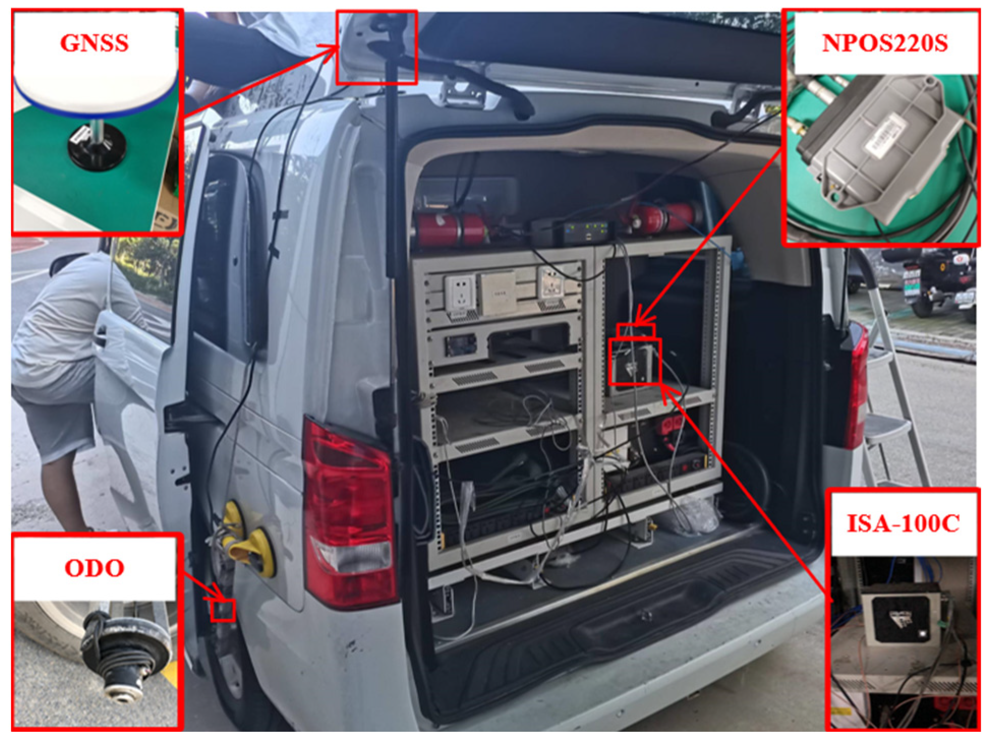
To verify the effectiveness of the proposed GNSS/IMU/ODO fusion navigation method based on an adaptive sliding window factor graph, a sports car test was conducted in a typical urban environment. The test results were then compared and analyzed. Data collected by the ISA-100C system was post-processed using IE as the ground truth. Figure 6 shows the test vehicle and equipment models as well as their installation.

The GNSS receiver and inertial navigation system are provided by the NPOS220S Integrated Navigation System, with the inertial navigation model being the OEM-IMU-EG320N. The system parameters are listed in

Table 1. IMU parameter.

Gyro 1 Bias	Gyro Random Walk	Acc 2 Bias	Acc Random Walk
$3.5°/\mathrm{h}$	$0.1°/\sqrt{h}$	0.1 mg	$0.05 m/s/\sqrt{h}$

¹ Gyro = Gyroscope. ² Acc = Accelerometer.

. The wheel odometer uses an encoder.

The sports car test scene, shown in Figure 7, includes complex environments such as underground garages, tall buildings, highways, and overpasses, ensuring the general applicability of the test results. Figure 7 also shows the test route.

6.1. Data Quality Analysis

Figure 8 displays the three-dimensional GNSS positioning standard deviation (STD) collected by the GNSS receiver. The analysis indicates a decrease in GNSS positioning accuracy around 500 s, with GNSS lockout occurring between 850 s and 1100 s. Due to the use of network RTK solutions, the positioning accuracy at other times remains high, typically less than 0.1 m.

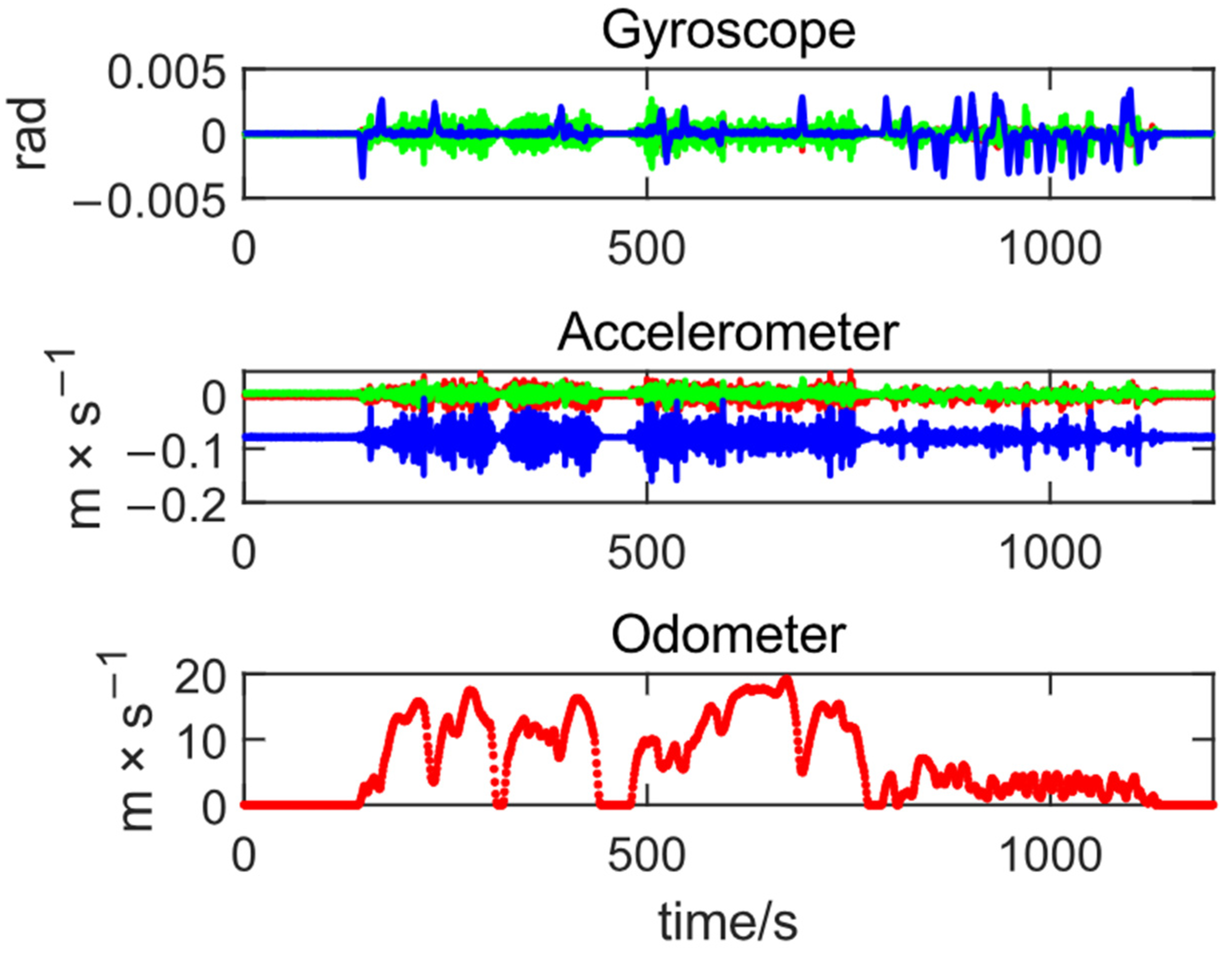
It is evident that under complex urban conditions, the quality of GNSS observations is unstable, with the longest recorded lockout time being 193 s. Figure 9 illustrates the data collected from inertial navigation and wheel speed measurements, where the three colors represent the output of the three axes of the accelerometer and gyroscope. During the initial 0 to 180 s, the vehicle remains at rest before starting to move. The maximum speed achieved is less than 20 m/s, and the vehicle comes to a stop for a period at the end of the test. Due to this initial static phase, GNSS cannot effectively constrain the carrier’s attitude [26], leading to various inertial navigation errors that cannot be effectively converged. Therefore, the initial pose data from this period will not be included in the subsequent pose error analysis.

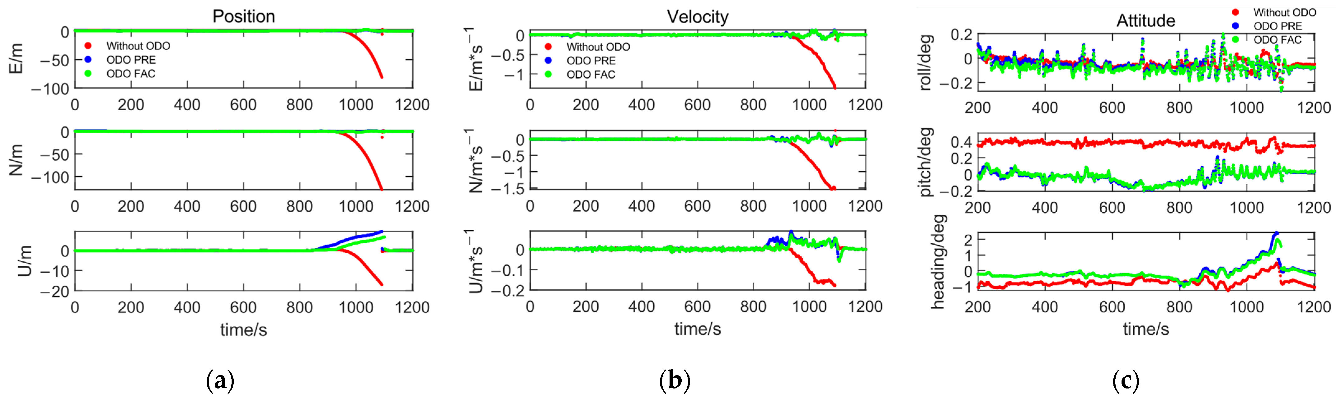
6.2. ODO as Factor

The test data of ODO were utilized as factors and pre-integrals in factor graph fusion and compared with the fusion process that excluded the ODO. The discrepancies between the results of position, velocity, and attitude across three dimensions (ENU) were calculated by comparing them to the true values, as illustrated in Figure 10.

Table 2. The RMS of three methods (without ODO, ODO as pre-integrals, ODO as factors).

Methods	Position (m)			Velocity (m/s)			Attitude (°)
	E	N	U	E	N	U	Roll	Pitch	Heading
Without ODO	13.281	23.253	3.230	0.257	0.371	0.049	0.062	0.370	0.764
ODO as pre-integrals	0.707	0.472	2.760	0.026	0.031	0.020	0.080	0.080	0.511
ODO as factors	0.798	0.538	1.735	0.025	0.027	0.016	0.090	0.078	0.483

presents the Root Mean Square (RMS) values of the error results obtained from the three calculation methods throughout the entire duration of the movement.

Based on the analysis presented in Figure 10 and Table 2, it is evident that incorporating wheel odometer data effectively addresses the issue of error divergence in GNSS lock-out position results, leading to a significant improvement in pose accuracy. The pre-integration of ODO measurements requires interpolation using subsequent wheel speed values; however, when treated as a factor, the current wheel speed alone suffices for resolution. Notably, the ODO as a factor can achieve positioning accuracy comparable to that obtained through pre-integration without relying on post-time observations, thereby validating the real-time constraints on pose error.

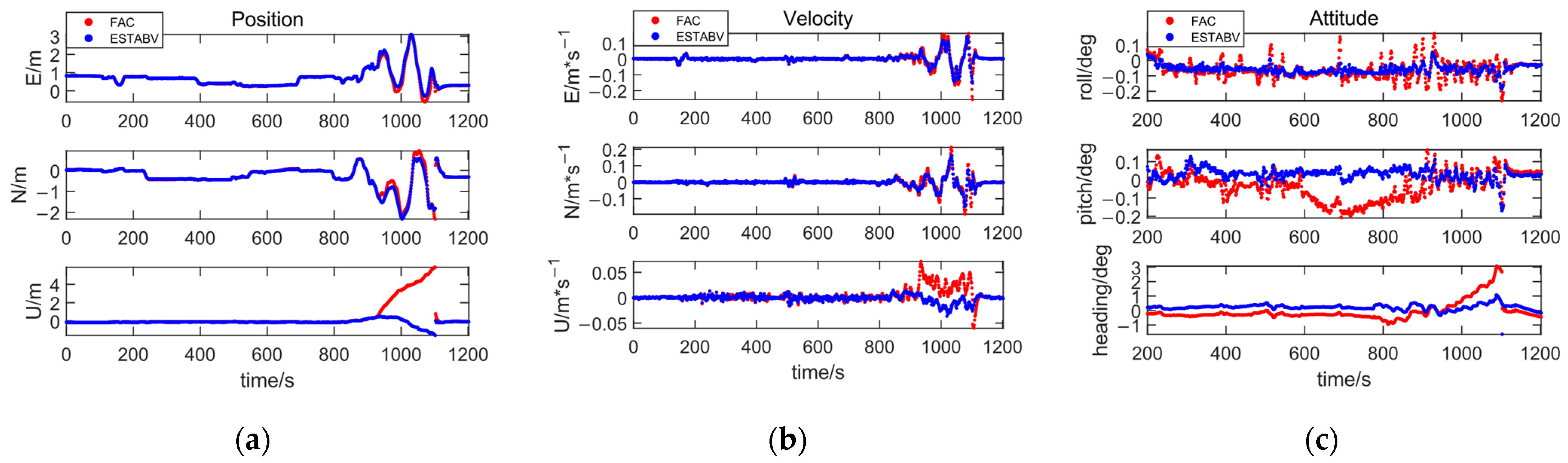
6.3. ODO Scale Factor and Installation Angle Estimation

In order to further improve the fusion accuracy of ODO and IMU, the ODO is used as a factor to solve the problem with and without installation angle, respectively, and the error results of position, speed, and attitude in three directions were obtained, as shown in Figure 11.

After introducing the installation angle estimation, the position error divergence in the elevation direction during the GNSS lockout period significantly decreased, with the absolute value dropping from 5.86 m to 1.56 m, a 73.4% reduction. Velocity accuracy also improved noticeably in the elevation direction during the GNSS lockout period, and the errors in the east and north directions were reduced as well. Additionally, attitude accuracy saw significant improvement, with more stable fluctuations. The RMS errors for both statistics are presented in

Table 3. The RMS of with and without installation angle.

Methods	Position (m)			Velocity (m/s)			Attitude (°)
	E	N	U	E	N	U	Roll	Pitch	Heading
Without Installation Angle	0.853	0.632	1.575	0.036	0.032	0.015	0.082	0.083	0.671
With Installation Angle	0.824	0.596	0.323	0.031	0.027	0.007	0.063	0.043	0.296

.

According to the analysis of Table 3, after introducing the installation angle estimation, the position error RMS in the elevation direction decreases by 43.8%, showing a significant improvement. The speed error RMS accuracy improves by 13.9%, 15.6%, and 53.3% in the three directions, respectively. Additionally, the accuracy of the roll, pitch, and heading angle RMS improves by 23.2%, 48.2%, and 55.9%, respectively, significantly enhancing the ability of wheel speed data to constrain the divergence of pose error during GNSS lockout.

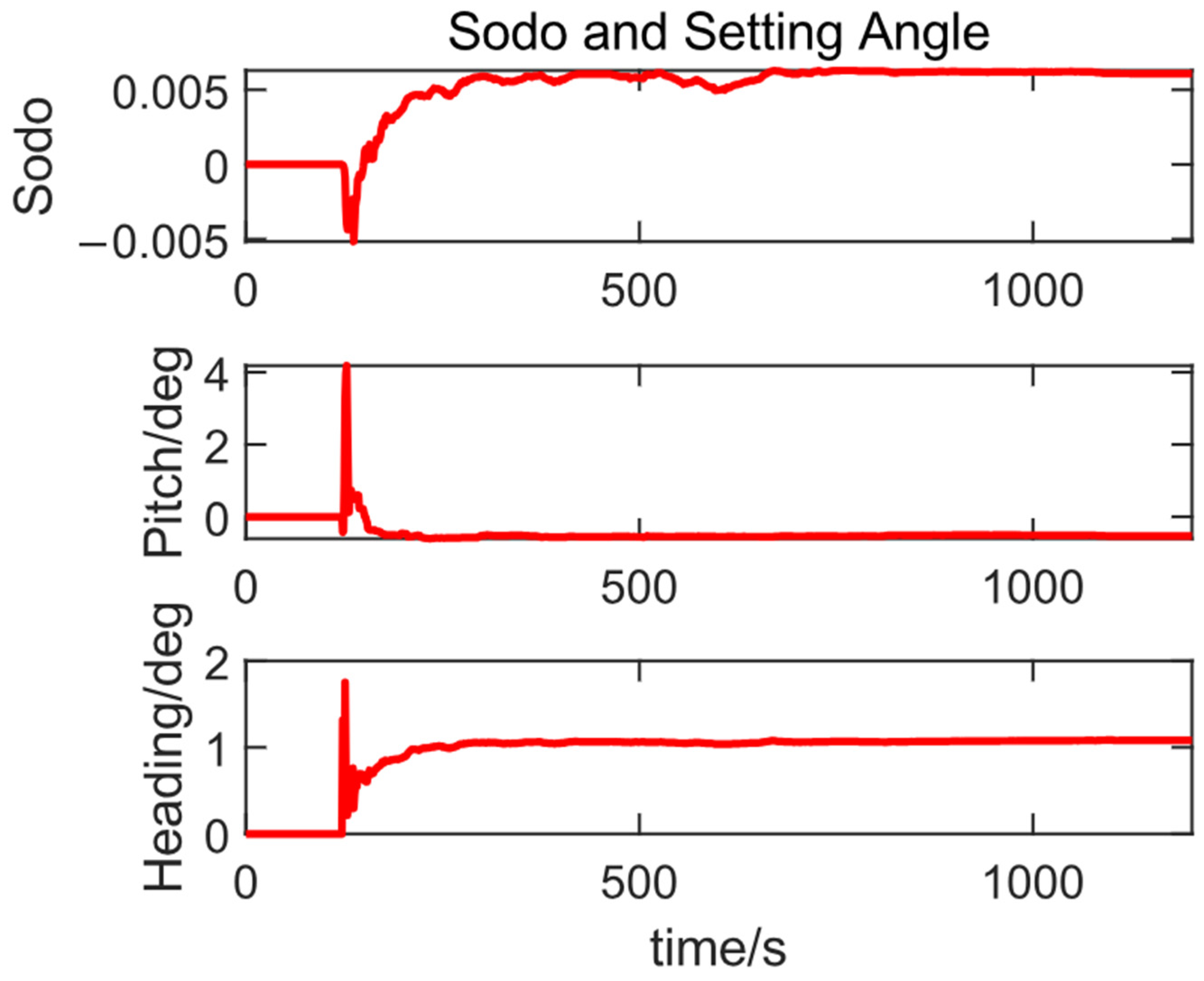
This demonstrates that adding the installation angle error reduces the divergence of GNSS position error in the elevation direction during the lockout and positively impacts speed and attitude accuracy. The estimated results for the ODO scale factor and installation angle are shown in Figure 12.

As can be seen from Figure 10, the estimated results of the three are basically correct and basically in a state of convergence. It can be obtained by calculating the mean value as the final estimated result that the scale factor of the ODO is 0.0059, the installation pitch angle is −0.53°, and the installation heading angle is 1.06°.

6.4. Adaptive Sliding Window Optimization Results

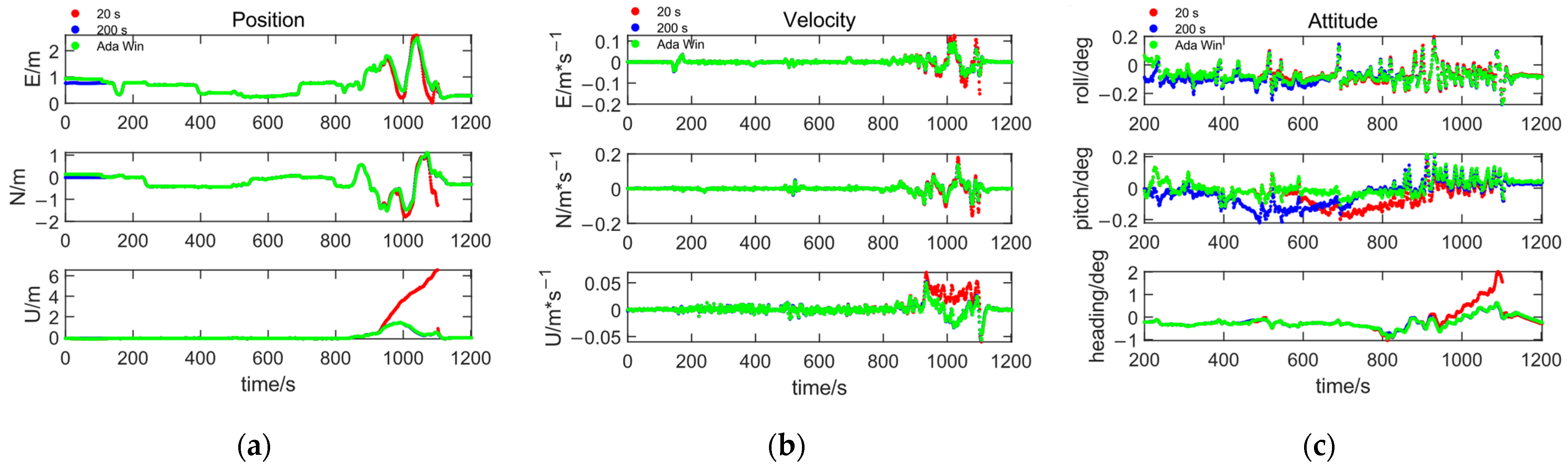
Based on the experimental data, factor graph fusion was performed using both fixed and adaptive sliding windows. The authors of [8] indicated that in typical urban environments, more accurate results are achieved when the window length reaches 20 s. Given that the longest lockout time in the test data was around 193 s, fixed sliding windows of 20 s and 200 s were used for fusion. The resulting position, velocity, and attitude errors are shown in Figure 13.

As shown in Figure 13, during periods when GNSS signals are available, the positioning accuracy across the three window types shows minimal difference. However, during GNSS lockout periods, the precision of the short window deteriorates significantly, with noticeable divergence, whereas the long window and adaptive sliding window maintain higher accuracy, producing smoother fusion pose results. To highlight the differences between the methods, the RMS values and fusion processing times during the GNSS lockout period were compared, as shown in

Table 4. The RMS and solution time of fixed and adaptive sliding window.

Methods	Position (m)			Velocity (m/s)			Attitude (°)			Time (s)
	E	N	U	E	N	U	Roll	Pitch	Heading
20 s-Fixed	1.382	1.017	3.924	0.056	0.059	0.035	0.101	0.075	0.825	32.62
200 s-Fixed	1.376	0.913	0.847	0.040	0.045	0.021	0.098	0.066	0.312	213.65
Adaptive	1.299	0.924	0.854	0.039	0.044	0.020	0.099	0.051	0.317	51.71

.

As shown in Table 4, the adaptive sliding window improves accuracy compared to the fixed 20 s window. The position error RMS decreases by 0.183 m, 0.093 m, and 3.070 m in the three directions, leading to an overall accuracy improvement of 55.3%. The velocity error RMS is reduced by 0.017 m/s, 0.015 m/s, and 0.015 m/s in the three directions, with an overall accuracy increase of 29.8%. For attitude error, the RMS is reduced by 0.002°, 0.024°, and 0.508°, with pitch and heading angle accuracy improving by 32.0% and 61.6%, respectively. Compared to the 200 s fixed window, the accuracy remains nearly the same, but the computation time is reduced by 161.94 s, boosting efficiency by 75.8%.

To validate the adaptability of the proposed method in different scenarios, we additionally gathered data from mountainous regions for analysis. As shown in Figure 14, the test route is more than 200 km, which includes complex GNSS signal conditions such as urban roads, mountain roads, multiple long tunnels, etc.

Given the suboptimal GNSS signal quality and prolonged loss of lock in such tunnels, the extended processing time required by the long-window method rendered it impractical. Consequently, only the short-window and adaptive sliding window methods were employed for data processing in these areas, with the results presented in Figure 15 and

Table 5. The RMS and solution time of fixed and adaptive sliding windows (mountainous regions).

Methods	Position (m)			Velocity (m/s)			Attitude (°)			Time (s)
	E	N	U	E	N	U	Roll	Pitch	Heading
20 s-Fixed	16.988	11.447	6.661	0.162	0.098	0.130	0.369	0.278	0.546	227.63
Adaptive	1.788	1.864	3.770	0.056	0.066	0.061	0.109	0.173	0.404	361.27

.

Due to the prolonged out-of-lock time of GNSS in mountainous regions, the position error of the short window has already shifted during the out-of-lock period. However, the adaptive sliding window scheme proposed in this paper maintains a relatively stable positioning performance. As illustrated in Table 4, compared to the 20 s short window, the adaptive sliding window scheme enhances the position accuracy in the three dimensions by factors of 89.5%, 83.7%, and 43.4%, the velocity accuracy in the three dimensions by factors of 65.4%, 32.6%, and 53.1%, and reduces the attitude errors in roll, pitch, and yaw by 70.5%, 60.8%, and 26.0%, respectively. This indicates that the proposed method can achieve precise and stable positioning results in mountainous environments.

In conclusion, the adaptive sliding window scheme not only enhances fusion navigation precision but also ensures computational efficiency, demonstrating the method’s effectiveness and superiority.

7. Conclusions

To address the issues of existing GNSS/INS/ODO fusion algorithms based on factor graphs, such as the asynchronous sampling frequencies of the IMU and wheel odometer and poor positioning accuracy during GNSS loss, an improved scheme is proposed. This approach incorporates the wheel odometer as a factor, estimates the installation angle, and utilizes an adaptive sliding window. The method was validated through real-world tests, with results showing that using the wheel odometer as a factor achieves positioning accuracy similar to pre-integration, eliminates the interpolation issues in high dynamic scenarios, and enhances the fusion algorithm’s potential for real-time application. Estimating the ODO scale factor and installation angle improves the ODO’s ability to constrain pose errors. The speed error RMS accuracy improves by 13.9%, 15.6%, and 53.3% in the three directions, respectively. Additionally, the accuracy of the roll, pitch, and heading angle RMS improves by 23.2%, 48.2%, and 55.9%. The adaptive sliding window scheme achieves better accuracy compared to a short window, achieving a 55.3% and 29.8% improvement in position and velocity accuracy and enhancements of 32.0% and 61.6% in pitch and heading angle accuracies, respectively. These results match the precision of long sliding windows, with a 75.8% gain in computational efficiency, demonstrating strong engineering applicability through an optimal balance of precision and efficiency. We also applied the method to the data in mountainous areas and obtained similar results.

The adaptive sliding window scheme dynamically adjusts the window size based on GNSS observation quality and directly uses GNSS positioning results for fusion. In the future, we will further improve the adaptability of GNSS in complex scenes by using pseudo-distance and pseudo-distance rates [27]. In addition, this process can be delayed when effective GNSS observations are unavailable during update intervals, which could slow down fusion optimization. In contrast, environmental features such as vision and point clouds can provide consistent observations within each update interval, ensuring the observability of the data in the window. Therefore, future work will integrate environmental features like vision and point clouds to further enhance the performance of the adaptive sliding window scheme.

References

- Xu, Z.; Yan, Z.; Li, X.; Shen, Z.; Zhou, Y.; Wu, Z.; Li, X. A Review of high-precision multi-source Fusion Localization for Intelligent Driving. Navig. Position. Timing 2023, 10, 1–20. [Google Scholar] [CrossRef]
- Angrisano, A. GNSS/INS Integration Methods. Ph.D. Thesis, Parthenope University of Naples, Naples, Italy, 2010. [Google Scholar]
- Gao, G.; Lachapelle, G. A Novel Architecture for Ultra-Tight HSGPS-INS Integration. Positioning 2008, 1, 13. Available online: http://www.scirp.org/journal/PaperInformation.aspx?PaperID=381&#abstract (accessed on 12 August 2024). [CrossRef]
- Kalman, R.E. A New Approach to Linear Filtering and Prediction Problems. J. Basic Eng. 1960, 82, 35–45. [Google Scholar] [CrossRef]
- Dellaert, F.; Kaess, M. Factor Graphs for Robot Perception. Found. Trends Robot. 2017, 6, 1–139. [Google Scholar] [CrossRef]
- Qin, T.; Li, P.; Shen, S. VINS-Mono: A Robust and Versatile Monocular Visual-Inertial State Estimator. IEEE Trans. Robot. 2018, 34, 1004–1020. [Google Scholar] [CrossRef]
- Wen, W.; Pfeifer, T.; Bai, X.; Hsu, L. Factor graph optimization for GNSS/INS integration: A comparison with the extended Kalman filter. Navigation 2021, 68, 315–331. [Google Scholar] [CrossRef]
- Wen, W.; Bai, X.; Kan, Y.C.; Hsu, L.-T. Tightly Coupled GNSS/INS Integration via Factor Graph and Aided by Fish-Eye Camera. IEEE Trans. Veh. Technol. 2019, 68, 10651–10662. [Google Scholar] [CrossRef]
- Chi, C.; Zhang, X.; Liu, J.; Sun, Y.; Zhang, Z.; Zhan, X. GICI-LIB: A GNSS/INS/Camera Integrated Navigation Library. arXiv 2023, arXiv:2306.13268v2. [Google Scholar] [CrossRef]
- Li, W.; Cui, X.; Lu, M. A robust graph optimization realization of tightly coupled GNSS/INS integrated navigation system for urban vehicles. Tsinghua Sci. Technol. 2018, 23, 724–732. [Google Scholar] [CrossRef]
- Zhang, Z.; Niu, X.; Tang, H.; Chen, Q.; Zhang, T. GNSS/INS/ODO/wheel angle integrated navigation algorithm for an all-wheel steering robot. Meas. Sci. Technol. 2021, 32, 115122. [Google Scholar] [CrossRef]
- Chang, L.; Niu, X.; Liu, T. GNSS/IMU/ODO/LiDAR-SLAM Integrated Navigation System Using IMU/ODO Pre-Integration. Sensors 2020, 20, 4702. [Google Scholar] [CrossRef] [PubMed]
- Zhao, H.; Ji, X.; Wei, D. Vehicle-Motion-Constraint-Based Visual-Inertial-Odometer Fusion with Online Extrinsic Calibration. IEEE Sensors J. 2023, 23, 27895–27908. [Google Scholar] [CrossRef]
- Park, K.-D.; Yoon, W.-J.; Lee, J.-S. Reduction of Multipath Effect in GNSS Positioning by Applying Pseudorange Acceleration as Weight. Sensors 2024, 24, 6880. [Google Scholar] [CrossRef] [PubMed]
- Zhang, X.; Wang, X.; Liu, W.; Tao, X.; Gu, Y.; Jia, H.; Zhang, C. A reliable NLOS error identification method based on LightGBM driven by multiple features of GNSS signals. Satell. Navig. 2024, 5, 31. [Google Scholar] [CrossRef]
- Niu, X.; Dai, Y.; Liu, T.; Chen, Q.; Zhang, Q. Feature-based GNSS positioning error consistency optimization for GNSS/INS integrated system. GPS Solut. 2023, 27, 89. [Google Scholar] [CrossRef]
- Leutenegger, S.; Lynen, S.; Bosse, M.; Siegwart, R.; Furgale, P. Keyframe-based visual–inertial odometry using nonlinear optimization. Int. J. Robot. Res. 2015, 34, 314–334. [Google Scholar] [CrossRef]
- Jiang, J.; Niu, X.; Liu, J. Improved IMU Preintegration with Gravity Change and Earth Rotation for Optimization-Based GNSS/VINS. Remote Sens. 2020, 12, 3048. [Google Scholar] [CrossRef]
- Tang, H.; Niu, X.; Zhang, T.; Fan, J.; Liu, J. Exploring the Accuracy Potential of IMU Preintegration in Factor Graph Optimization. arXiv 2022, arXiv:2109.03010. [Google Scholar] [CrossRef]
- Qin, T.; Cao, S.; Pan, J.; Shen, S. A General Optimization-based Framework for Global Pose Estimation with Multiple Sensors. arXiv 2019, arXiv:1901.03642. [Google Scholar] [CrossRef]
- De Maesschalck, R.; Jouan-Rimbaud, D.; Massart, D.L. The Mahalanobis distance. Chemom. Intell. Lab. Syst. 2000, 50, 1–18. [Google Scholar] [CrossRef]
- Wang, Y. Gauss–Newton method. WIREs Comput. Stat. 2012, 4, 415–420. [Google Scholar] [CrossRef]
- Ceres Solver—A Large Scale Non-Linear Optimization Library. Available online: http://ceres-solver.org/ (accessed on 9 October 2024).
- He, Q.; Chang, L.; Wu, Y. IMU/ODO External parameter estimation Based on Pre-integration. Bull. Surv. Mapp. 2021, 4, 68–73. [Google Scholar] [CrossRef]
- Engel, J.; Koltun, V.; Cremers, D. Cremers. Direct Sparse Odometry. IEEE Trans. Pattern Anal. Mach. Intell. 2018, 40, 611–625. [Google Scholar] [CrossRef] [PubMed]
- Liu, X.; Liu, Y.; Wen, C.; Li, Z. GNSS/SINS Integrated Navigation Algorithm in Complex Urban Environment. J. Electron. Inf. Technol. 2023, 45, 4150–4160. [Google Scholar]
- Rakhmanov, A.; Wiseman, Y. Compression of GNSS Data with the Aim of Speeding up Communication to Autonomous Vehicles. Remote Sens. 2023, 15, 2165. [Google Scholar] [CrossRef]
Figure 1.
General framework of the algorithm.
Figure 2.
GNSS/IMU/ODO fusion algorithm based on a factor graph.
Figure 3.
Factor graph fusion algorithm using ODO as a factor.
Figure 4.
The lever arm and installation angle.
Figure 5.
Fixed window and adaptive window.
Figure 6.
Test Vehicle and Equipment Installation.
Figure 7.
Test route and scene.
Figure 8.
GNSS positioning accuracy (B: latitude, L: longitude, H: height).
Figure 9.
Dataset of IMU and ODO.
Figure 10.
Error of without ODO, ODO as pre-integrals, ODO as factors: (a) Position; (b) Velocity; (c) Attitude. (E: East, N: North, U: Up).
Figure 11.
Error of with and without installation angle: (a) Position; (b) Velocity; (c) Attitude. (FAC: without installation angle, ESTABV: with installation angle).
Figure 12.
ODO scale factor and installation angle.
Figure 13.
Error of fixed and adaptive sliding window: (a) Position; (b) Velocity; (c) Attitude.
Figure 14.
Mountainous region test route.
Figure 15.
Error of fixed and adaptive sliding window (mountainous regions): (a) Position; (b) Velocity; (c) Attitude.