Research on Indoor Multi-Scene Base Station Deployment Method Based on HDOP

Abstract

In indoor positioning scenarios, the deployment of base stations plays a crucial role in the accuracy of positioning information. In recent years, how to reasonably deploy base stations to reduce HDOP (horizontal dilution of precision) has become a hot topic in the field of indoor positioning research. Currently, most research focuses only on HDOP in a specific indoor scenario and is often limited to simulation experiments, leaving room for further investigation. This paper conducts research on HDOP in multiple scenarios based on measured data. Firstly, the theoretical minimum value of HDOP is calculated for different numbers of base stations. Then, the relationship among the number of base stations, deployment methods, and HDOP is studied. Finally, an experimental platform is set up to analyze the relationship between HDOP and positioning errors based on measured data. The experimental results are as follows: (1) in simulated experiments in circular scenarios, the optimal deployment method entails evenly distributing the base stations around the circumference, with the deployment of an additional base station possibly reducing the average HDOP by about 10%, (2) in rectangular scenarios, the optimal deployment method entails evenly deploying the base stations along the two long sides. Measured data show that positioning errors are roughly proportional to the HDOP, but there are exceptions, and the reasons are analyzed. This research provides reference and support for the deployment of base stations in multi-scene indoor positioning systems.

1. Introduction

Global navigation satellite systems (GNSSs) have the advantages of high accuracy and wide coverage. At present, they can provide continuous, reliable, and all-weather integrated PNT (positioning, navigation and timing) services for global users outdoors [1]. However, due to the limited penetration capability of satellite signals and their susceptibility to obstruction, it is challenging for satellite signals to penetrate indoor environments. The signal strength indoors often does not support high-precision positioning. Therefore, achieving high-precision indoor positioning requires indoor positioning methods [2]. In recent years, with the change in lifestyle habits whereby many individuals spend most of their time indoors, the demand for high-precision indoor positioning systems has been steadily increasing. This trend has led to the emergence of various indoor positioning technologies, including pseudo-satellite base station positioning systems, ultra-wideband (UWB) positioning systems, Wi-Fi positioning systems, and 5G positioning systems [3,4,5,6]. These technologies rely on observing pseudo-range or angle values to achieve indoor positioning.

The primary task of an indoor positioning systems is to deploy base stations indoors. The deployment of base stations as part of indoor positioning systems is crucial for positioning accuracy. The position and network topology of base stations directly influence the accuracy and coverage of the positioning information [7]. Therefore, reasonably deploying indoor base stations and constructing appropriate network topologies represent the primary considerations in the context of indoor positioning. According to the analysis methods of GNSSs to attain positioning accuracy in the context of three-dimensional positioning problems, accuracy can be characterized by analyzing GDOP (geometric dilution precision), while, in the context of two-dimensional plane positioning problems, the focus is mainly on HDOP. As an indicator of positioning accuracy, HDOP can effectively evaluate the performance of the positioning system and improve its accuracy and stability by optimizing the HDOP value.

In recent years, many scholars, both domestically and internationally have conducted research on DOP in relation to indoor positioning problems. Li Dehai et al. studied rectangular scenes, investigating the positioning effects under various network conditions and summarizing the network principles for base stations in rectangular scenes, providing strong support for the deployment of base stations in indoor positioning systems [8]. Yao Haiyun et al. studied the influence of different Wi-Fi station layouts on the final positioning accuracy and provided a numerical analysis model for accuracy degradation factors. Through comprehensive analysis, they identified certain characteristics of positioning source structures, inspiring the optimization of the positioning source deployment [9]. Wang Chuanyang introduced two types of GDOP minimization conditions based on whether clock errors were considered, and simultaneously introduced and analyzed the cone configuration of GDOP minimization [10]. Haige Chen et al. proposed a novel passive ranging scheme that calculates its relative position without transmitting any signals. Evaluation in three indoor spaces showed a positioning accuracy of 1–2 m for an area of 2241 square meters [11]. However, most current research focuses solely on HDOP in specific scenarios and often only conducts simulation experiments. There is a lack of experimental platforms utilizing real measured data to analyze the corresponding relationship between HDOP and positioning errors. These gaps call for further in-depth research.

The main contributions and innovations of this paper are as follows. It is a study on HDOP in the context of indoor positioning across multiple scenarios, coupled with an analysis of the relationship between HDOP and positioning errors using real measured data, an approach which is lacking in other relevant literature. Firstly, we calculate the minimum values of HDOP for different numbers of base stations. Next, through simulation experiments, we test the optimal base station deployment methods in rectangular and circular scenarios, analyzing the influence of different numbers and positions of base stations on the HDOP at various points within the entire area. Finally, we construct a rectangular experimental scene and study the relationship between HDOP and positioning errors using real measured data.

We observe that few articles conduct experiments to verify the relationship between HDOP and positioning error, although, theoretically, the complexity of an indoor scene, for example, the positioning of indoor walls and large pieces of furniture, can seriously affect the propagation of a positioning signal and the layout of the base station. Therefore, this paper aims to conduct such an experiment to verify the actual engineering behind the HDOP and positioning error in light of the theory of the closed loop and the experiment itself. This paper aims to provide a reference for the deployment of indoor positioning systems in multiple scenarios, visually demonstrating the correspondence between HDOP and positioning errors, better meeting the research needs of scholars investigating indoor precision positioning, and promoting the improvement and development of indoor positioning technologies.

2. Principle of Horizontal Dilution of Precision (HDOP)

The geometric accuracy factor is one of the indicators for measuring positioning accuracy. In terms of two-dimensional positioning, the main focus is on the horizontal accuracy factor HDOP. The smaller the HDOP value, the more ideal the geometric distribution of the base station [12]. The calculation of HDOP involves the geometric distribution of the base stations, that is, the angle of and positional relationship between the base stations and the receivers. It is influenced by many factors, including the number and location of the base stations [13]. Generally speaking, when there are a large number of base stations and their positions are evenly distributed, the HDOP value will be lower [14].

$${\rho }_i=\sqrt{{(x_i-x)}^2+{(y_i-y)}^2+{(z_i-z)}^2}+c\Delta t$$

(1)

Among them, $c$ is the speed of light, the term $(x,y,z)$ indicates the coordinates of the target point, the term $(x_i,y_i,z_i)$ indicates the coordinates of the $i$ th base station, ${\rho }_i$ is the pseudo distance between the target point and the $i$ th base station, and $\Delta t$ is the estimated clock deviation value.

By applying the Taylor expansion to Equation (1) at an approximate position $(x^{\ast },y^{\ast },z^{\ast })$, retaining only the first-order term, we can obtain the following:

$$\Delta {\rho }_i=a_{xi}\Delta x+a_{yi}\Delta y+a_{zi}\Delta z-c\Delta t$$

(2)

Writing Equation (2) in matrix form yields:

$$\Delta P=H\Delta X$$

(3)

Among them,

$$\begin{gathered} \Delta P=\left[\begin{array}{c}\Delta {\rho }_1\\ \Delta {\rho }_2\\ ⋮\\ \Delta {\rho }_n\end{array}\right],\Delta X=\left[\begin{array}{l}\Delta x\\ \Delta y\\ \Delta z\\ -c\Delta t\end{array}\right],H=\left[\begin{array}{cccc}{a}_{x1}& a_{y1}& a_{z1}& 1\\ a_{x2}& a_{y2}& a_{z2}& 1\\ ⋮& ⋮& ⋮& ⋮\\ a_{xn}& a_{yn}& a_{zn}& 1\end{array}\right] \\ {a}_{xi}={\displaystyle \frac{x_i-x}{r_i^{\ast }}},a_{yi}={\displaystyle \frac{y_i-y}{r_i^{\ast }}},a_{zi}={\displaystyle \frac{z_i-z}{r_i^{\ast }}},r_i^{\ast }=\sqrt{{(x_i-x^{\ast })}^2+{(y_i-y^{\ast })}^2+{(z_i-z^{\ast })}^2} \end{gathered}$$

Using the least squares method to solve Equation (3), the following can be obtained:

$$\Delta X={(H^{T}H)}^{-1}{H}^T\Delta P$$

(4)

Among them, ${(H^{T}H)}^{-1}$ is a symmetric matrix.

$${(H^{T}H)}^{-1}=\left[\begin{array}{cccc}{B}_{11}& B_{12}& B_{13}& B_{14}\\ B_{21}& B_{22}& B_{23}& B_{24}\\ B_{31}& B_{32}& B_{33}& B_{34}\\ B_{41}& B_{42}& B_{43}& B_{44}\end{array}\right]$$

(5)

The horizontal accuracy factor $\mathrm{H}\mathrm{D}\mathrm{O}\mathrm{P}=\sqrt{{{\mathrm{B}}_{11}}^{ 2}+{{\mathrm{B}}_{22}}^{ 2}}$.

From the calculation formula of the HDOP, it can be seen that the value of HDOP is only related to the angle between the line connecting the target location and the base station, that is, the HDOP value is only determined by the geometric relationship between the base station and the target location.

The smaller the HDOP value, the more ideal the geometric distribution of the base station and the higher the positioning accuracy. On the contrary, the larger the HDOP value, the greater the amplification of the distance measurement error by the geometric layout between the tested node and the base station and the lower the positioning accuracy.

According to the formula derived from reference [15], the minimum value of HDOP can be obtained as follows:

$$\mathrm{H}\mathrm{D}\mathrm{O}\mathrm{P}\ge \sqrt{{\displaystyle \frac{\mathrm{n}}{\mathrm{f}(\mathrm{n})}}}$$

(6)

$$f(n)={\displaystyle \frac{n}{4}}-{\displaystyle \frac{1}{4}}({\displaystyle \sum _{i=1}^n\cos 2{\alpha }_i{)}^2}$$

(7)

Among them, $n$ is the number of base stations and ${\alpha }_i$ is the angle between the line connecting the $i$ th base station and the target point and the horizontal direction.

According to Equations (6) and (7), the theoretical minimum values of HDOP corresponding to different numbers of base stations can be derived, as shown in

Table 1. Minimum HDOP values for different numbers of base stations.

Number of Base Stations	Minimum HDOP Value	Difference from the Previous Result
3	1.1547	0
4	1	0.1547
5	0.8944	0.1056
6	0.8165	0.0779
7	0.7559	0.0606
8	0.7071	0.0488
9	0.6667	0.0404
10	0.6325	0.0342
11	0.6030	0.0295
12	0.5774	0.0256

and Figure 1.

From Table 1 and Figure 1, it can be seen that the theoretical minimum value of HDOP is inversely proportional to the number of base stations, meaning that the HDOP can be reduced by increasing the number of base stations, but the growth rate is decreasing. When the number of base stations reaches a larger value, increasing the number of base stations makes the reduction in the minimum value of HDOP less significant, a phenomenon which is not worth the cost increase brought about by increasing the number of base stations. Therefore, when actually deploying base stations, a relatively balanced value should be found between cost and HDOP.

3. Experiment and Analysis

Firstly, this paper considers two common real-world scenarios, namely circular scenes and rectangular scenes, for indoor positioning simulation experiments. Circular scenes are often seen in circular squares, amphitheaters, and spherical astronomical observations. Rectangular scenes are commonly found in underground parking lots, shopping malls, office buildings, etc.

3.1. Circular Scene Simulation Experiment

This part of the experiment aims to analyze the impact of base station position and number on HDOP values in circular scenes.

Firstly, this paper selected the two most common deployment methods for circular scenes with five base stations for simulation experiments, aiming to test the deployment method with the smaller HDOP through simulation experiments. The two common methods of station deployment include: (1) five base stations evenly distributed around the circumference and (2) four base stations evenly distributed around the circumference, while another base station is placed in the middle of the circle.

The first station layout was obtained through the use of the particle swarm optimization (PSO) algorithm. The PSO algorithm is an optimization algorithm based on swarm intelligence, proposed by Eberhart and Kennedy in 1995 [16]. It is inspired by the foraging behavior of bird flocks and simulates their social behavior when searching for food. The PSO algorithm has been widely applied to many optimization problems owing to its simplicity, ease of implementation, and few parameters. The PSO algorithm requires setting a reasonable fitness function for iteration. In this paper, points are selected according to a certain density within the positioning area, and the average HDOP value of these points is used as the fitness function to find the base station distribution method that minimizes the average HDOP value of each point. The second base station layout was obtained by consulting the literature and by using the HDOP calculation formula, which may lead to a smaller HDOP. It is generally believed that the more evenly distributed the base stations are, the more symmetrical they are, meaning that the overall HDOP is smaller. By comparing these two methods, we aim to find the station layout method with the smallest HDOP in this scenario [17,18]. The PSO algorithm has a relatively low complexity, with an overall time complexity of $O(m^{\ast }n)$ and an overall space complexity of $O(n)$. Among them,$m$ is the number of iterations and $n$ is the number of particles.

In this paper, we develop simulation experiments to calculate the HDOP of each station deployment method across different scenarios. Here, we set up a circular test site with a radius of 100 m and selected several points within the circular site at a density of 50 points/m² for the experiments. The average HDOP of these points and the probability distribution of HDOP below a certain threshold were calculated. The calculation results are shown in

Table 2. HDOP simulation results for different deployment methods of five base stations.

	Station Deployment Method 1	Station Deployment Method 2
Average HDOP	0.904	0.927
HDOP lower than 0.9	45.11%	13.25%
HDOP lower than 0.95	99.46%	81.36%
HDOP lower than 1	100.00%	94.39%
HDOP lower than 1.05	100.00%	98.89%
HDOP lower than 1.1	100.00%	99.97%
HDOP lower than 1.15	100.00%	100.00%

and Figure 2, Figure 3 and Figure 4.

Figure 2 depicts the cumulative distribution function (CDF) of the HDOP for each deployment method. From Table 2 and Figure 2, it can be seen that the average HDOP of the first method of station layout was relatively small, at 0.904, and the HDOP of all points was lower than 1. The average HDOP of the second method of station deployment was relatively high, at 0.927, with approximately 94.39% of the points having an HDOP lower than 1.

The simulation results in Figure 3 and Figure 4 show the distribution of HDOP values at various locations calculated using the HDOP formula. The overall distribution of the HDOP values can be visually observed. Different depths of colors are used in the figure to indicate the magnitude of HDOP values at different locations. The right column in the figure indicates the HDOP values corresponding to the different colors. The closer the color is to dark blue, the smaller the HDOP value is, while the closer the color is to red, the larger the HDOP value is. It can be seen that the HDOP of the first method of base station deployment was generally smaller, and the points with larger HDOP values in both deployment methods appeared to be located in the area with smaller angles and shorter distances from a certain base station, presenting a fan-shaped area with larger HDOP values.

Next, we increased the number of base stations to six and analyzed the impact of base station location and number on HDOP values through simulation experiments. The two selected station deployment methods are: (1) six base stations evenly distributed around the circumference and (2) five base stations evenly distributed aroound the circumference, while another base station is placed in the middle. The other settings for the simulation experiment were the same as those used in the previous five-base simulations. The calculation results are shown in

Table 3. Simulation results of different station layout methods for six base stations in the circular scene.

	Station Deployment Method 1	Station Deployment Method 2
Average HDOP	0.821	0.835
HDOP lower than 0.82	52.63%	11.20%
HDOP lower than 0.84	97.93%	76.26%
HDOP lower than 0.86	99.96%	90.22%
HDOP lower than 0.88	100.00%	96.26%
HDOP lower than 0.9	100.00%	98.74%
HDOP lower than 0.92	100.00%	99.80%
HDOP lower than 0.94	100.00%	100.00%

and Figure 5, Figure 6 and Figure 7.

From Table 3 and Figure 5, it can be seen that the average HDOP of the first method of station layout was relatively small, at 0.821, and the HDOP of all points was lower than 0.88. The average HDOP of the second method of station deployment was relatively high, at 0.835, with approximately 96.26% of the points having an HDOP lower than 0.88. Compared to five base stations, the average HDOP of six base stations was found to be lower, decreasing by about 10%, indicating that increasing the number of base stations can effectively reduce the HDOP.

From Figure 6 and Figure 7, it can be seen that the HDOP of the first method of station layout was generally smaller. The points with larger HDOP values in both station layout methods also appeared to be located in the area with smaller angles and shorter distances from a certain base station, presenting a fan-shaped area with larger HDOP values. This conclusion is the same as that obtained in relation to five base stations.

In summary, when the positioning scene is circular, the deployment method associated with the minimum HDOP value entails evenly laying the base stations around the circumference. When the number of base stations is six, the average HDOP is 0.821, and the maximum value is only 0.88, indicating that this is a good choice for station deployment in practical engineering. HDOP can be effectively reduced by increasing the number of base stations. When the receiver in the positioning system is located in an area characterized by a small angle and short distance from a base station, this special geometric configuration can lead to a significant increase in HDOP values. Therefore, when designing a positioning system, it is necessary to consider the relative position between the receiver and the base station, and other auxiliary means can be added in the sector with larger HDOP values to minimize positioning errors to the greatest extent possible.

3.2. Rectangular Scene Simulation Experiment

Firstly, this paper selected four common site deployment methods among six base station scenarios for the simulation experiments, aiming to determine the best site deployment method for minimizing HDOP through simulation experiments. The four commonly used and relatively effective site deployment methods are as follows:

• Deployment along the long side: deployment of a base station at the midpoint of each of the two long sides of the rectangular scene, with the remaining base stations located at the four corners of the rectangle.
• Deployment along the short side: deployment of a base station at the midpoint of each of the two short sides of the rectangular scene, with the remaining base stations located at the four corners of the rectangle.
• Regular hexagon deployment: uniform deployment of six base stations along the edges of the rectangle, with the base stations connected to form a regular hexagon.
• Centralized base station deployment: deployment of a base station at the midpoint of one long side of the rectangle and deployment of another at the center position, with the remaining base stations located at the four corners of the rectangle.

The first station layout method was obtained by using the particle swarm optimization algorithm to obtain the optimal station layout method based on the average HDOP value of each point in the region as the fitness function. The other station layout methods were obtained by consulting the literature and by using the HDOP calculation formula, which may lead to a smaller HDOP. For each site deployment method, simulation experiments were conducted to calculate the HDOP, aiming to determine the site deployment method with the minimum HDOP through experimentation.

In this paper, we established a rectangular test site measuring 600 m in length and 300 m in width. Several points within the rectangular area were selected for experimentation based on a density of 10 points/m². The average HDOP of these points and the probability distribution of HDOP values below a certain threshold were calculated. The calculation results are shown in

Table 4. Simulation results of different site deployment methods for six base stations.

	Station Deployment Method 1	Station Deployment Method 2	Station Deployment Method 3	Station Deployment Method 4
Average HDOP	0.942	1.105	1.182	1.010
HDOP lower than 0.9	37.455%	9.788%	35.634%	7.956%
HDOP lower than 1	74.580%	32.639%	53.740%	51.403%
HDOP lower than 1.1	94.075%	49.120%	64.591%	83.864%
HDOP lower than 1.2	99.997%	69.492%	72.030%	97.793%
HDOP lower than 1.4	99.997%	96.922%	78.624%	99.997%
HDOP lower than 1.6	99.997%	99.997%	83.729%	99.997%
HDOP lower than 1.8	99.997%	99.997%	88.194%	99.997%
HDOP lower than 2	99.997%	99.997%	91.793%	99.997%
HDOP lower than 2.2	99.997%	99.997%	94.416%	99.997%
HDOP lower than 2.4	99.997%	99.997%	96.304%	99.997%
HDOP lower than 2.6	99.997%	99.997%	97.690%	99.997%
HDOP lower than 2.8	99.997%	99.997%	98.659%	99.997%
HDOP lower than 3	99.997%	99.997%	99.327%	99.997%

and Figure 8, Figure 9, Figure 10 and Figure 11. To avoid the influence of extremely rare outliers on the visualization of the data, the data points in Figure 8, Figure 9, Figure 10 and Figure 11 are all those with HDOP values lower than 5.

From Table 4, it can be seen that the average HDOP value for the first method of deployment was the smallest, at 0.942, with almost all points having an HDOP value lower than 1.2. The average HDOP for the third method of deployment was the largest, at 1.182, with approximately 72.03% of the points having an HDOP value lower than 1.2.

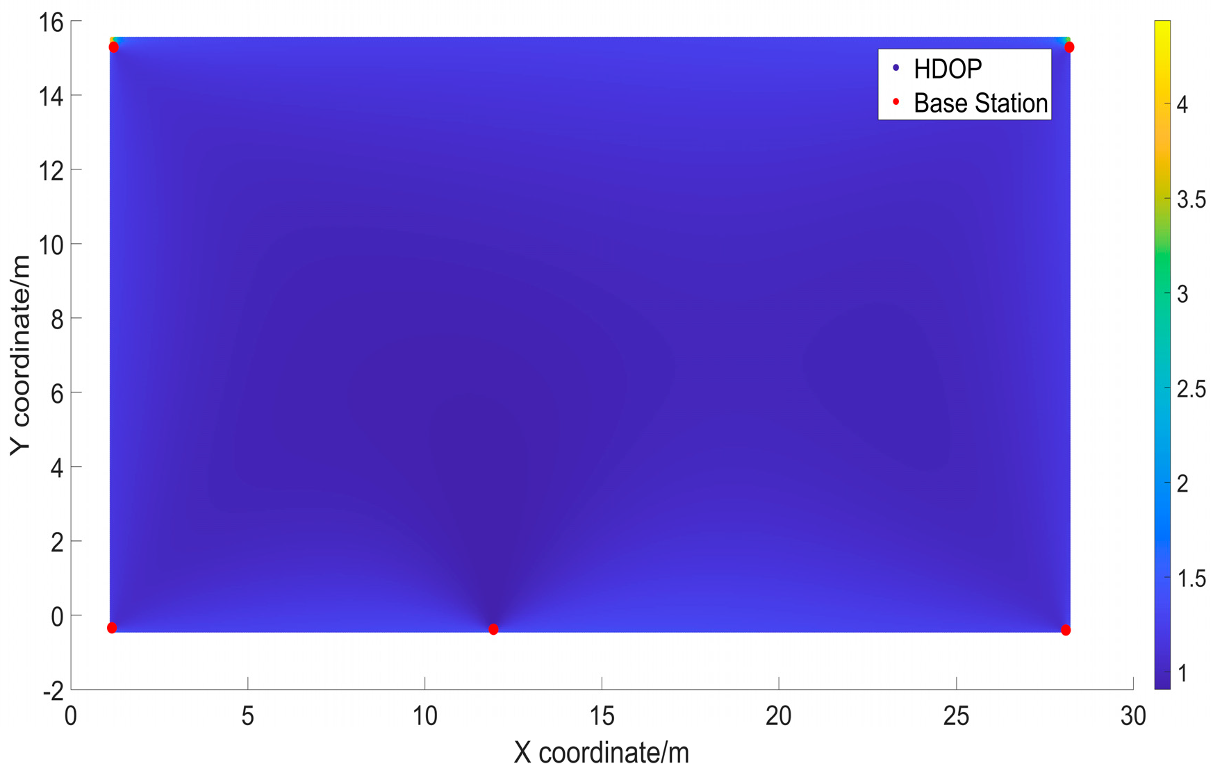
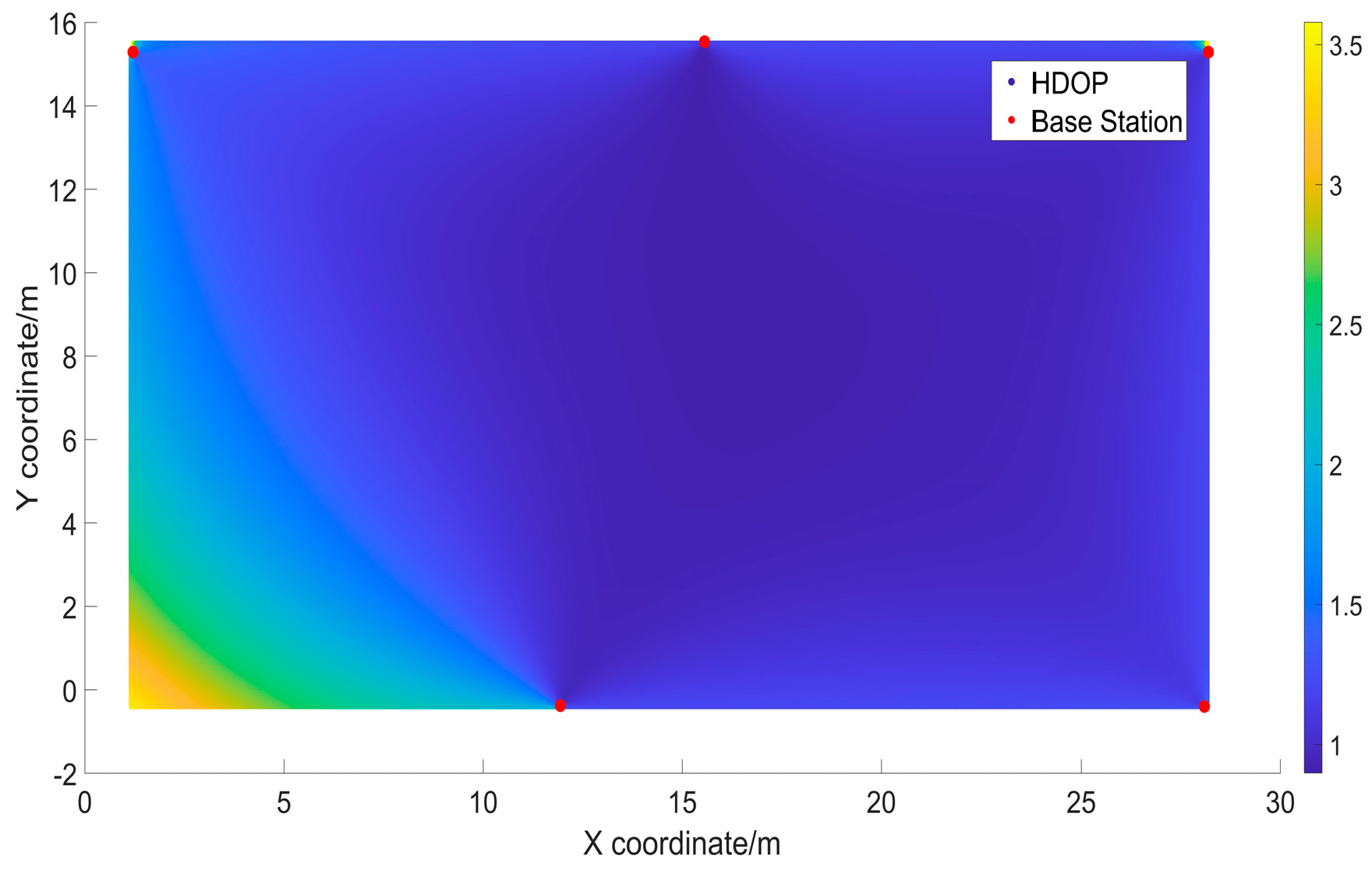
The simulated results in Figure 8, Figure 9, Figure 10 and Figure 11 depict the distribution of HDOP values calculated using the formula provided. This visualization offers a clear understanding of the overall HDOP distribution. The horizontal axis corresponds to the x-axis of the horizontal position, with a width of 600 m, while the vertical axis represents the y-axis of the horizontal position, with a width of 300 m. Different shades in the figures indicate the varying magnitude of HDOP values at different locations. The color bar on the right side of the graph indicates the corresponding HDOP values for each color, with darker blue representing lower HDOP values and lighter yellow indicating higher HDOP values.

It can be observed that the HDOP value for the first method of deployment was generally the lowest, indicating that appropriately increasing the spacing between base stations in a rectangular scenario can improve the distribution of HDOP values. Near the base stations, the colors in the images tend to be closer to dark blue, indicating lower HDOP values and, consequently, higher positioning accuracy. However, toward the edges of the x- and y-axes, corresponding to the edges of the test site, the colors tend toward the lighter yellow, suggesting higher HDOP values and potential positioning inaccuracies. The analysis in this study suggests that when the angle between a point and a base station decreases, as indicated by Equations (6) and (7), the value of $f(n)$ decreases. In such cases, the geometric configuration between the receiver and the base station becomes less favorable for HDOP, leading to an increase in HDOP values. Therefore, it might be beneficial to consider implementing additional measures at the edges of the rectangular area to reduce positioning errors.

From Figure 12, it is evident that the curve for the first method of deployment had the steepest slope, indicating that the majority of the points had lower HDOP values, with almost all points having HDOP values lower than 1.2. In contrast, the slope of the curve for the fourth method of deployment changed at a slower rate, indicating that this method generally results in higher HDOP values across all points, with more outliers or extreme points.

In summary, based on the simulation experiment in a rectangular scenario with six base stations, in a rectangular scene, the optimal base station deployment plan for six base stations entails their deployment at the four vertices and in the middle of the two long sides.

Circular and rectangular are the two most common scenarios in indoor positioning, but other irregular shapes may be encountered in practical engineering. Therefore, this article also provides the optimal base station distribution method for an ‘L’-shaped scenario. However, due to space limitations, this section only presents the optimal base station distribution method and does not show the comparison process with other station distribution methods like we did in relation to the rectangular and circular scenarios. In the ‘L’-shaped scenario, the optimal base station distribution with five and six base stations is shown in Figure 13 and Figure 14.

It can be seen from Figure 13 and Figure 14 that, in the ‘L’-shaped region, the average HDOP value at each point was inversely proportional to the number of base stations. The optimal station deployment strategy still prioritized vertices, with redundant base stations deployable on the edges to reduce the overall average HDOP.

3.3. Rectangular Scene Experimental Measurements

Finally, this paper established an experimental platform to analyze the relationship between HDOP and positioning error using real-world data. The specific experimental method involved selecting several combinations of base stations from six available ones, calculating the positioning error and HDOP for various points under each combination, and analyzing their corresponding relationship.

The tests were conducted in the basement of the aerospace city field area of the National Time Service Center of the Chinese Academy of Sciences. A rectangular indoor positioning scene was constructed in the basement, measuring approximately 30 m in length and 18 m in width. Six reinforced concrete pillars were installed in the middle, and six fixed UWB base stations were positioned accordingly. The testing scene and points are illustrated in Figure 15. In the figure, the yellow arrow lines represent the x-axis, the red arrow lines represent the y-axis, and the numbers denote the IDs of the testing points. The blue triangles indicate the positions of the UWB base stations, with the coordinates provided in

Table 5. Coordinates of the base stations in the simulated experimental rectangular scene.

	x-Coordinate/m	y-Coordinate/m
Base station 1	−0.34	1.16
Base station 2	−0.38	11.94
Base station 3	15.54	15.56
Base station 4	15.29	1.21
Base station 5	15.29	28.19
Base station 6	−0.4	28.09

.

It can be observed that there was a certain difference between the actual distribution of the base stations shown in Figure 15 and the theoretically optimal layout, mainly because the deployment height of the anchors depends on physical environmental factors such as building structures, walls, and obstacles, making it impossible for them to be installed in the theoretically optimal position. Therefore, in the actual deployment of the base stations, the optimal distribution of the base stations given in this article can be referred to, but adjustments should also be made based on the characteristics of the actual scenario.

This section aims to analyze the relationship between the positioning error and HDOP through experiments. Five base stations were selected from a pool of six for each experiment, resulting in six different station layout methods and corresponding HDOP scenarios. The objective is to examine the correlation between the positioning error and HDOP for each layout method.

Table 6. Combination of base stations in simulated rectangular scene experiment.

	Base Station Number
Combination 1	(1,2,3,5,6)
Combination 2	(1,2,4,5,6)
Combination 3	(1,2,3,4,5)
Combination 4	(1,2,3,4,6)
Combination 5	(1,3,4,5,6)
Combination 6	(2,3,4,5,6)

presents the combinations of the six layout methods.

Due to space limitations, 30 points were selected for the experiment. The average HDOP and the probability distribution of the HDOP values below a certain threshold for each deployment method at the 30 points were calculated. The calculation results are shown in

Table 7. HDOP calculation results for different combinations of five base stations.

Title 1	Combination 1	Combination 2	Combination 3	Combination 4	Combination 5	Combination 6
Average HDOP	1.288	1.211	1.264	1.049	1.044	1.178
HDOP lower than 1	32.002%	39.719%	33.616%	39.013%	41.813%	41.963%
HDOP lower than 1.2	62.454%	70.634%	66.598%	91.820%	92.901%	75.072%
HDOP lower than 1.4	73.769%	80.828%	77.078%	99.912%	99.915%	84.414%
HDOP lower than 1.6	81.026%	85.985%	82.987%	99.961%	99.956%	88.570%
HDOP lower than 1.8	86.142%	89.903%	87.263%	99.970%	99.968%	91.843%
HDOP lower than 2	90.586%	93.141%	90.978%	99.975%	99.975%	94.167%
HDOP lower than 2.2	93.877%	95.411%	93.858%	99.977%	99.975%	96.015%
HDOP lower than 2.4	96.066%	97.043%	95.957%	99.979%	99.977%	97.394%
HDOP lower than 2.6	97.588%	98.192%	97.440%	99.982%	99.979%	98.388%
HDOP lower than 2.8	98.642%	98.995%	98.489%	99.982%	99.979%	99.084%
HDOP lower than 3	99.343%	99.532%	99.204%	99.984%	99.982%	99.555%

and Figure 16, Figure 17, Figure 18, Figure 19, Figure 20 and Figure 21.

The simulation results in Figure 16, Figure 17, Figure 18, Figure 19, Figure 20 and Figure 21 depict the distribution of the HDOP values calculated by applying the HDOP formula at various locations. This provides an intuitive understanding of the overall HDOP distribution in the experimental scenario constructed in this paper. The vertical axis corresponds to the horizontal position on the x-axis, with a width of approximately 18 m, while the horizontal axis represents the horizontal position on the y-axis, with a width of about 30 m. Different shades of color in the graph indicate the magnitude of the HDOP values at each location. The bars on the right side of the graph indicate the HDOP values corresponding to different colors, where darker blue indicates smaller HDOP values and lighter yellow indicates larger HDOP values. From Table 7 and Figure 16, Figure 17, Figure 18, Figure 19, Figure 20 and Figure 21, it can be observed that combinations 4 and 5 exhibited uniform colors, approaching a deep blue, indicating very low HDOP values at each point with almost no outliers. Combination 1 had the highest average HDOP.

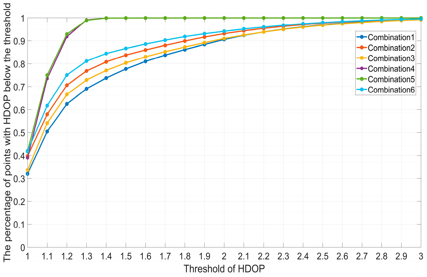
From Figure 22, it can be observed that the curves for combinations 4 and 5 had the steepest slopes, indicating that the HDOP values for the vast majority of the points were relatively small. Almost all points had HDOP values below 1.3. In contrast, the slope variation for the first method of base station deployment was the slowest, indicating that, when using this method, the HDOP values for each point were generally larger, suggesting the presence of more outliers or extreme points.

For combinations 4 and 5, an additional base station was deployed at the midpoint of the long side of the rectangle. Through actual measurement data verification, it was confirmed that these two deployment methods yielded the smallest HDOP values. This conclusion aligns with the findings of the earlier simulation experiments.

Finally, the relationship between the positioning error and HDOP was analyzed. In this study, the least squares method was used to calculate the position of the target point under different combinations of base stations, and the corresponding relationship between the average HDOP and the average positioning error was analyzed. The positioning errors for some target points under different combinations of base stations are shown in

Table 8. The positioning errors for some target points under different combinations of base stations.

Point Number	Positioning Errors for Combination 1/m	Positioning Errors for Combination 2/m	Positioning Errors for Combination 3/m	Positioning Errors for Combination 4/m	Positioning Errors for Combination 5/m	Positioning Errors for Combination 6/m
Point 2	0.325	0.058	0.367	0.094	0.047	0.115
Point 6	0.358	0.126	0.377	0.176	0.123	0.101
Point 10	0.328	0.087	0.089	0.083	0.068	0.120
Point 14	0.322	0.159	0.126	0.144	0.159	0.131
Point 19	0.399	0.139	0.417	0.192	0.137	0.114
Point 24	0.769	0.236	0.191	0.106	0.073	0.054
Point 27	0.362	0.171	0.319	0.149	0.146	0.148
Point 32	1.376	0.218	0.433	0.372	0.214	0.239
Point 37	0.510	0.218	0.140	0.167	0.119	0.101
Point 41	1.289	0.554	0.347	0.313	0.330	0.164
Point 45	1.159	0.389	0.328	0.248	0.269	0.067
Point 51	0.754	0.461	0.176	0.379	0.351	0.269
Point 54	0.518	0.203	0.181	0.187	0.120	0.103
Point 57	0.171	0.218	0.169	0.206	0.187	0.196
Average value	0.617	0.231	0.261	0.201	0.167	0.137

.

From Table 8 and Figure 23, it can be observed that among the 14 selected positioning points, the smallest average positioning error was achieved by base station combination 6, with an average positioning error of 0.137 m. The positioning error for almost all points was below 0.3 m. Combination 5 and combination 4 followed closely, with average errors of 0.167 m and 0.201 m, respectively. The positioning errors for almost all points were below 0.4 m. Combination 1 had the largest average positioning error.

The experimental results indicate that the positioning error was roughly proportional to HDOP, with a smaller HDOP leading to a smaller positioning error. However, there were exceptions. For instance, combination 6 had a higher HDOP than combination 5, but its average positioning error was smaller. This discrepancy might be due to the following reasons:

• HDOP is not the sole factor affecting positioning accuracy. Positioning accuracy is determined by two factors: DOP and user equivalent range error (UERE). UERE is a statistical quantity which represents the standard deviation of the distance error between the receiver’s measured results and the actual position. It considers various error sources, including base station location errors, receiver clock errors, multipath effects, and non-line-of-sight effects.
• Combination 6 had relatively higher HDOP values in the lower-left corner of the positioning area, where the x and y coordinates were smaller. However, a significant number of test points were not set in this area during the experimental testing. Therefore, the actual positioning error for combination 6 may be slightly higher than the average error of the tested points.
• The sample size of the 30 test points was relatively small, which may introduce some randomness, leading to statistical errors in positioning accuracy.
• There might be measurement errors in the actual coordinates of each positioning point.

4. Conclusions

The GNSS system can provide users with mature and stable positioning, navigation, and timing services in outdoor open areas around the clock. However, due to the weak penetration capability of satellite signals, it is difficult to receive navigation satellite signals indoors. Therefore, indoor positioning relies on other systems such as UWB and 5G distance-measuring base station positioning systems. How to reasonably deploy indoor base stations to reduce HDOP and, therefore, improve positioning accuracy has become one of the hottest research topics in the field of indoor positioning in recent years.

Most current research focuses solely on HDOP in specific scenarios and often only conducts simulation experiments. There is a lack of experimental platforms utilizing real measured data to analyze the corresponding relationship between HDOP and positioning errors. To address this issue, firstly, this study calculates the theoretical minimum value of HDOP for different numbers of base stations. Next, the study simulates common circular and rectangular scenarios, and through simulation experiments, analyzes the influence of different station layout methods and the number of base stations on HDOP in circular and rectangular scenarios. The simulation results show that in circular scenarios, the optimal station layout method consists of evenly distributing the base stations around the circumference, with the deployment of an additional base station possibly reducing the average HDOP by approximately 10%. The study also analyzes the reasons behind the higher HDOP values in certain regions. In rectangular scenarios, the optimal station layout method consists of evenly distributing the base stations along the two long sides. When the positioning points are close to the edges of the rectangular area formed by the base stations, the HDOP values increase rapidly, a phenomenon which is related to the angle between the point to be located and the base station. Finally, we set up real-world experimental scenarios and analyze the relationship between the positioning error and HDOP through measured data. The experimental results show that the positioning error is roughly proportional to HDOP, that is, a smaller HDOP results in smaller positioning errors. However, there are some exceptions. This paper provides analysis and explanations for them.

The work in of this paper aims to provide a reference for how to deploy base stations when designing indoor positioning systems. Through simulation experiments and the development of experimental scenarios, the study calculates and summarizes the influence of station layout methods on HDOP, analyzes the relationship between the positioning error and HDOP, and helps conduct in-depth research on indoor positioning issues. However, there are also shortcomings in this paper. Because of this limited attention that this topic have received, we did not find public open-source data sets. Moreover, the actual structures, such as the special round scene, were difficult to construct and the positioning of the equipment was difficult to attain, which is why our team was only able to construct a rectangular indoor scene for experimental purposes. Future research should include a wider range of experimental scenes or a larger data-set to improve the credibility of the results. This is one of the directions that we will follow in our future work.

References

- Li, B.; Miao, W.; Chen, G. Key Technologies and Challenges for High Precision Localization of Multi frequency and Multi mode GNSS. J. Wuhan Univ. (Inf. Sci. Ed.) 2023, 48, 1769–1783. [Google Scholar] [CrossRef]
- Jia, N.; Xue, C.; Yang, L.; Wang, Z. Robust Near Ultrasound Indoor Localization Method Based on Fusion Ensemble Learning. Comput. Res. Dev. 2024, 1–16. Available online: http://kns.cnki.net/kcms/detail/11.1777.TP.20240522.1343.008.html (accessed on 23 December 2024).
- Tang, W.; Chen, J.; Zhang, Y.; Ding, J.; Song, Z. Refined troposphere delay models by NWM ray-tracing for pseudolite positioning system and their performance assessment. Adv. Space Res. 2024, 73, 5017–5030. [Google Scholar] [CrossRef]
- Li, Z.; Fang, H.; Zhao, J.; Pang, L. A multi-node collaborative and iterative UWB localisation algorithm for indoor complex environments. Int. J. Sens. Netw. 2024, 44, 133–143. [Google Scholar] [CrossRef]
- Liu, J.; Deng, Z.; Hu, E. An NLOS Ranging Error Mitigation Method for 5G Positioning in Indoor Environments. Appl. Sci. 2024, 14, 3830. [Google Scholar] [CrossRef]
- SEl-Gendy, M.S.; Ashraf, I.; El-Hennawey, S. Wi-Fi Access Point Design Concept Targeting Indoor Positioning for Smartphones and IoT. Sensors 2022, 22, 797. [Google Scholar] [CrossRef] [PubMed]
- Wang, T.; Wu, J.; Jiao, X.; Zhu, J. Arrival time difference localization algorithm based on minimum HDOP station selection. J. Time Freq. 2021, 44, 183–196. [Google Scholar]
- Li, D.; Wu, W.; Ma, H.; Mi, J.; Zhao, J. Performance analysis of indoor ranging base station network positioning. J. Wuhan Univ. (Inf. Sci. Ed.) 2024, 1–12. [Google Scholar] [CrossRef]
- Yao, H.; Shu, H.; Sun, H.; Wang, S.; Zeng, K. DOP Numerical Analysis of WiFi Indoor Positioning Station Layout Optimization. Surv. Mapp. Geogr. Inf. 2022, 47, 34–38. [Google Scholar] [CrossRef]
- Wang, C. Research on UWB Positioning Method and Configuration Optimization. Ph.D. Thesis, China University of Mining and Technology, Beijing, China, 2020. [Google Scholar]
- Chen, H.; Dhekne, A. PnPLoc: UWB Based Plug & Play Indoor Localization. In Proceedings of the 2022 IEEE 12th International Conference on Indoor Positioning and Indoor Navigation (IPIN), Beijing, China, 5–8 September 2022; pp. 1–8. [Google Scholar] [CrossRef]
- Zhou, G.; Yang, L.; Liu, Z.; Ni, L. Analysis of the impact of TDOA based base station deployment on fuzzy area distribution and positioning accuracy. J. Nav. Eng. Univ. 2017, 29, 96–101. [Google Scholar]
- Zhang, S.; Yao, Z.; Lu, M. Fast deployment algorithm for ground-based pseudo satellite regional navigation system. J. Wuhan Univ. (Inf. Sci. Ed.) 2018, 43, 1355–1361. [Google Scholar] [CrossRef]
- Bai, M. Design and Localization Algorithm Research of Land-Based Multi-Point Positioning System Based on TDOA. Ph.D. Thesis, Chongqing University, Chongqing, China, 2010. [Google Scholar]
- Qian, Y.; Lu, M.; Feng, Z. Research on HDOP in ground positioning systems based on TDOA principle. Telecommun. Technol. 2005, 3, 135–138. [Google Scholar]
- Kennedy, J.; Eberhart, R. Particle swarm optimization. In Proceedings of the Proceedings of ICNN’95—International Conference on Neural Networks, Perth, WA, Australia, 27 November–1 December 1995; Volume 4, pp. 1942–1948. [Google Scholar] [CrossRef]
- Li, D.; Wei, S.; Gu, Z. Research on Optimization Design of Ground Wireless Positioning Base Station Deployment. Surv. Mapp. Sci. 2021, 46, 25–30. [Google Scholar]
- Wang, X. Research on Indoor Positioning Based on UWB Base Station Configuration. Ph.D. Thesis, Xi’an University of Electronic Science and Technology, Xi’an, China, 2014. [Google Scholar]
Figure 1.
Relationship between the HDOP theoretical minimum and number of base stations.
Figure 2.
CDF diagram of different station layout methods for five base stations in the circular area.
Figure 3.
HDOP associated with method 1 for the layout of five base stations.
Figure 4.
HDOP associated with method 2 for the layout of five base stations.
Figure 5.
CDF diagram of different station layout methods for six base stations in a circular area.
Figure 6.
HDOP diagram of deployment method 1.
Figure 7.
HDOP diagram of deployment method 2.
Figure 8.
HDOP for the first method of deployment.
Figure 9.
HDOP for the second method of deployment.
Figure 10.
HDOP for the third method of deployment.
Figure 11.
HDOP for the fourth method of deployment.
Figure 12.
CDF for different deployment methods of the six base stations.
Figure 13.
HDOP of the first layout method for the ‘L’-shaped scene.
Figure 14.
HDOP of the second layout method for the ‘L’-shaped scene.
Figure 15.
Schematic diagram of the test scene.
Figure 16.
HDOP distribution chart for combination 1.
Figure 17.
HDOP distribution chart for combination 2.
Figure 18.
HDOP distribution chart for combination 3.
Figure 19.
HDOP distribution chart for combination 4.
Figure 20.
HDOP distribution chart for combination 5.
Figure 21.
HDOP distribution chart for combination 6.
Figure 22.
CDF chart for different combination methods.
Figure 23.
CDF plot of positioning errors for different combination methods.