A Data–Physics-Driven Modeling Approach of Key Equipment for Large-Scale Distribution Network Simulation

Abstract

Fueled by pressing global climate concerns, the integration of large-scale renewable distributed generation sources, including distributed wind power and photovoltaics, along with electricity substitution loads into the distribution network has been accelerated to diminish carbon emissions. This shift introduces significant challenges and necessitates the advanced operation and control of distribution systems to accommodate these changes effectively. Against this backdrop, there is a growing expectation for an open and scalable central control mode, equipped with compatible interfaces, to offer a visionary development platform for the grid. This platform is anticipated to meet the evolving needs of future distribution system development, ensuring adaptability and forward compatibility. The aforementioned platform requires open, scalable, and interface-compatible models of key distribution network equipment as its foundation. To address the challenges presented, this paper proposes a data–physics-driven modeling approach for automating simulations in distribution systems. This method employs a simplified and standardized system of linear differential equations with undetermined coefficients to capture the common physical characteristics of specific device types. The models designed through this approach are notably open, allowing for real-time data to refine undetermined coefficients and accurately depict the dynamic behavior of equipment over various periods. Their scalability also stands out, rendering them apt for large-scale distribution network simulations. The paper elaborates on models for distributed photovoltaic, wind turbine, energy storage, and electric vehicle, and demonstrates their application within an IEEE-33 node distribution network topology built on Python.

1. Introduction

Motivated by global climate concerns, a significant integration of renewable distributed generation sources (such as distributed wind power and photovoltaic systems), along with electric substitution loads into the distribution network is underway to lower carbon emissions. This integration presents substantial challenges and necessitates the advanced application of operation and control systems within the distribution network [1,2,3]. On one hand, as the electricity substitution load increases, the economic losses and social impacts resulting from a single power outage have become increasingly difficult to manage. This situation underscores the necessity of equipping the distribution system with grid self-healing capabilities, leveraging local distributed generation to sustain power supply, especially for critical loads [4,5,6]. On the other hand, there is an expectation to employ advanced monitoring and control technologies in large-scale distributed generation to facilitate rapid and efficient demand response planning. This approach enables electric customers to actively engage in the electricity market, including participation in ancillary services like frequency and voltage regulation [7,8,9]. Furthermore, an open and extensible central control mode featuring compatible interfaces is anticipated to offer a progressive development platform for the grid. This platform should be capable of adapting to the evolving requirements of next-generation distribution system development. Consequently, automated simulation for the distribution system, encompassing functions such as monitoring, data exchange, and cooperative operation, forms the foundation for realizing these advanced applications.

Over the past few decades, the advent of IEC 61850 has established a standard framework for interoperability within power systems. It has progressively become one of the most critical communication protocols in power automation systems [10,11,12,13,14,15]. The object-oriented model structure characteristic of IEC 61850 offers a potential solution for device description in automated simulations of distribution systems. In the context of topology description and modeling of the distribution system, reference [16] introduces a method that utilizes the smart terminal unit (STU) to store local topology. This approach enables the achievement of static topology splicing and the recognition of contacting switches via STU communication. Similarly, reference [17] presents a distributed feeder control method grounded in local topology. This method leverages adjacent switches to convey information about available capacity and electrical distance, thereby aiding in the formulation of power supply recovery strategies. Reference [18] assigns specific static topologies to different functional levels of distributed Smart Terminal Units (STUs) and conducts dynamic topology processing. This enables the dynamic establishment of communication data flow connections among distributed STUs according to the real-time topology. Similarly, reference [19] introduces a distributed topology processing approach based on graph segmentation. This method employs communication between adjacent STUs to facilitate topology recognition within the ring network area.

In current research, considerable emphasis is placed on the topology description and modeling of distribution systems. However, there is a lack of detailed and universal modeling for distributed devices in the distribution network, such as distributed wind turbines, photovoltaic (PV) systems, energy storage, and electric vehicles supporting Vehicle-to-Grid (V2G) mode. The object-oriented modeling structure of IEC 61850 lacks the capability to depict the necessary dynamic characteristics of various devices. In recent years, the role of distributed energy resources in providing voltage and frequency support during fault transients in distribution networks has increasingly gained attention. Conversely, modeling methods based on detailed state space models in established commercial software, such as Matlab/Simulink, suffer from poor transferability among different device models, substantially increasing the modeling workload. This modeling methodology faces challenges in conducting dynamic simulations for the integration of distributed energy resources on a large scale within the distribution network. As a result, it is inadequate in facilitating the investigation of crucial issues essential to the distribution network’s stable and secure functionality. Such issues encompass the strategic placement and capacity planning for the integration of distributed energy resources, enhancement of control strategies for fault ride-through capabilities of distributed resources, identification of the distribution network’s vulnerabilities, and comprehension of fault progression within the network.

To reconcile the dilemma between the portability of models and their accuracy, particularly for facilitating dynamic simulations of extensive distributed energy resource integration within the distribution network, a novel data–physics-driven modeling approach for automated simulation of distributed generation systems has been introduced. This strategy employs a streamlined and uniform system of linear differential equations with adjustable coefficients to encapsulate the shared physical attributes of various device types. Consequently, this approach yields adaptable and universally applicable models that adeptly mirror the dynamic behavior of distributed energy resources within the distribution network. Distinguished by its adjustable parameters, uniform model interfaces, and an open modeling platform, this method has the ability of gathering real-time operational data to dynamically fine-tune parameters, achieving accurate replication of the dynamic features of devices. This technique substantially reduces the influence of nonlinear elements.

The remainder of this article is structured as follows: Section 2 delves into the proposed data–physics-driven modeling method, along with detailed modeling for various devices. Section 3 demonstrates the efficacy of this method through a case study within the context of the IEEE-33 node distribution network. Finally, conclusions are drawn in Section 4.

2. Proposed Data–Physics-Driven Modeling Method

2.1. Distributed Photovoltaic Model

In recent years, the scale of distributed photovoltaic (PV) power generation has seen significant growth, with its grid-connected capacity continuously expanding. This expansion has led to various impacts on the distribution network:

• The large grid-connected capacity of distributed PV leads to voltage violations in the distribution network.
• During grid faults, the disconnection of distributed PV results in power deficits, leading to a drop in system frequency. The residual dynamic voltage amplitude at distribution network nodes is low, causing a large number of users to lose power supply and affecting the quality of electricity supply.
• Different control strategies of distributed PV have an impact on the voltage and frequency of the distribution network during transient processes.

Therefore, developing the distributed PV model and implementing its dynamic simulation for integration into the distribution network has become a focal point of current research. By conducting dynamic simulations of distributed PV integration, the following objectives can be achieved:

• The integration of distributed PV systems into the distribution network dynamically impacts the voltage and frequency at the point of common coupling (PCC). The extent of this impact varies with the capacity and location of integration. Therefore, conducting a grid simulation of distributed PV models can assist in guiding the design of both the integration location and capacity of distributed PV systems.
• Simulating and quantifying the impact of various control strategies of distributed PV on the voltage and frequency of the distribution network during transient events, and analyzing the control strategy can ensure better performance in supporting the voltage and frequency of the distribution network during fault events, thereby guiding the refinement and enhancement of distributed PV control strategies.
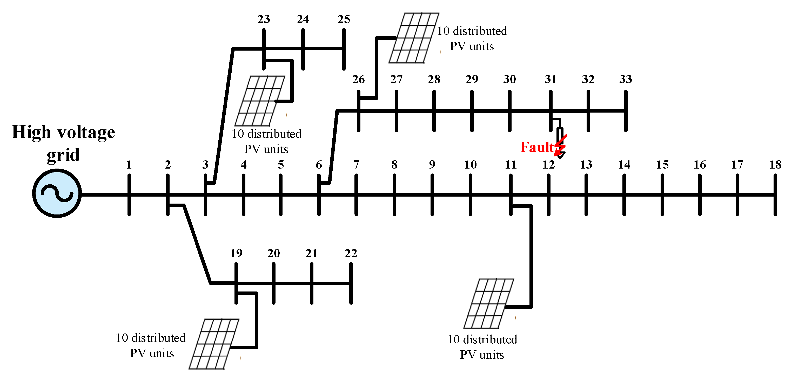
• This research implements dynamic simulations of distributed PV systems in the event of faults within the distribution network, particularly focusing on scenarios where system voltage and frequency experience drops due to short-circuit faults. Through dynamic simulations, the study examines the participation of distributed PV systems in fault ride-through and fault response, monitoring the resulting changes in system voltage and frequency. It delves into extreme scenarios that test the limits of distributed PV systems’ fault ride-through capabilities, such as incidents causing the voltage at the PCC of PV to fall below 0.2 per unit (p.u.) for longer than 0.15 s. Such conditions would necessitate the disconnection of distributed PV units from the grid, diminishing power support for the distribution network and potentially worsening fault situations. Investigating these extreme fault scenarios is pivotal for enhancing the strategies for prevention and mitigation of severe faults within the distribution network, as well as for refining emergency response plans for such incidents.

To meet the demands of large-scale simulations in distribution networks, we need to explore simplified and generic modeling methods for distributed PV. These modeling methods should retain critical dynamic behavior of distributed PV, such as active power control, reactive power control, dynamic voltage management, and dynamic frequency management. The modeling methods should effectively reflect the dynamic characteristics of distributed PV in large-scale simulations of distribution networks and enable dynamic analysis of multiple grid-connected PV. Furthermore, these methods should provide the benefits of flexibility in parameter adjustment and robust applicability.

As shown in Figure 1, the distributed PV model constructed in this paper is equipped with input sections such as the active power reference value (P_ref), external additional active power input (P_ext), reactive power reference value (Q_ref), and frequency reference value (F_{req_ref}). 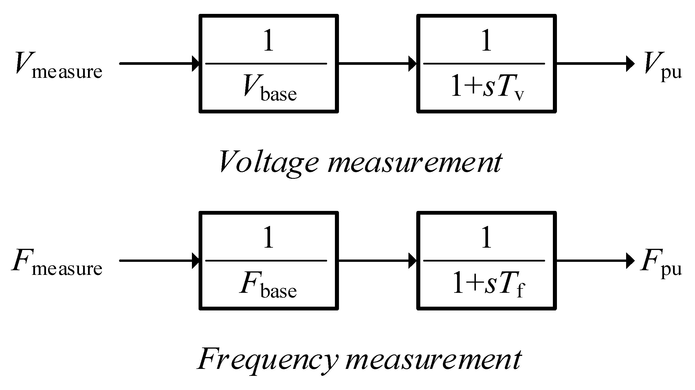It is connected to the distribution network through an external impedance X_c, with an output current (I_t) and voltage at the point of common coupling (V_t). In addition, the distributed PV model constructed in this paper is equipped with reactive power voltage compensation and active power frequency regulation functions. The implementation of these functions requires the distributed PV model to have the capability to measure both the voltage and frequency at the PCC.

2.1.1. The Reactive Power Voltage Compensation Function of the Distributed PV Model

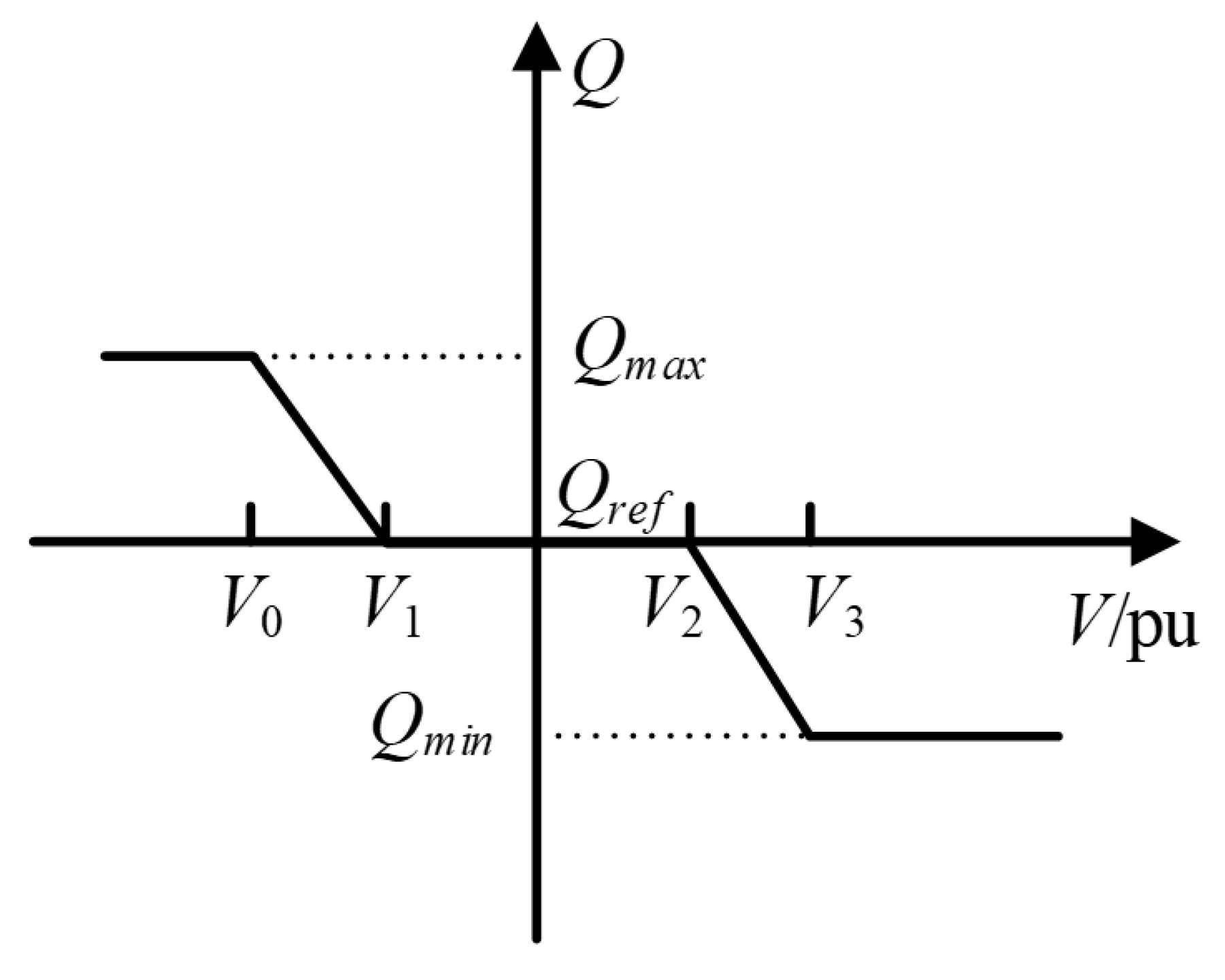
The Q(U) control strategy based on the voltage amplitude is realized by acquiring voltage information at the PCC (V_t). The reactive power reference value (Q) is obtained through the conversion of voltage information, and the control strategy is expressed as follows:

$$Q=\left\{\begin{array}{l}{Q}_{\max } V<V_0\\ \frac{Q_{\max }-Q_{ref}}{V_1-V_0}(V-V_1)+Q_{\max } V_0\le V\le V_1\\ Q_{ref} V_1<V\le V_2\\ \frac{Q_{ref}-Q_{\min }}{V_3-V_2}(V-V_3)+Q_{ref} V_2<V\le V_3\\ Q_{\min } V>V_3\end{array}\right.$$

(1)

In the formula, Q_max represents the maximum reactive power output of the inverter, and V₀, V₁, V₂, and V₃ are typically set to 0.95 p.u., 0.98 p.u., 1.02 p.u., and 1.05 p.u., respectively.

Figure 2 illustrates the droop curve under the Q(U) control strategy. From the figure, it is evident that when V > V₂, the reactive power output from distributed PV systems becomes increasingly smaller (generally negative), indicating that the distributed PV systems are absorbing inductive reactive power. When V > V₃, the reactive power absorbed by the distributed PV systems reaches its maximum. This maximum value is determined based on the inverter’s capacity to limit the rise in voltage at the PCC. Conversely, when V < V₁, the reactive power output from the distributed PV systems increases (generally positive), meaning that the distributed PV systems are supplying inductive reactive power to the distribution grid. When V < V₀, the reactive power supplied by distributed PV systems to the distribution grid hits its maximum. This maximum contribution is determined by the inverters’ capacities and is essential in reinforcing the voltage at the PCC, effectively counteracting voltage declines. The Q(U) control strategy fine-tunes the reactive power management of distributed PV systems in response to real-time voltage data at the grid interconnection, enabling every connected distributed PV system to actively engage in the dynamic voltage regulation of the distribution grid.

2.1.2. The Active Power Frequency Regulation Function of the Distributed PV Model

Primary frequency regulation at PV stations is mainly achieved through PV inverters. When the distributed PV’s measuring devices detect changes in the distribution network’s frequency, the distributed PV will adaptively adjust its output of active power through the active power frequency regulation function to respond to the instantaneous changes in the distribution network’s frequency. If the distribution network experiences a dip in frequency, distributed PV systems escalate their active power output to elevate the network’s frequency. Conversely, in instances where the network’s frequency is above the desired level, these systems curtail their active power contribution to decrease the frequency. This adaptive approach allows distributed PV systems to contribute effectively to the frequency regulation of the distribution network, playing a pivotal role in ensuring its secure and stable functionality.

The active power frequency regulation control strategy for distributed photovoltaics is articulated as follows:

$$P_{drop}=(F_{req\_ref}-F_{req})\times Ddn$$

(2)

In the formula, Ddn represents the coefficient for active power frequency regulation. When F_req < F_{req_ref}, this reflects a situation where the frequency detected at the PCC falls beneath the standard threshold, necessitating an augmentation of active power output from distributed photovoltaic systems. On the flip side, F_req > F_{req_ref} indicates a frequency at the PCC exceeding the norm, which prompts a decrease in the active power output from distributed photovoltaics.

Furthermore, the distributed photovoltaic model presented in this study introduces a sophisticated approach for managing both active and reactive current reference values. This is achieved through a dual control strategy that simultaneously considers voltage and frequency management at the PCC, underscoring a holistic framework for optimizing grid integration and operational performance.

Within this framework, the approach to voltage management is depicted in Figure 3, and the corresponding strategy can be described as follows:

$$\begin{array}{l}{F}_{vl}=K_{vt01}{z}_i^{VL1}(V-V_{to})+z_u^{VL1}\\ K_{vt01}=\frac{1}{V_{t1}-V_{t0}}\\ z_i^{VL1}=\left\{\begin{array}{l}1 V_{t0}\le \mathrm{V}\le V_{t1}\\ 0 \mathrm{V}\le V_{t0} \mathrm{or} V\ge V_{t1}\end{array}\right.\\ z_u^{VL1}=\left\{\begin{array}{l}1 V_{t1}\le \mathrm{V}\\ 0 \mathrm{V}\le V_{t1}\end{array}\right.\end{array}$$

(3)

$$\begin{array}{l}{F}_{vh}=K_{vt23}{z}_i^{VL2}(V-V_{t2})+z_l^{VL2}\\ K_{vt23}=\frac{-1}{V_{t2}-V_{t3}}\\ z_i^{VL2}=\left\{\begin{array}{l}1 V_{t2}\le \mathrm{V}\le V_{t3}\\ 0 \mathrm{V}\le V_{t2} \mathrm{or} V\ge V_{t3}\end{array}\right.\\ z_l^{VL2}=\left\{\begin{array}{l}1 V\le V_{t2}\\ 0 \mathrm{V}\ge V_{t2}\end{array}\right.\end{array}$$

(4)

When the voltage at the PCC of distributed photovoltaics falls within the low voltage range (V_t0 < V_t < V_t1), the low voltage section’s voltage pointer z_i^VL1 is set to 1 and z_u^VL1 to 0, with the voltage management coefficient F_vl being derived from Formula (3). Conversely, when the voltage at the PCC of distributed PV falls within the high voltage range (V_t2 < V_t < V_t3), the high voltage section’s voltage pointer z_i^VL2 is set to 1 and z_l^VL2 to 0, with the voltage management coefficient F_vh obtained from Formula (4). These voltage management coefficients, F_vl and F_vh, are integral to formulating both the active current reference (I_pcmd) and reactive current reference (I_qcmd), as illustrated in Figure 4. By employing these coefficients, a dynamic management framework for active and reactive current references is established, tailored to the voltage at the PCC of distributed PV systems.

In Figure 4, the meanings of the variables are presented in the

Table A1. The meaning of variables for distributed photovoltaics.

Variable	Description
$Q_{max}$	Maximum Reactive Power Command
$Q_{min}$	Minimum Reactive Power Command
$V_0$	Lower Deadband Limit for Voltage Droop Response
$V_1$	Upper Deadband Limit for Voltage Droop Response
$Dqdv$	Voltage Droop Response Characteristics
$V_{t0}$	Voltage Trip Response Curve Point 0
$V_{t1}$	Voltage Trip Response Curve Point 1
$V_{t2}$	Voltage Trip Response Curve Point 2
$V_{t3}$	Voltage Trip Response Curve Point 3
$F_{t0}$	Frequency Trip Response Curve Point 0
$F_{t1}$	Frequency Trip Response Curve Point 1
$F_{t2}$	Frequency Trip Response Curve Point 2
$F_{t3}$	Frequency Trip Response Curve Point 3
$T_g(I_p)$	Inverter Active Current Lag Time Constant
$T_g(I_q)$	Inverter Reactive Current Lag Time Constant
$V_t$	The Voltage at Point of Common Coupling
$P_{ref}$	Initial Active Power
$F_{req}$	The Frequency at Point of Common Coupling
$Q_{ref}$	Initial Reactive Power
$I_{pcmd}$	Active Current Command
$I_{qcmd}$	Reactive Current Command

at Appendix A.

The frequency management functionality of distributed photovoltaics is depicted in Figure 5, and the strategy can be described as follows:

$$\begin{array}{l}{F}_{fl}=K_{ft01}{z}_i^{FL1}(F-F_{to})+z_u^{FL1}\\ K_{ft01}=\frac{1}{F_{t1}-F_{t0}}\\ z_i^{FL1}={\left\{\begin{array}{l}1 {\mathrm{F}}_{t0}\le F\le F_{t1}\\ 0 \mathrm{F}\le F_{t0} \mathrm{or} \mathrm{F}\ge F\end{array}\right.}_{t1}\\ z_u^{FL1}=\left\{\begin{array}{l}1 {\mathrm{F}}_{t1}\le F\\ 0 \mathrm{F}\le F_{t1}\end{array}\right.\end{array}$$

(5)

$$\begin{array}{l}{F}_{fh}=K_{ft23}{z}_i^{FL2}(F-F_{t2})+z_l^{FL2}\\ K_{ft23}=\frac{-1}{F_{t2}-F_{t3}}\\ z_i^{FL2}=\left\{\begin{array}{l}1 {\mathrm{F}}_{t2}\le F\le F_{t3}\\ 0 \mathrm{F}\le F_{t2} \mathrm{or} \mathrm{F}\ge F_{t3}\end{array}\right.\\ z_l^{FL2}=\left\{\begin{array}{l}1 \mathrm{F}\le F_{t2}\\ 0 \mathrm{F}\ge F_{t2}\end{array}\right.\end{array}$$

(6)

When the frequency at the PCC of distributed PV falls within the low frequency range (F_t0 < F_req< F_t1), the low frequency segment’s frequency pointer z_i^FL1 is set to 1, and z_u^FL1 to 0, with the frequency management coefficient F_fl obtained from Formula (5). Conversely, when the frequency falls within the high frequency range (F_t2 < F_req < F_t3), the high frequency segment’s frequency pointer z_i^FL2 is set to 1, and z_l^FL2 to 0, with the frequency management coefficient F_fh determined by Formula (6). The frequency management coefficients, F_fl and F_fh, play a pivotal role in shaping the active current reference (I_pcmd) and reactive current reference (I_qcmd), as illustrated in Figure 4. Through this mechanism, a dynamic framework for adjusting active and reactive current references is established, rooted in the frequency at the PCC of distributed PV systems.

2.2. Energy Storage Model

Following the carbon peaking and carbon neutrality goals, there has been a remarkable surge in the development of new energy projects across diverse regions. China’s rich natural resources have enabled the widespread integration of distributed wind and solar PV systems into the distribution grid. However, the inherent sensitivity to environmental factors, coupled with the unpredictability and variability of distributed energy production, poses significant challenges to the stability, reliability, and power quality of the grid. Moreover, the increasing presence of nonlinear, impulsive loads and power electronics conversion devices further aggravates power quality concerns within the distribution grid.

Amid escalating interest in energy storage system research, the implementation of energy storage solutions to improve the power quality in the distribution grid has increasingly captivated academic attention. Energy storage systems disrupt the conventional instantaneous consumption and balance paradigm of power systems, offering rapid response and bi-directional control capabilities that facilitate frequency regulation, peak shaving, and improvement of power quality. Incorporating energy storage into the distribution grid strengthens its ability to integrate distributed energy resources, thereby optimizing resource distribution. Given this scenario, creating a versatile, adaptable energy storage model specifically designed for the distribution grid is essential for effective strategic planning and ensuring a secure, stable network operation.

The dynamic simulation of Integrating energy storage models into the distribution grid offers valuable insights into the optimal grid connection capacities for energy storage systems. This process facilitates a comprehensive analysis of how the combined integration of distributed photovoltaics and energy storage can enhance the distribution grid’s resilience to transient voltage fluctuations, frequency stability, and overall power quality. Moreover, it enables an exploration of the beneficial effects that the integration of energy storage systems has on the distribution grid’s capacity to accommodate distributed energy resources effectively.

The energy storage system model presented in this study integrates essential dynamic elements, including active power control, reactive power control, dynamic voltage regulation, and charge state management. It is capable of effectively reflecting the dynamic characteristics of energy storage systems in large-scale distribution grid simulations, facilitating dynamic analysis of energy storage integration into the grid.

Figure 6 illustrates the energy storage model established in this paper, which is divided into an electrical control part and a current converter part. The electrical control part receives external commands for active power reference value (P_ref), power factor angle reference value (P_faref), external reactive power reference value (Q_ext), and voltage reference value (V_ref0). I_t also measures the voltage at the energy storage system’s PCC (V_t), the active power output from the energy storage (P_elec), and the reactive power output (Q_elec). This enables the setting of the active current reference value (I_pcmd) and the reactive current reference value (I_qcmd).

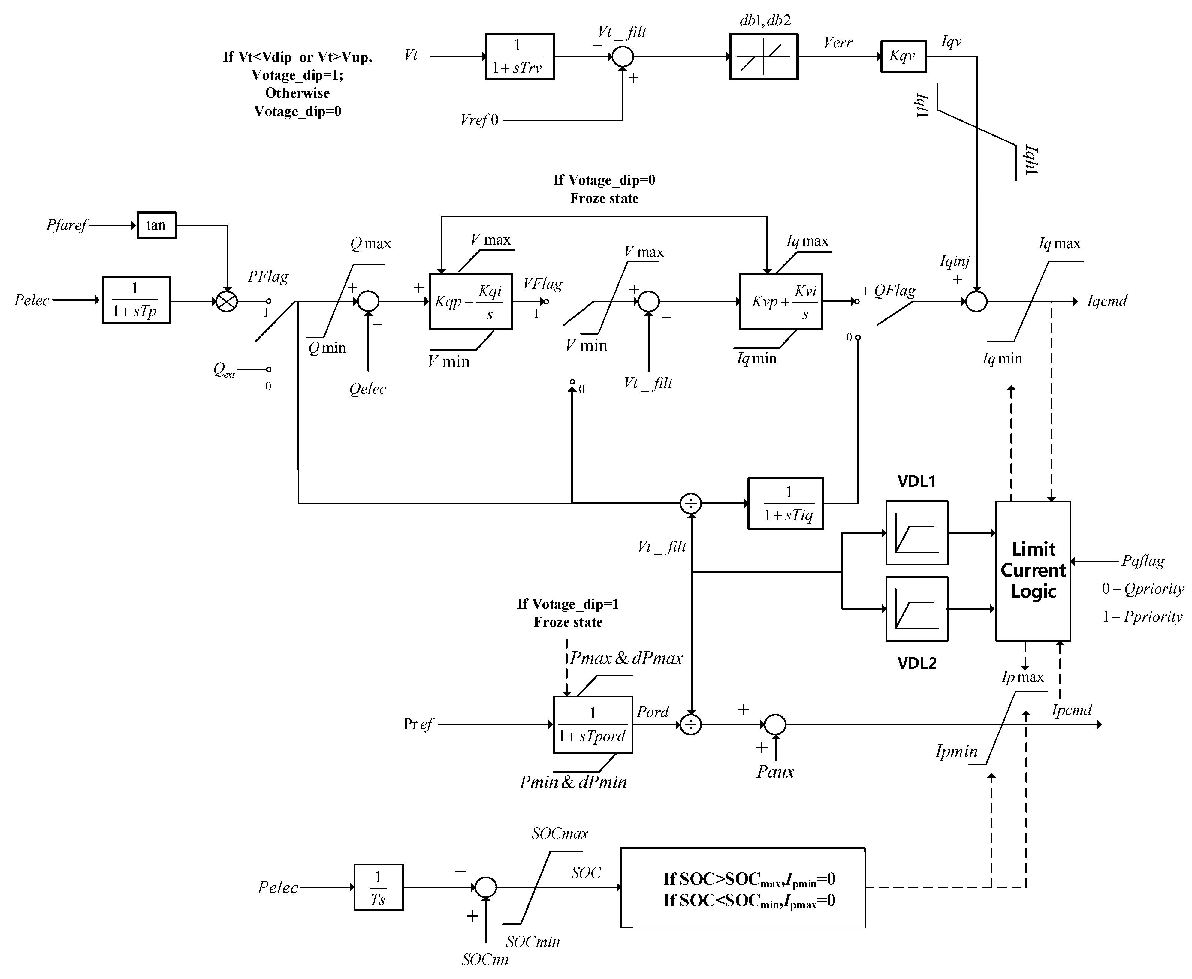
The control strategy of the electrical control part in the energy storage model, as shown in Figure 6.

As shown in Figure 7, the electrical control part of the energy storage model manages the active power and reactive power output, and achieves the aforementioned management by tuning the reference values of active current and reactive current. The reactive power control mode of the energy storage system can switch between different control modes based on the selection of several flags. These modes are shown as follows:

(1)

Local Constant Reactive Power Control: PFlag = 0, QFlag = 0, and VFlag = 0 or 1;

(2)

Local Constant power factor angle control: PFlag = 1, QFlag = 0, and VFlag = 0 or 1;

(3)

Local Node Voltage Control: PFlag = 0, VFlag = 0, and QFlag = 1;

(4)

Local Reactive Power-Voltage Coordinated Control: Pflag = 0, Vflag = 1 and Qflag = 1.

The electrical control part of the energy storage system manages the state of charge (SOC) and controls the maximum output current by constraining upper and lower limits on the reference values for both active and reactive current outputs. Based on the initial state of charge (SOC_ini), the current state of charge of the energy storage system is calculated through the integration of the output active power. During charging, when the energy storage system generates negative active power (P_elec), the SOC tends to increase. Upon reaching the upper limit of the state of charge (SOC_max), the energy storage system needs to restrict charging to prevent battery damage. At this point, Ipmin is set to 0, and the energy storage system can only engage in discharging. During discharging, when the energy storage system outputs positive active power (P_elec), the state of charge tends to decrease. Upon reaching the lower limit of the state of charge (SOC_min), the energy storage system needs to restrict discharging to prevent battery over-discharge damage. At this point, Ipmax is set to 0, and the energy storage system can only engage in charging. The meanings of the variables in Figure 7 are demonstrated in

Table A2. The meaning of variables for energy storage model.

Variable	Description
$V_{dip}$	Activation Logic for Reactive Current Injection at Low Voltage Threshold
$V_{up}$	Activation Logic for Reactive Current Injection at High Voltage Threshold
$Trv$	Voltage Filtering Time Constant (seconds)
$dbd1$	Lower Threshold for Voltage Error Deadband
$dbd2$	Upper Threshold for Voltage Error Deadband
$Kqv$	Reactive Current Injection Gain under Overvoltage and Undervoltage Conditions
$Iqh1$	Reactive Current Injection Upper Limit
$Iql1$	Reactive Current Injection Lower Limit
$V_{ref0}$	User-defined reference (if set to 0, the model initializes it to the initial terminal voltage)
$T_p$	Time constant of the input power filter
$Q_{\max }$	Upper limit of the reactive power regulator
$Q_{\min }$	Lower limit of the reactive power regulator
$V_{\max }$	Upper limit of voltage control
$V_{\min }$	Lower limit of voltage control
$K_{qp}$	Proportional gain of the reactive power regulator
$K_{qi}$	Integral gain of the reactive power regulator
$K_{vp}$	Proportional gain of the voltage regulator
$K_{vi}$	Integral gain of the voltage regulator
$T_{iq}$	Time constant of reactive power regulator
$d{P}_{\max }$	(>0) Maximum rate of change for power reference
$d{P}_{\min }$	(<0) Minimum rate of change for power reference
$P_{\max }$	Maximum power limit
$P_{\min }$	Minimum power limit
$T_{pord}$	Power filter time constant
$V_{q1}$	Voltage 1 in the reactive V-I curve
$I_{q1}$	Current 1 in the reactive V-I curve
$V_{q2}$	Voltage 2 in the reactive V-I curve
$I_{q2}$	Current 2 in the reactive V-I curve
$V_{q3}$	Voltage 3 in the reactive V-I curve
$I_{q3}$	Current 3 in the reactive V-I curve
$V_{q4}$	Voltage 4 in the reactive V-I curve
$I_{q4}$	Current 4 in the reactive V-I curve
$V_{p1}$	Voltage 1 in the active V-I curve
$I_{p1}$	Current 1 in the active V-I curve
$V_{p2}$	Voltage 2 in the active V-I curve
$I_{p2}$	Current 2 in the active V-I curve
$V_{p3}$	Voltage 3 in the active V-I curve
$I_{p3}$	Current 3 in the active V-I curve
$V_{p4}$	Voltage 4 in the active V-I curve
$I_{p4}$	Current 4 in the active V-I curve
$I_{p\max }$	Upper limit of active power
$I_{p\min }$	Lower limit of active power
$I_{q\max }$	Upper limit of reactive power
$I_{q\min }$	Lower limit of reactive power
$SO{C}_{ini}$	Initial state of charge
$SO{C}_{\max }$	Maximum allowable state of charge
$SO{C}_{\min }$	Minimum allowable state of charge
$V_{ref0}$	Bus reference voltage
$P_{faref}$	Power factor reference angle (rad)
$I_{pcmd}$	Active current command value
$I_{qcmd}$	Reactive current command value
$P_{aux}$	Auxiliary input power
$PFlag$	1: Power factor control 0: Reactive power control
$VFlag$	1: Reactive power control 0: Voltage control
$QFlag$	1: Voltage or reactive power control 0: Constant power factor angle or reactive power control
$Pqflag$	0: Reactive power priority 1: Active power priority
$E_n$	Rated battery capacity
$EtaC$	Charging efficiency
$EtaD$	Discharge efficiency

at Appendix A.

Furthermore, the current limiting components (VDL1, VDL2) of the energy storage model are depicted in Figure 7.

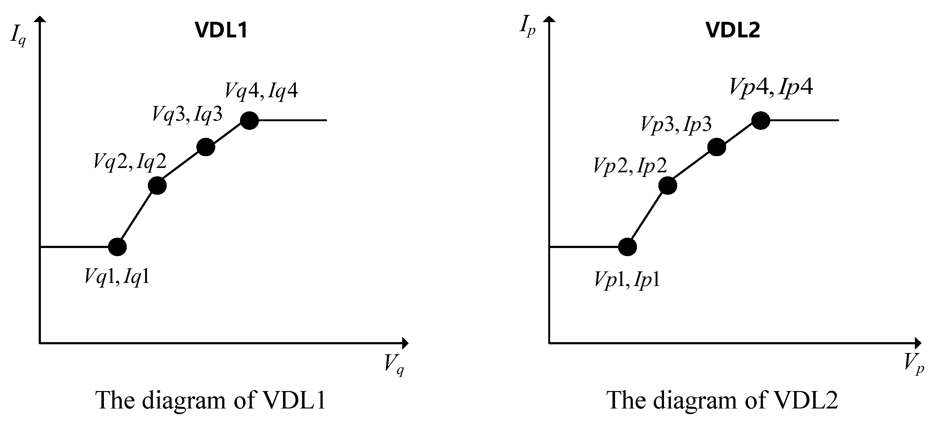
In Figure 8, VDL1 represents the reactive current limiting module for energy storage, while VDL2 denotes the active current limiting module for energy storage. VDL1 generates a corresponding reactive current limit value (I_q) based on the voltage at the PCC of the energy storage device (V_q) and transfers it to the current limiting logic section. Similarly, VDL2 generates an appropriate active current limit value (I_d) based on the voltage at the PCC of the energy storage device (V_d) and passes it to the current limiting logic section (see Figure 7). Since the energy storage device is connected to the distribution network through an inverter, the inverter requires a current protection function. Thus, both reactive and active current outputs have certain limits; the upper limit for reactive current is set as I_q4 in VDL1, and the upper limit for active current is set as I_p4 in VDL2.

In Figure 9, the control strategy of the current converter part of the energy storage model is as follows:

As depicted in Figure 9, the current converter receives active current commands (I_pcmd) and reactive current commands (I_qcmd) from the electrical control part. It interacts with the distribution grid to achieve the exchange of active current (I_p) and reactive current (I_q) through the high-voltage reactive current management section and the low-voltage active current management section. The meanings of the variables in Figure 9 are as shown in

Table A3. The meanings of the variables in Figure 9.

Varaible	Description
$T_g$	Inverter time constant
$I_{pcmd}$	Active current command value
$I_{qcmd}$	Reactive current command value
$rrpwr$	Rate-of-change limit of low-voltage power logic (LVPL)
$Brkpt$	LVPL characteristic voltage 2
$Zerox$	LVPL characteristic voltage 1
$Lvpl1$	LVPL gain
$V_{o\lim }$	Voltage limit of high-voltage reactive current management
$Lypnt1$	High-voltage point of low-voltage active current management
$Lypnt0$	Low-voltage point of low-voltage active current management
$T_{fltr}$	Time constant of the voltage filter used for low-voltage active current management
$K_{hv}$	Overvoltage compensation gain used for high-voltage reactive current management
$I_{q\max }$	Upper limit of the rate of change of reactive current
$I_{q\min }$	Lower limit of the rate of change of reactive current
$Q_{gen0}$	Initial reactive power from load flow calculation
$V_t$	Voltage at the PCC
$Lvplsw$	0: LVPL not enabled 1: LVPL enabled

at Appendix A.

The control strategy of Figure 9 is expressed as follows:

$$I_{qgrid}=I_q-K_{hv}(V_t-V_{o\lim })$$

(7)

$$I_{pgrid}=\left\{\begin{array}{ll}0\hfill & V_t<Lypnt0\hfill \\ I_p\frac{V_t-Lypnt0}{Lypnt1-Lypnt0}\hfill & Lypnt0\le V_t\le Lypnt1\hfill \\ I_p\hfill & V_t>Lypnt1\hfill \end{array}\right.$$

(8)

$$\frac{d{I}_q}{dt}=-\frac{1}{T_g}(I_q+I_{qcmd})$$

(9)

$$\frac{d{I}_p}{dt}=\frac{1}{T_g}(I_{pcmd}-I_p)$$

(10)

$$LVPL=\left\{\begin{array}{ll}0\hfill & V<Zerox\hfill \\ \frac{V-Zerox}{Brkpt-Zerox}\hfill & Zerox\le V\le Brkpt\hfill \\ \infty \hfill & V>Brkpt\hfill \end{array}\right.$$

(11)

$$\frac{dV}{dt}=\frac{1}{T_{fltr}}(V_t-V)$$

(12)

The interaction of reactive current (I_qgird) between the energy storage model’s current converter and the distribution grid is derived from Formula (7). In instances where the PCC voltage is observed to be high, it is advisable to diminish the reactive current input to prevent an increase in grid voltage. Similarly, the active current (I_pgrid) interaction is computed using Formula (8). A lower-than-normal grid connection voltage necessitates a decrease in active current injection, redirecting a greater portion of the output towards reactive current to bolster the grid voltage. Formula (11) outlines the low voltage ride-through (LVRT) control strategy of the energy storage system. If the PCC voltage is detected to be below the standard level, the Lvplsw indicator decides on the activation of LVRT control. This control strategy constricts the active current, ensuring the energy storage system can supply adequate reactive current throughout the LVRT event to maintain grid voltage support.

2.3. Wind Turbine Model

As environmental conservation becomes a growing priority, the allure of new, clean, and efficient energy sources is on the rise. Wind power, in particular, has emerged as a pivotal component in the new energy landscape due to its relatively short development cycle—often spanning just weeks or months—which has propelled its swift expansion. Globally, wind power’s installed capacity has seen an impressive average annual growth rate of 31%, with certain countries achieving even more remarkable increases of up to 60% annually. China, with its vast wind resources, is well-positioned to fulfill its escalating electrical needs through wind energy. Especially in China’s western regions, characterized by abundant wind resources, sparse populations, and dispersed residential areas, the traditional large-scale power grid falls short of meeting electricity demands efficiently. In these areas, localized wind power generation emerges as a viable and effective solution.

To encapsulate, stepping up the exploration and harnessing of wind resources not only promises to mitigate energy deficits but also to refine the prevailing energy mix, which is heavily reliant on coal, oil, and natural gas. This strategy plays a significant role in environmental preservation, curtails energy consumption, and helps temper the global warming crisis by reducing greenhouse gas emissions. Thanks to the ongoing advancement of wind power technologies, tapping into wind resources stands to deliver substantial economic and societal advantages, heralding a bright future for the market.

In this context, the modeling and dynamic simulation of wind turbines emerge as essential components in the exploitation of wind resources. Developing detailed and universally applicable models for wind turbines facilitates their dynamic integration simulations within the distribution grid. This approach not only guides the capacity planning for wind turbine connections to the grid but also supports simulations under fault conditions, assists in crafting and fine-tuning LVRT strategies, and examines the complex dynamics when multiple wind turbines are interconnected with the distribution network.

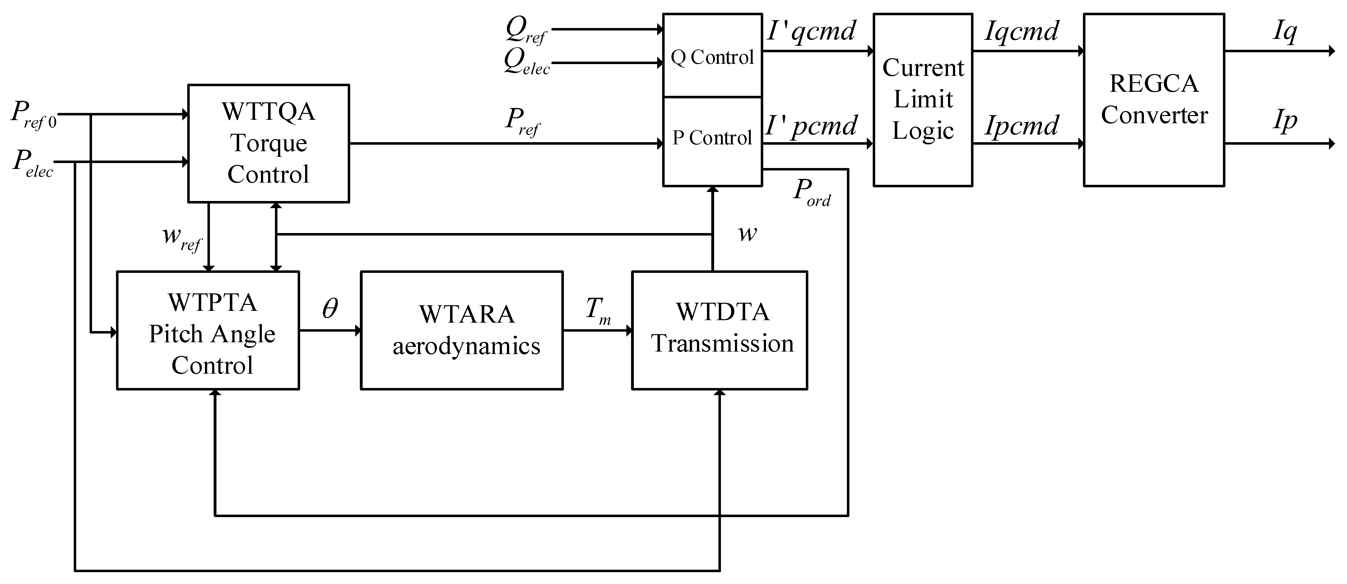
The wind turbine model established in this paper includes modules for torque control, pitch angle control, aerodynamics, transmission, electrical control, and converters (as shown in Figure 10). It is capable of effectively simulating the physical dynamics and electrical behaviors of wind turbines within large-scale simulations of the distribution grid, facilitating dynamic analysis of wind turbine grid integration.

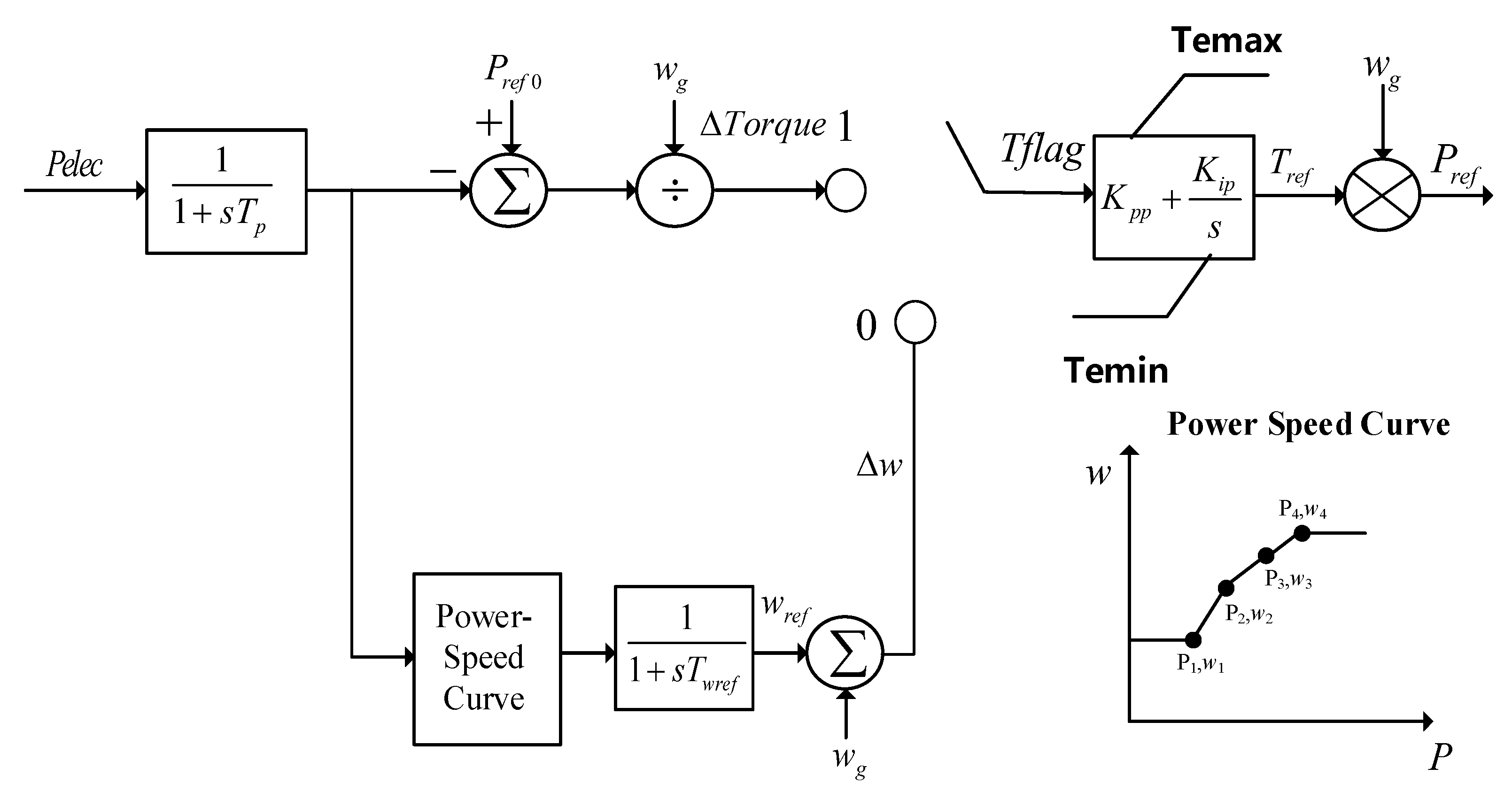
The control strategy of the torque control module in Figure 11 is as follows:

The wind turbine torque control module plays a crucial role in optimizing the efficiency of wind energy conversion. It adjusts the torque applied to the turbine’s rotor to match the wind speed, thereby maximizing power output while minimizing mechanical stress on the turbine. This control module ensures that the turbine operates within its safe operational limits, protecting it from damage caused by excessive wind speeds. By precisely controlling the rotor torque, the module also helps in stabilizing the power generation process, contributing to the reliability and stability of the power grid to which the wind turbine is connected. The torque control module receives data on the active power output (P_elec), the initial active power reference (P_ref0), and the rotational speed (w_g) of the wind turbine. And the torque control module outputs the active power reference (P_ref) to the wind turbine’s electrical control module and the reference for rotational speed (w_ref) to the wind turbine’s pitch angle control module, facilitating dynamic torque control of the wind turbine. The power–speed curve dynamically adjusts the rotational speed based on the measured power data. For instance, when the measured power is P₃, the rotational speed is set to w₃, ensuring optimal efficiency and performance.

Some mathematical relationships for the variables are expressed as follows:

$$P_{ref}=K_{pp}(w_g-w_{ref})+P_{ref2}$$

(13)

$$\frac{d{P}_{ref2}}{dt}=\left\{\begin{array}{cc}{K}_{ip}(w_g-w_{ref})\hfill & Voltage\_dip=0\hfill \\ 0\hfill & Voltage\_dip=1\hfill \end{array}\right.$$

(14)

$$\frac{d{w}_{ref}}{dt}=\frac{1}{T_{wref}}(f(P)-w_{ref})$$

(15)

In Formula (14), Voltage_dip is determined by the electrical control module of the wind turbine generator. I_t is set to 1 when the voltage of the wind turbine at the PCC falls below a lower limit or exceeds an upper limit (V_t < V_dip or V_t > V_up); otherwise, it is set to 0.

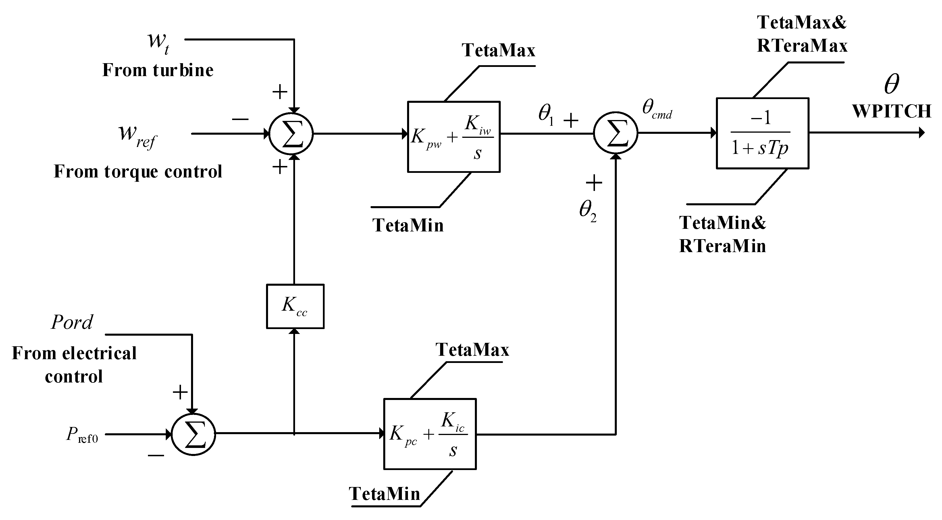
The control strategy of the pitch angle control module in Figure 12 is as shown in the following diagram:

The pitch angle control module for wind turbines plays a pivotal role in managing the angle of the blades relative to the wind. By adjusting the pitch angle, this module regulates the amount of wind energy captured by the turbine. In low wind conditions, it decreases the pitch angle to capture as much wind as possible, maximizing power generation. Conversely, in high wind conditions, it increases the pitch angle to reduce the wind force on the blades, preventing overloading and potential damage to the turbine. This control strategy not only optimizes the efficiency of power generation across varying wind speeds but also enhances the longevity and reliability of the wind turbine system. The pitch angle control module receives the initial reference value for active power (P_ref0), rotational speed information from the turbine (w_t), the reference speed information from the torque control module (w_ref), and the power command (P_ord) from the electrical control module. It outputs the pitch angle information (θ) to the wind turbine’s aerodynamics module.

Some mathematical relationships for the variables are expressed as follows:

$$\frac{d\theta }{dt}=\frac{1}{T_p}({\theta }_1+{\theta }_2-\theta )$$

(16)

$${\theta }_1=K_{pw}(w_t-w_{ref}+K_{cc}{P}_{ord}-K_{cc}{P}_{ref})+{\theta }_{12}$$

(17)

$${\theta }_2=K_{pc}(P_{ord}-P_{ref})+{\theta }_{22}$$

(18)

$$\frac{d{\theta }_{12}}{dt}=K_{iw}(w_t-w_{ref}+K_{cc}{P}_{ord}-K_{cc}{P}_{ref})$$

(19)

$$\frac{d{\theta }_{22}}{dt}=K_{ic}(P_{ord}-P_{ref})$$

(20)

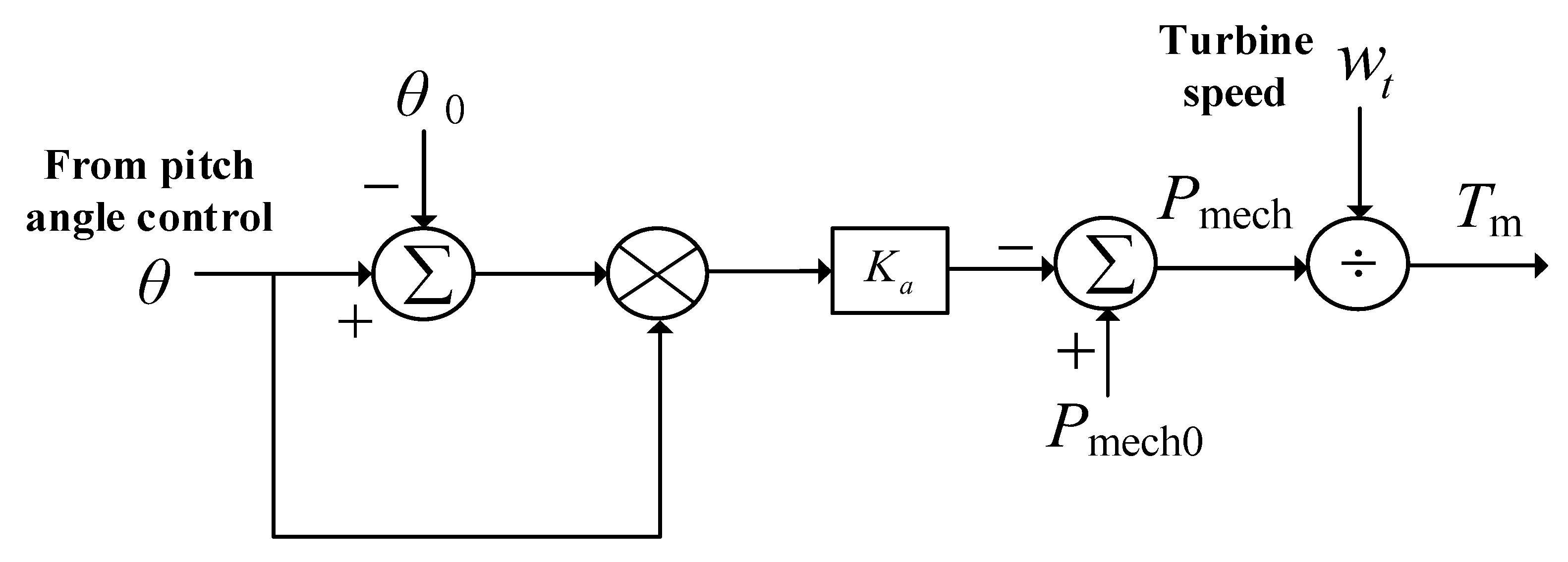
The control strategy of the aerodynamics module in Figure 13 is as shown in the following diagram:

The aerodynamics module of a wind turbine is critical for analyzing and optimizing the interaction between the wind and the turbine blades. This module computes the lift and drag forces exerted by the wind on the blades, which are essential for determining the turbine’s power output. By understanding these aerodynamic forces, the module helps in designing blades that maximize efficiency by extracting the maximum amount of energy from the wind while minimizing losses due to drag. Additionally, the aerodynamics module plays a vital role in predicting the performance of the turbine under various wind conditions, enabling more accurate forecasting of energy production. The aforementioned functions can be achieved by flexibly adjusting the parameter K_a (the aerodynamics gain factor). The aerodynamics module receives pitch angle information (θ) from the pitch angle control module, initial mechanical power information (P_mech0), turbine speed information (w_t), and initial pitch angle information (θ₀). The aerodynamics module outputs torque information (T_m) to the transmission module of the wind turbine. Some mathematical relationships for the variables are expressed as follows:

$$P_{mech}=P_{mech0}-K_a\theta (\theta -{\theta }_0)$$

(21)

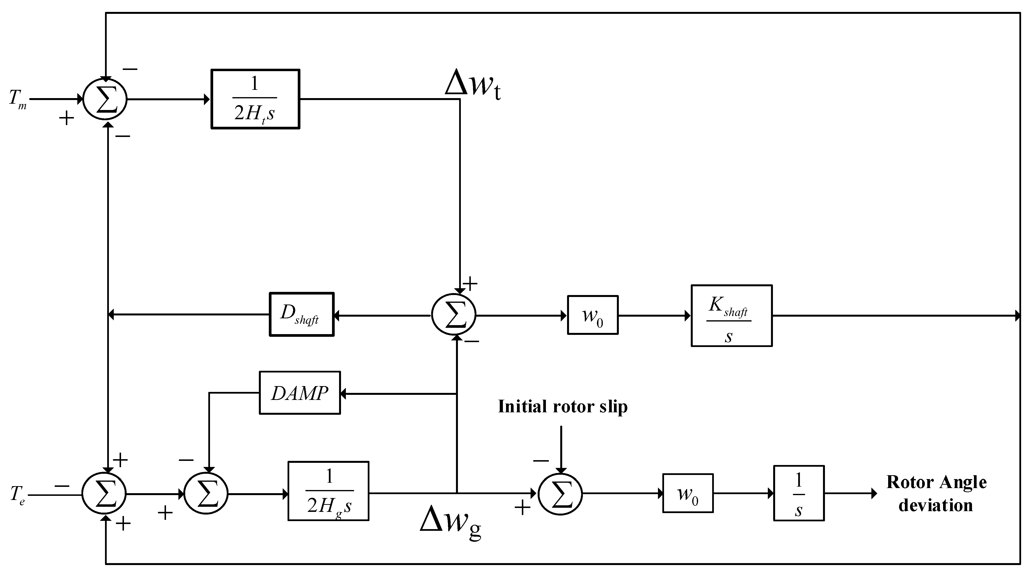
The control strategy of the transmission module in Figure 14 is as follows:

The Generic Drive Train Model for wind turbines serves as a fundamental tool for simulating the mechanical and electrical interactions within the turbine’s drive train system. This model encapsulates the dynamics between the turbine’s rotor, gearbox, and generator, offering insights into how kinetic energy from the wind is converted into electrical energy. The transmission module receives torque information (T_m) from the aerodynamics module, and outputs speed information (w) to the electrical control module. Some mathematical relationships for the variables are expressed as follows:

$$\frac{d\Delta w_g}{dt}=\frac{1}{2H_g}(-\frac{P_{gen}}{w_g}+K_{shaft}{\delta }_{tg}+D_{shaft}(\Delta w_t-\Delta w_g))$$

(22)

$$\frac{d\Delta w_t}{dt}=\frac{1}{2H_t}(\frac{P_{mech}}{w_t}-K_{shaft}{\delta }_{tg}-D_{shaft}(\Delta w_t-\Delta w_g))$$

(23)

$$w_g=w_0+\Delta w_g$$

(24)

$$w_t=w_0+\Delta w_t$$

(25)

$$\frac{d{\delta }_{tg}}{dt}=\Delta w_t-\Delta w_g$$

(26)

In Equation (26), the variable “δ_tg” represents an intermediate variable in the process “(Δw_t − Δw_g)/s”.

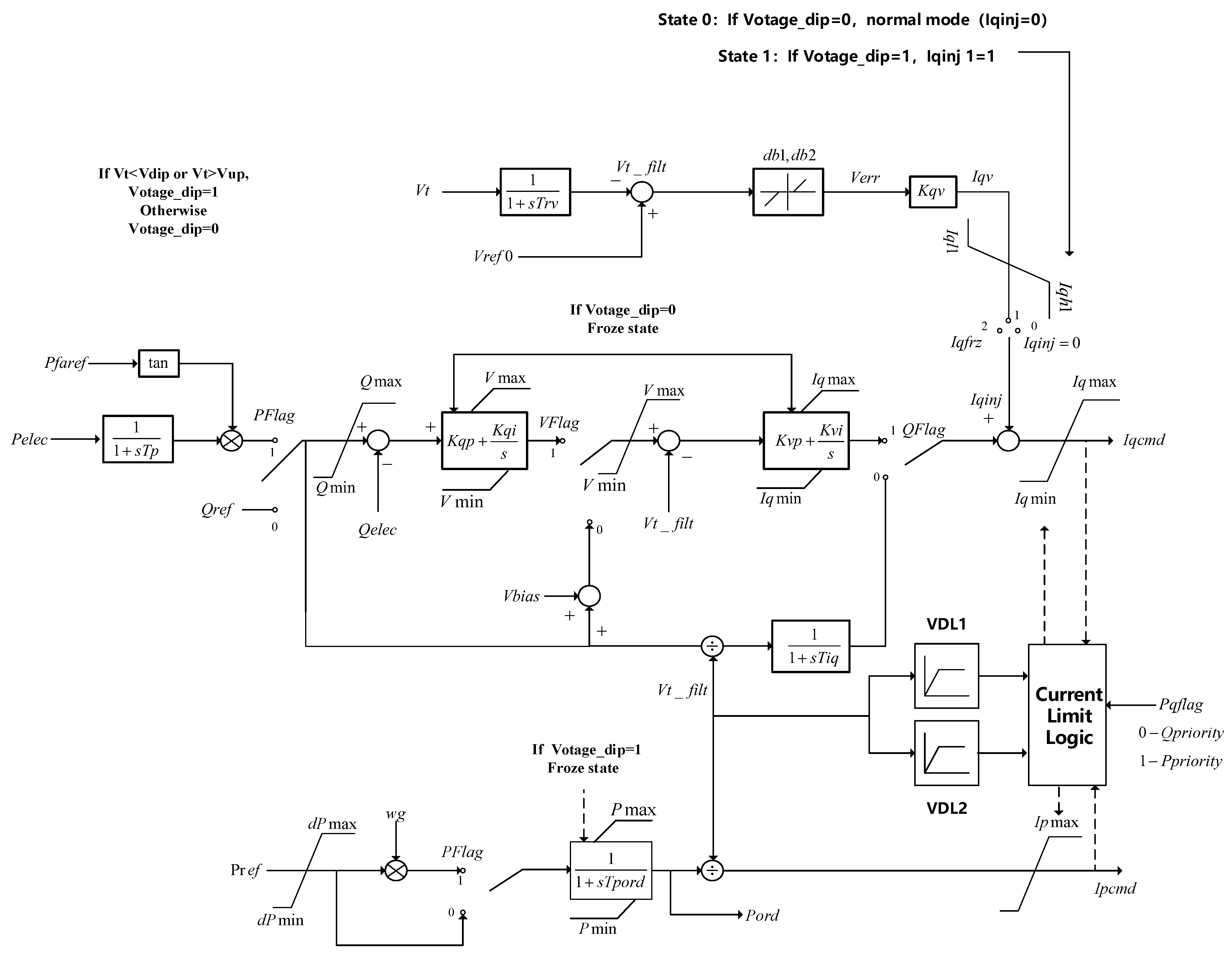
The control strategy of the electrical control module in Figure 15 is as follows:

The electrical control module of a wind turbine plays a critical role in managing the electrical aspects of power generation. This module oversees the conversion of mechanical energy from the wind turbine into electrical energy that is compatible with the power grid. It regulates the voltage and frequency of the electricity generated to ensure it meets grid requirements. Additionally, the module optimizes the power output in response to varying wind conditions by adjusting the output current reference values (I_qcmd and I_pcmd). It also provides protective functions to safeguard the turbine’s electrical components from faults, overloads, and other potentially damaging conditions. By precisely controlling the electrical parameters, the module enhances the efficiency, reliability, and grid compatibility of the wind turbine’s power generation. The electrical control module receives active power reference value information (P_ref) from the torque control module, wind turbine generator speed information (w) from the transmission module, reactive power reference value information (Q_ref), and measured the reactive power information (Q_elec) and active power information (P_elect) that wind turbine outputs. The electrical control module outputs active power command (P_ord) to the pitch angle control module, and active current reference value command (I_pcmd) and reactive current reference value command (I_qcmd) to the inverter module. To ensure the protection of the wind turbine model, these current reference values are regulated by the current limit logic. This logic also accounts for voltage management under fault conditions, as detailed in Section 2.2 with the descriptions of VDL1 and VDL2. The electrical control module facilitates different control modes, such as local constant reactive power control, local constant power factor angle control, local node voltage control, and local reactive power-voltage coordinated control. These modes are activated through the toggling of various flags, with comprehensive details provided in Section 2.2.

Some mathematical relationships for the variables are expressed as follows:

$$Voltage\_dip=\left\{\begin{array}{cc}0\hfill & V_{up}\ge V_t\ge V_{dip}\hfill \\ 1\hfill & Others\hfill \end{array}\right.$$

(27)

$$I_{qinj}=\left\{\begin{array}{ll}0\hfill & Voltage\_dip=0\hfill \\ K_{qv}(V_{ref}-V_{tfilt})\hfill & Voltage\_dip=1\hfill \end{array}\right.$$

(28)

$$I_{qcmd}=I_{qord}+I_{qinj}$$

(29)

$$I_{pcmd}=\frac{P_{ord}}{V_{tfilt}}$$

(30)

$$\frac{d{V}_{tfilt}}{dt}=\frac{1}{T_{rv}}(V_t-V_{tfilt})$$

(31)

$$\frac{d{I}_{qord}}{dt}=\left\{\begin{array}{ll}\frac{1}{T_{iq}}(\frac{Q_{ext}}{V_{tfilt}}-I_{qord})\hfill & Voltage\_dip=0\hfill \\ 0\hfill & Voltage\_dip=1\hfill \end{array}\right.$$

(32)

$$\frac{d{P}_{ord}}{dt}=\left\{\begin{array}{ll}\frac{1}{T_{pord}}(w_g{P}_{ref}-P_{ord})\hfill & Voltage\_dip=0\hfill \\ 0\hfill & Voltage\_dip=1\hfill \end{array}\right.$$

(33)

$$I_{q\max }=\min \left\{VDL1,\left.I_{r\max }\right\}\right.$$

(34)

$$I_{p\max }=\min \left\{VDL2,\left.\sqrt{{i^2}_{r\max }-{i^2}_{qcmd}}\right\}\right.$$

(35)

The inverter module has been introduced in the energy storage model and will not be reiterated here.

2.4. Electric Vehicle Model

In the wake of V2G technology’s advancement and deployment, electric vehicles (EVs) have rapidly evolved into a burgeoning, controllable resource on the demand side, characterized by their interruptibility and adjustability. Their incorporation into grid regulation is marked by rapid responsiveness and remarkable cost-effectiveness. Nonetheless, integrating EVs into the grid and involving them in grid management could potentially disrupt the distribution network, posing risks to its operational safety and stability. By developing a model that simulates the dynamics of EV participation in grid regulation, the capability for large-scale integration of EVs into grid adjustments is thoroughly examined. This exploration aids in crafting control strategies for EV involvement in voltage support and frequency management amidst the extensive introduction of renewable energies, aiming to bolster voltage and frequency stability, as well as enhance the distribution grid’s resilience to and recovery from faults, thereby elevating consumer satisfaction with electricity services.

The EV model proposed in this study employs a PQ grid connection control strategy to manage both the active and reactive power outputs of EVs, alongside simulating SOC management and battery protection mechanisms. Additionally, it introduces a control strategy enabling EVs to participate in voltage and frequency stabilization within the distribution grid, facilitating a seamless integration of EV charging and discharging activities with the grid’s dynamic demands. This model provides a foundational reference for the inclusion of electric vehicles in the distribution network’s regulatory framework, presenting an innovative approach to harmonizing grid operations with EV control.

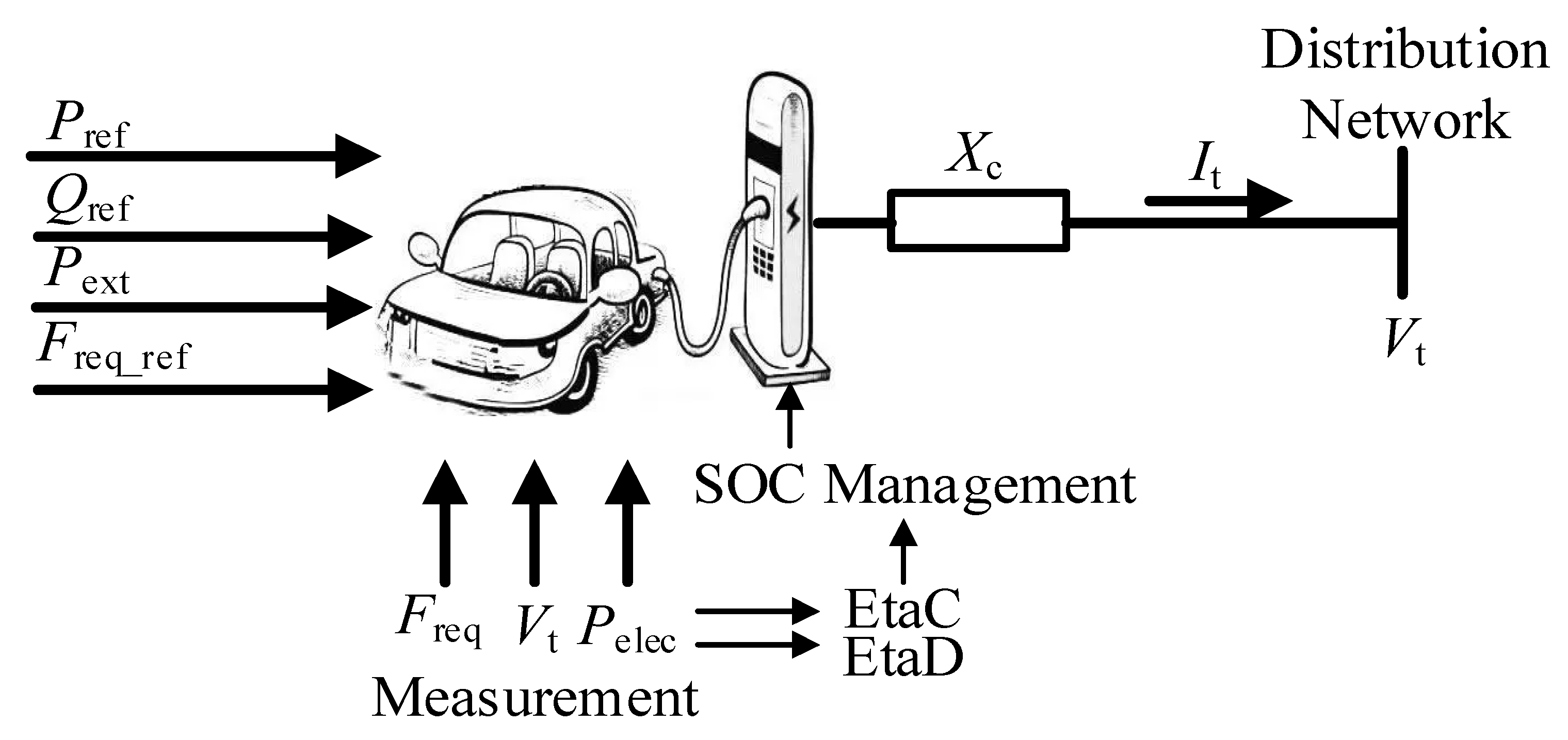
The EV model showcased in this research, as illustrated in Figure 16, processes inputs such as active (P_ref) and reactive (Q_ref) power reference values, an additional external power input (P_ext), and a frequency reference (F_{req_ref}). It measures the frequency (F_req) and voltage (V_t) at the EV charging station’s point of grid connection, alongside the active power (P_elec) exchange with the distribution grid. This active power, combined with information on charging (EtaC) and discharging efficiencies (EtaD), forms the foundation of the model’s SOC management system. Equipped for detailed power management, SOC regulation, and participation in voltage and frequency regulation at the PCC, this model emerges as an integral resource for bolstering grid reliability and enhancing the operational efficiency of electric vehicles.

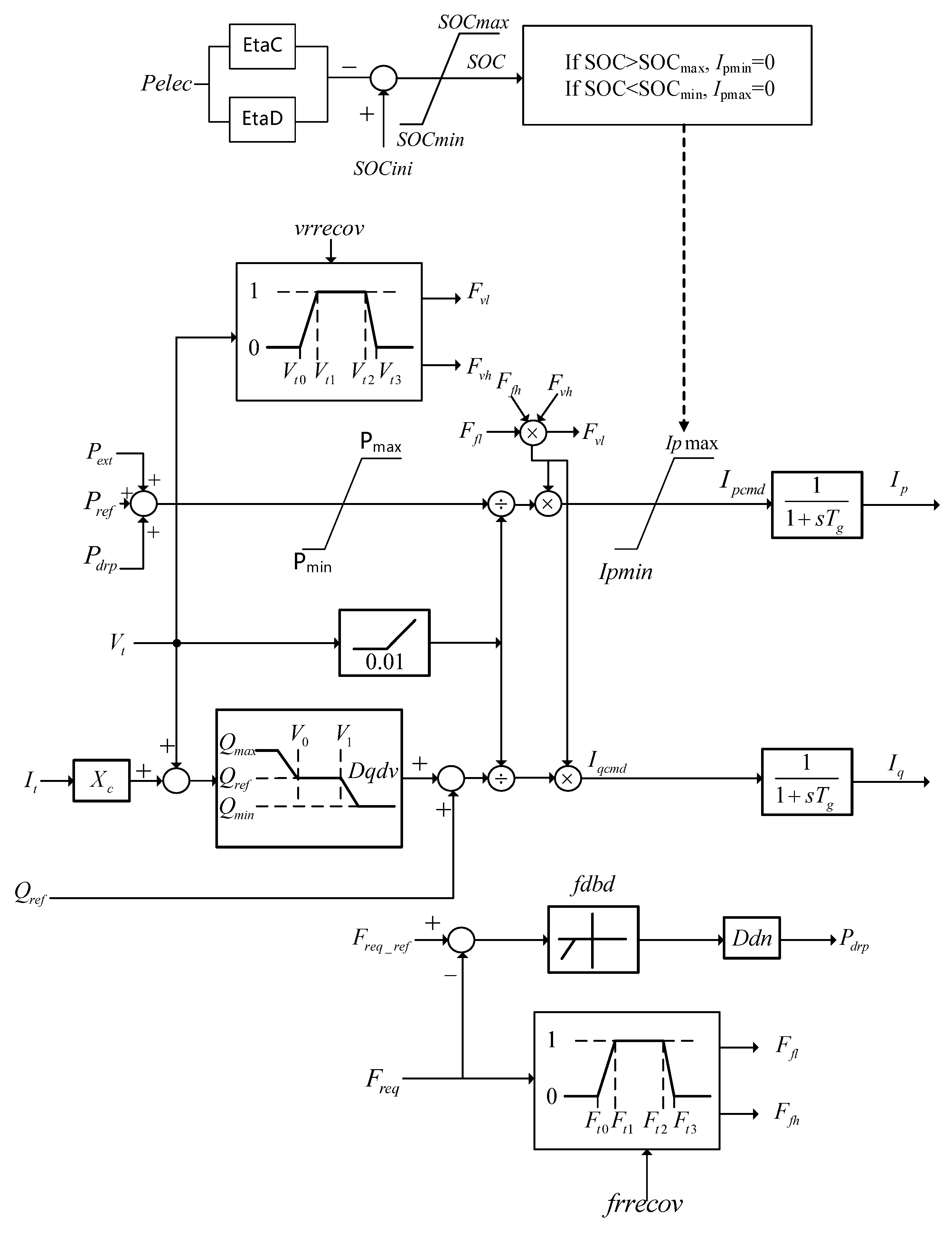
The control strategy of the electric vehicle model constructed in this paper is shown in the following Figure 17:

The components concerning power management, engagement in voltage regulation of the distribution grid, and participation in frequency management of the grid mirror those established in the distributed photovoltaic model, and thus, will not be redundantly detailed here. As for the SOC management, the control strategy is defined as follows:

$$\left\{\begin{array}{cc}SOC=SO{C}_{ini}-P_{elec}\times EtaC\hfill & Ch\arg e state\hfill \\ SOC=SO{C}_{ini}-P_{elec}\times EtaD\hfill & Disch\arg e state\hfill \end{array}\right.$$

(36)

$$\left\{\begin{array}{ll}{I}_{p\min }=0\hfill & SOC>SO{C}_{\max }\hfill \\ I_{p\max }=0\hfill & SOC<SO{C}_{\min }\hfill \end{array}\right.$$

(37)

The calculation of the SOC for EVs during their charging and discharging phases is delineated in Formula (36), with SOC_ini denoting the EV’s initial SOC. When an EV is being charged, Pelec is assumed to be negative, which causes the SOC to rise. In contrast, when the EV is discharging, Pelec becomes positive, leading to a reduction in the SOC. Should the SOC surpass the designated maximum limit (SOC_max), the minimum threshold for the active current reference (I_pmin) is adjusted to zero, restricting the active current to only positive values and thereby halting further charging while permitting discharging. On the other hand, if the SOC drops below the minimum permissible limit (SOC_min), the maximum threshold for the active current reference (I_pmax) is reduced to zero, limiting the active current to negative values only, thus precluding further discharge and enabling charging. This regulatory strategy ensures the SOC of the EV remains within an acceptable range (SOC_min < SOC < SOC_max), effectively preventing the battery from being overcharged or over-discharged.

3. Case Studies

The key equipment models for the distribution network developed in this study have been incorporated into our team’s proprietary distribution network automation simulation platform, WHU-Dis. Engineered on Python 3.9, this platform is distinguished by its remarkable extensibility and superior capabilities for external interactions. The simulations are conducted on a personal computer outfitted with a 2.9 GHz i5 processor and 16 GB of RAM, which is located in Wuhan, China. Within the WHU-Dis environment, the IEEE-33 node distribution network topology has been implemented. This platform enables integration and dynamic simulation of the developed models for distributed photovoltaic, energy storage, wind turbine, and electric vehicle, effectively validating the effectiveness of the proposed modeling approaches.

3.1. Simulation of Distributed PV

Figure 18 illustrates the IEEE-33 node topology, showcasing the incorporation of distributed PV systems at Buses 11, 19, 23, and 26, with each node connecting ten distributed PV units. A three-phase short circuit fault is orchestrated at Bus 31, commencing at 2.5 s and concluding by 2.7 s. The comprehensive simulation covers a duration of 5 s and employing a timestep of 0.0001 s.

Figure 19 and Figure 20 respectively showcase the active and reactive power outputs of the first distributed PV units connected at buses 11, 19, 23, and 26. The capacity of a distributed PV unit is 0.4 MW. Figure 21 presents the dynamic voltage at these nodes, while Figure 22 reveals the frequency of the first distributed PV units connected at those nodes. The occurrence of a three-phase short circuit at bus 31 notably impacts the distributed PV installations at bus 11 and bus 26, leading to significant voltage drop as highlighted in Figure 21. These pronounced voltage declines at the mentioned nodes trigger a decrease in the output power of the associated distributed PV units during the event, as demonstrated in Figure 19 and Figure 20. The active and reactive power outputs of PVD1_1 and PVD1_4 undergo a downturn during the fault event, with all distributed PV units progressively reverting to their predefined outputs post-fault clearance.

3.2. Simulation of Energy Storage Model

Figure 23 presents the IEEE-33 node topology, featuring the energy storage model interconnected at buses 13, 19, 23, and 26. The capacity of an energy storage unit is 0.4 MW. A three-phase short circuit fault is introduced at bus 25, initiating at 2 s and resolved by 2.3 s. The entire simulation extends over a period of 5 s, utilizing a detailed simulation timestep of 0.0001 s.

Figure 24 showcases the active power output from energy storage units connected at buses 13, 19, 23, and 26. Figure 25 showcases the reactive power output from energy storage units connected at buses 13, 19, 23, and 26. Dynamic voltage variations at these locations are depicted in Figure 26, while Figure 27 reveals the progression of the SOC for the four energy storage systems. The occurrence of a three-phase short circuit at bus 25 significantly impacts the energy storage system at bus 23, causing a notable voltage drop at this node, as emphasized in Figure 26. During the fault event, all energy storage units were in the charging mode and experienced a decrease in charging power. Once the fault was cleared, the charging power began to recuperate, ultimately returning to its pre-fault level, as illustrated in Figure 24. Initially set at 0.4, the SOC for each of the four energy storage units began their charging cycle. The units connected to buses 13 and 19 exhibited a higher charging rate compared to the more gradual pace of the unit at bus 23. Throughout the charging process, all units experienced a steady increase in SOC. However, the increase in SOC for the units at bus 13 and bus 19 was more pronounced, outpacing the more modest rate of increase at bus 23, as demonstrated in Figure 27.

3.3. Simulation of Wind Turbine Model

Figure 28 displays the IEEE-33 node topology, featuring the integration of the wind turbine model at buses 13, bus 19, bus 23, and bus 26. The capacity of a wind turbine unit is 0.8 MW. A three-phase short circuit fault is introduced at bus 25. This fault is initiated at 2 s and rectified by 2.3 s. The entire simulation spans 5 s, utilizing a detailed simulation timestep of 0.0001 s.

Figure 29 displays the active power output from wind turbines connected at buses 13, bus 19, bus 23, and bus 26, while Figure 30 details their reactive power output. The voltage dynamics at these nodes are captured in Figure 31, and Figure 32 illustrates the variations in rotational speeds for the four wind turbines. The occurrence of a three-phase short circuit at bus 25 significantly affects the wind turbine at bus 23, leading to an obvious voltage drop at this node, as highlighted in Figure 31. On this basis, this wind turbine experiences the most pronounced active power fluctuations during the fault event, as depicted in Figure 29.

During the fault event, there is a noticeable reduction in the active power output across all wind turbines, which subsequently returns to their initial set values once the fault is rectified. The wind turbine at bus 23 sees a swift drop in active power output during the fault event, resulting in an accelerated increase in its rotational speed—the most rapid among all the turbines, as demonstrated in Figure 32.

3.4. Simulation of EV Model

Figure 33 illustrates the IEEE-33 node topology, incorporating the EV model at buses 9, 13, 19, 23, 26, and 28, with each bus integrating ten EV units. The capacity of an EV units is 0.4 MW. A three-phase short circuit fault is set at bus 16. This fault initiates at 2 s and is resolved by 2.3 s, with the entire simulation spanning 5 s and utilizing a precise simulation timestep of 0.0001 s.

The active power output of the first electric vehicle connected at bus 9, bus 13, bus 19, bus 23, bus 26, and bus 28 is shown in Figure 34, while Figure 35 captures the voltage dynamics at these nodes. Figure 36 presents the SOC progression for these electric vehicles, and Figure 37 reveals the frequency alterations of these electric vehicles. The occurrence of the three-phase fault at bus 16 markedly affects electric vehicles connected at bus 9 and bus 13, evidenced by a significant voltage drop at these nodes. In response to the fault event, the electric vehicles’ charging power diminishes, transitioning from a charging to a discharging phase, thus offering critical support for grid frequency and voltage stabilization during emergencies.

3.5. Simulation of Distributed PV and Energy Storage Model

Figure 38 illustrates the IEEE-33 node topology, showcasing the incorporation of distributed PV models and energy storage models at buses 11, 19, 23, and 26, with each node connecting eight distributed PV units and two energy storage units. The capacity of a distributed PV unit is 0.4 MW, and the capacity of an energy storage unit is 0.25 MW. A three-phase short circuit fault is orchestrated at bus 22, commencing at 1.0 s and concluding by 1.1 s. The comprehensive simulation covers a duration of 5 s and employing a timestep of 0.0001 s.

Figure 39 and Figure 40 respectively showcase the active and reactive power outputs of the first distributed PV units connected at buses 11, 19, 23, and 26. Figure 41 and Figure 42 respectively showcase the active and reactive power outputs of the first energy storage units connected at buses 11, 19, 23, and 26. Figure 43 presents the dynamic voltage at buses 11, 19, 23, and 26, while Figure 44 reveals the frequency of these buses.

The occurrence of a three-phase short circuit at bus 22 notably impacts the distributed PV and energy storage units installed at buses 19, leading to significant voltage drop as highlighted in Figure 43. The pronounced voltage drops at the mentioned bus trigger a fluctuation in the output power of the associated distributed PV units and energy storage units during the event, as demonstrated in Figure 39, Figure 40, Figure 41 and Figure 42. The active power outputs from PVD1_2, which connected to bus 19, exhibits a trend of initially decreasing and then increasing. The energy storage unit connected at bus 19 (ESD1_2), aiming to provide voltage and frequency support, shows a significant increase in active power output during the fault period.

Considering the variability in distributed PV units’ outputs due to weather conditions, it is crucial to explore the voltage and frequency response dynamics of the distribution network under fault scenarios where distributed PVs are incapacitated, leaving energy storage as the primary energy source. This result should be contrasted with situations where distributed PVs are fully operational, providing power, to highlight how network responses vary across different operational states. Specifically, the distributed PV units connected at buses 23 and 26 will be disconnected, and a three-phase short-circuit fault will be introduced at bus 22. This fault will occur at 1.0 s and be cleared at 1.1 s. Figure 45 illustrates the voltage dynamics at the PCC of these distributed units, while Figure 46 details the frequency dynamics at the PCC of these units. It is clearly noticeable that the loss of some distributed PV units’ output leads to increased volatility in the voltage dynamics at nodes 11 and 19, characterized by deeper voltage dips and higher spikes. Likewise, the frequency fluctuations at various PCC are markedly more severe. Yet, once the fault is isolated, voltage and frequency levels steadily revert to their standard operational conditions. This recovery underscores the pivotal role of energy storage in offering crucial voltage and frequency stabilization during the course of the fault dynamics.

3.6. Simulation of Distributed PV Model, Energy Storage Model, and EV Model

Figure 47 illustrates the IEEE-33 bus topology, showcasing the incorporation of distributed PV models, energy storage models, and EV models. The distributed PV units and energy storage units are connected to buses 11, 19, 23, and 26, with each bus connecting eight distributed PV units and two energy storage units. The EV units are connected to bus 30 and bus 32, with each bus connecting ten EV units. The capacity of a distributed PV unit is 0.4 MW, the capacity of an energy storage unit is 0.25 MW, and the capacity of an EV unit is 0.4 MW. A three-phase short circuit fault is orchestrated at bus 22, commencing at 1.0 s and concluding by 1.1 s. The comprehensive simulation covers a duration of 5 s and employing a timestep of 0.0001 s.

Figure 48 and Figure 49 respectively showcase the active and reactive power outputs of the first distributed PV units connected at buses 11, 19 and the first EV units connected at bus 30, 32. Figure 50 presents the voltage dynamics at buses 11, 19, 23, 26, 30 and 32, while Figure 51 reveals the frequency dynamics at these buses. Following a three-phase short circuit fault at bus 22, voltage and frequency fluctuations are observed at the interconnection points of various renewable energy devices, causing variances in the power outputs of both distributed PV units and EV units. The power fluctuations at EV interconnection points are significantly more pronounced compared to those at distributed PV locations. Furthermore, the return to stability for both voltage and frequency at nodes connected to EVs takes a notably longer period post-fault clearance.

4. Conclusions

This paper proposes a data–physics-driven modeling approach for automating simulations in distribution systems. By leveraging a streamlined and uniform framework of linear differential equations featuring adjustable coefficients, it effectively captures the inherent physical properties of various device categories. Detailed models for distributed photovoltaic, wind turbine, energy storage system, and electric vehicle are meticulously discussed. Characterized by their openness, these models facilitate the integration of real-time data to adjust undetermined coefficients, thereby providing an accurate representation of equipment dynamics across different intervals. Constructed on the Python platform, this modeling approach is highly compatible, supporting the requirements for extensive, real-time simulation of the distribution network. Demonstrations of dynamic simulations connected to an IEEE-33 node distribution network substantiate the practicality and efficiency of the proposed methodology.