A Coarsened-Shell-Based Cosserat Model for the Simulation of Hybrid Cables

Abstract

The simulation of elastic slender objects like cables is essential for industrial applications in predicting elastic behaviors and life cycles. The Cosserat model and its variants are the dominant approaches due to their high efficiency and accuracy. However, these assume cables with homogeneous interiors and thus cannot simulate hybrid cables containing different materials. We address this by developing a novel coarsened-shell-based Cosserat (CSC) model. The CSC model constructs a material-aware elastic energy function along the cable’s cross-section to describe the global elastic behavior. The CSC model is specifically developed by carefully leveraging the strengths of three approaches: the Cosserat theory to model slender cables, the Kirchhoff–Love shell theory to model the cable’s cross-sectional energy, and numerical coarsening to reduce the degrees of freedom in the shell simulation via constructing a set of new types of material-aware shape/base functions. This allows the more accurate computation of the local and global deformations of hybrid cables, surpassing the classical Cosserat models in accuracy.

1. Introduction

The mechanical simulation of slender elastic objects, such as long-distance cables or ropes, differs significantly from traditional simulations of 3D bulk models as their length is much greater than their section radius. The Cosserat theory [1,2,3] is a classical and widely adopted model for the efficient simulation of slender cables of high accuracy. It models a slender cable as a centerline with an attached material frame, which together reduces the simulation costs but simultaneously produces realistic elastic deformations such as buckling [2,4]. A more comprehensive review of the Cosserat model is given in [5,6,7].

However, practical industrial cables, as considered in this study, are generally in the form of a hybrid cable that contains different materials or is made up of different types of cables. They can be described as a cable with a heterogeneous interior material distribution, taking the void space as a soft material with a low Young’s modulus. The direct modeling of such hybrid cables as a Cosserat model or one of its variants, however, will reduce the simulation accuracy as the local material frame contained within the Cosserat model does not have enough degrees of freedom (DOFs) to adequately reflect the complex interior deformations. On the other hand, the direct simulation of hybrid cables would be computationally expensive and would not allow for real-time simulation as it requires a dense mesh to fully capture the variations in the material distribution along each part of the interface, thus greatly reducing the simulation speed [8,9]. As a consequence, there is still no satisfactory solution in simulating such slender hybrid cables with heterogeneous material distributions so as to realize simulation speeds that can meet the real-time requirements while guaranteeing the simulation’s accuracy [10].

Related Work

Various approaches have been proposed in modeling and simulating the elasticity of such slender objects as cables—for example, the spring-mass model [11,12], Cosserat elastic rod [13,14], and energy curve method [15,16,17]. Different modeling approaches may correspondingly result in differences in the scope of application. For example, the energy curve method is mainly used in the static simulation of cables, which can only reflect their bending and stretching deformations. The spring-mass model [11,12] is only suitable for the dynamic simulation of elastic slender objects. Due to the simplification of the model, it cannot truly reflect any local deformation of the object. The Cosserat model [5,18] is much improved in this aspect in its good ability to reflect the bending, twisting, shearing, and stretching deformation of a slender object, and it can accurately simulate its posture in three-dimensional space. A compact Cosserat model was recently proposed that further improves the efficiency of cable simulation [19,20].

In the Cosserat theory, the elastic rod is modeled as a continuous 1D curve in 3D space, with an attached orthonormal frame at each point of the curve. The Cosserat theory can be used to simulate hair, ropes, and single cables but is not applicable to some elastic slender objects with complex material distributions, such as woven belts composed of different types of fibers, braided hoses composed of multiple material layers, and medical catheters similar to hybrid cables. However, some research efforts have been devoted to improving the accuracy of the Cosserat model by considering different material distributions [21,22,23].

For example, the Cosserat model has been applied to models of anisotropic materials, such as magnetic filaments [21] or sticky threads [23], by reconstructing the bending stiffness and shear stiffness matrices of the material distribution at the energy-reactive section to reflect the different material distributions of the objects. However, the process of reconstructing the material matrix is not well applied to general cases. Hybrid cables, as studied here, have a much larger number of cable types and thus more complex material distributions. It then becomes very challenging to obtain such a material matrix. We instead construct material-aware shape functions to cope with these challenges.

Li et al. proposed a hybrid model to simulate a hollow tube with a deformable cross-section by binding a surface mesh model to a Cosserat rod, where the Cosserat rod was used to simulate the global bending, torsion, shear, and stretch of the tube, while a surface mesh model was used to represent the surface of the hollow tube [22]. This hybrid method allows the surface to be realistically and effectively deformed according to the shape of the reference rod and the surface elastic energy, thus enabling the simulation of elastic hollow tubes with inhomogeneous materials. However, it cannot be well applied to hybrid cables with complex material distributions.

In order to achieve high-accuracy simulation for hybrid cables consisting of heterogeneous materials, a novel coarsened-shell-based Cosserat model, called the CSC model, is developed. This study constructs a material-aware elastic energy function in the cross-section of the cable to describe the cable’s elastic behavior. The CSC model carefully utilizes the merits of the Cosserat theory in modeling slender cables, the Kirchhoff–Love shell theory in modeling the deformation of its cross-section, and a numerical coarsening approach to reduce the DOFs in the shell simulation. In particular, it captures the material anisotropy of the cross-section by modeling its elastic behavior on a regular coarse background mesh, which does not involve the complex and reliable meshing required for FE analysis, via constructing a new set of material-aware shape/base functions. As a result, the CSC model can compute the local and global deformations of hybrid cables, surpassing the classical Cosserat model in terms of accuracy.

The material-aware shape functions, as mentioned above, are constructed by extending the curved bridge node (CBN) shape functions for the linear elasticity simulation of 3D solids [24], which not only greatly improves the simulation accuracy compared with classical numerical homogenization methods [25,26,27], but provides important geometric properties, such as the partition of unity and Lagrange property, for reliable simulation. The direct application of the method for hybrid cable simulation, as a general 3D model, does not make full use of the characteristics of the rod model and still requires much computational effort. Instead, we use it to model the deformation of the cross-sections of the hybrid cables based on the Kirchhoff–Love [28] shell theory, where we construct a new type of material-sensitive shape function on the cross-section of the rod model. In addition, a novel approach based on moving least squares (MLS) is introduced to reduce the model scale by optimizing the number of nodes in reconstructing the shape functions. As a result, the CSC model can well adapt to the heterogeneous structure of a cable, greatly improving the accuracy of the Cosserat theory in hybrid cable simulation while maintaining the advantages of simplicity and fast calculation.

In summary, the contributions of the study are as follows. A high-accuracy CSC model is proposed for the elasticity simulation of hybrid cables of heterogeneous interior materials, in which it is difficult to obtain high simulation accuracy using the Cosserat theory. The CSC model carefully leverages the strengths of three approaches: the Cosserat theory to model slender cables, the Kirchhoff–Love shell theory to model the cable’s cross-sectional energy, and numerical coarsening to reduce the DOFs in the shell simulation via constructing a set of new material-aware shape/base functions. As a consequence, it is able to simulate a hybrid cable without unreliable shape-conforming meshing, improves the simulation efficiency with its use of fewer DOFs in comparison with direct FEM (Finite Element Methods), and improves the simulation accuracy via its material-aware energy function in comparison with the Cosserat model.

The remainder of the study is presented as follows. The Cosserat theory for homogeneous cable simulation is introduced in Section 2. Our CSC model is detailed in Section 3, followed by the numerical approach followed in constructing the material-aware energy description in Section 4. After demonstrating the CSC model’s performance in Section 5, we conclude the study in Section 6.

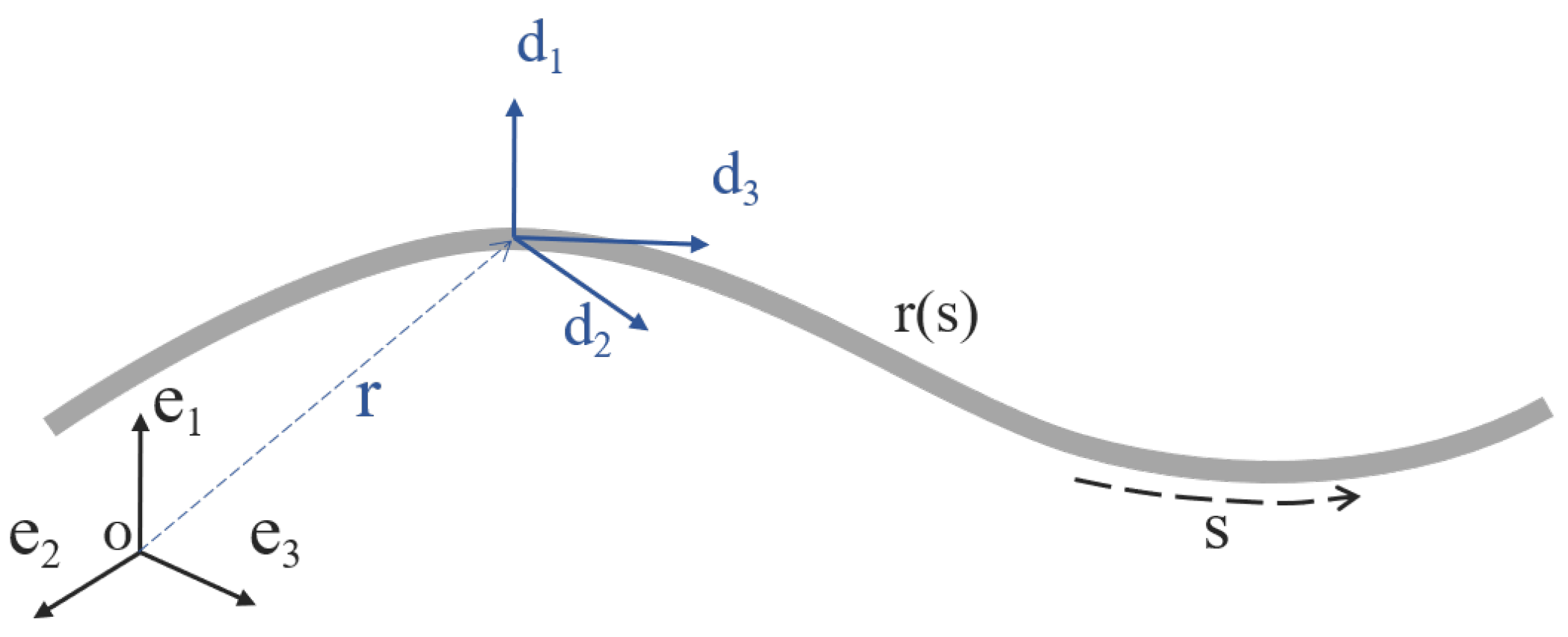
2. Cosserat Theory for Homogeneous Cable Simulation

The Cosserat theory [29] is the most well known theory for the simulation of elastic slender objects. Different from other theories based on one-dimensional curve formulations, the Cosserat theory additionally considers a coordinate frame on the three-dimensional curve in order to describe more accurately the cable’s spatial posture deformation, such as shear or torsion, with a reasonable computational budget. It is based on the assumption of the homogeneous material distribution of the cables under study.

Theory behind Cosserat Model

In the Cosserat theory, the elastic rod is described as a continuous one-dimensional curve $\mathbf{r}\left(s\right)$ in 3D space, for a length parameter $s\in [0,L]$, as shown in Figure 1. Local coordinate frames ${\mathbf{d}}_1\left(s\right),{\mathbf{d}}_2\left(s\right),{\mathbf{d}}_3\left(s\right)$ are constructed on a point of the continuous curve $\mathbf{r}\left(s\right)$, where ${\mathbf{d}}_1$ is along the tangent direction of the curve, ${\mathbf{d}}_2$ is along the principal normal direction of the curve, and ${\mathbf{d}}_3$ is along the binormal direction of the curve, as formulated below:

$$\begin{array}{cc}\hfill {\mathbf{d}}_1& =\frac{\mathrm{d}\mathbf{r}}{\mathrm{d}s}/∥\frac{\mathrm{d}\mathbf{r}}{\mathrm{d}s}∥,\hfill \\ \hfill {\mathbf{d}}_2& =\frac{1}{\vartheta }\frac{\mathrm{d}{\mathbf{d}}_1}{\mathrm{d}s},\hfill \\ \hfill {\mathbf{d}}_3& ={\mathbf{d}}_1\times {\mathbf{d}}_2,\hfill \end{array}$$

(1)

where $\vartheta$ is the curvature of the curve at a specific point.

Accordingly, the centerline and local coordinate system of the Cosserat model are then used to define the stretch, shear, bending, and torsion of the elastic rod, so as to construct the deformation energy equation of the elastic rod.

In the Cosserat model framework, $\mathit{\kappa }$ is defined to describe the linear strains of Cosserat rods, while $\mathit{\sigma }$ is defined to describe the angular strain, expressed in the following form in a local coordinate system:

$$\mathit{\kappa }\left(s\right)={\kappa }_1{\mathit{d}}_1+{\kappa }_2{\mathit{d}}_2+{\kappa }_3{\mathit{d}}_3,\mathit{\sigma }\left(s\right)={\sigma }_1{\mathit{d}}_1+{\sigma }_2{\mathit{d}}_2+{\sigma }_3{\mathit{d}}_3,$$

(2)

where ${\kappa }_i$ represents the rotation of the frame around ${\mathit{d}}_i$ for $i=1,2,3$. In particular, ${\kappa }_1$ and ${\kappa }_2$ measure the bending of the rod, and ${\kappa }_3$ measures its torsion. ${\sigma }_1$ and ${\sigma }_2$ represent the shear along ${\mathit{d}}_1$ and ${\mathit{d}}_2$, and ${\sigma }_3$ measures the stretch along ${\mathit{d}}_3$.

The strains $\mathit{\kappa }$ and $\mathit{\sigma }$ can be calculated by the following expression:

$$\mathit{\kappa }\left(s\right)=\mathrm{vec}\left[{(\partial \mathbf{Q}/\partial s)}^{\mathrm{T}}\mathbf{Q}\right],\mathit{\sigma }\left(s\right)=\mathbf{Q}\left(\frac{\partial \mathbf{r}}{\partial s}-{\mathbf{d}}_3\right),$$

(3)

where $\mathrm{vec}\left[\mathbf{A}\right]$ denotes the 3-vector associated with the skew-symmetric matrix, $\mathbf{A}$, $\mathbf{Q}=\{{\mathbf{d}}_1,{\mathbf{d}}_2,{\mathbf{d}}_3\}$. Equation (3) is defined in a local coordinate frame built on the elastic rod.

Assuming that the material is completely elastic, the stress–strain relationship is linear, as can be derived from the linear material constitutive law. According to Kirchhoff’s constitutive law [30,31,32], we define the bending stiffness ($\mathbf{B}$) and shear stiffness ($\mathbf{S}$); the stiffness matrix is a diagonal 3 × 3 matrix,

$$\begin{array}{ccc}\hfill \mathbf{B}\left(s\right)& =\mathrm{diag}\{Y{I}_1,Y{I}_2,G{I}_3\},\mathbf{S}\left(s\right)\hfill & \hfill =\mathrm{diag}\{{\alpha }_{c}GA,{\alpha }_{c}GA,YA\},\end{array}$$

(4)

where Y is the elastic Young’s modulus, G is the shear modulus, A is the area of the section, $I_i$ is the moment of inertia of the section, and the value of the constant ${\alpha }_c$ is related to the shape of the section. Thus, the torque and stress can be expressed as

$$\mathit{\tau }\left(s\right)=\mathbf{B}\left(s\right)(\mathit{\kappa }\left(s\right)-\mathit{\kappa }{\left(s\right)}^{\mathbf{o}}),\mathbf{n}\left(s\right)=\mathbf{S}\left(s\right)(\mathit{\sigma }\left(s\right)-\mathit{\sigma }{\left(s\right)}^{\mathbf{o}}),$$

(5)

where $\mathit{\kappa }{\left(s\right)}^{\mathbf{o}}$ and $\mathit{\sigma }{\left(s\right)}^{\mathbf{o}}$ correspond to the initial posture of the elastic rod.

According to the defined stress and strain, the potential energy equation at any point on the cross-section of the Cosserat rod can be obtained as

$$\mathsf{\Pi }\left(s\right)=\frac{1}{2}[{(\mathit{\kappa }\left(s\right)-\mathit{\kappa }{\left(s\right)}^{\mathbf{o}})}^{\top }\mathit{\tau }\left(s\right)+{(\mathit{\sigma }\left(s\right)-\mathit{\sigma }{\left(s\right)}^{\mathbf{o}})}^{\top }\mathbf{n}\left(s\right)],$$

(6)

and the total potential energy of the rod is given as

$$\mathsf{\Pi }={\int }_0^L\mathsf{\Pi }\left(s\right)ds.$$

(7)

For the discrete Cosserat rod, the potential energy equation on section i is written as

$${\mathsf{\Pi }}_{\mathit{i}}=\frac{1}{2}[{({\mathit{\kappa }}_{\mathit{i}}-{\mathit{\kappa }}_{\mathit{i}}^{\mathbf{o}})}^{\top }{\mathit{\tau }}_{\mathit{i}}+{({\mathit{\sigma }}_{\mathit{i}}-{\mathit{\sigma }}_{\mathit{i}}^{\mathbf{o}})}^{\top }{\mathbf{n}}_{\mathbf{i}}].$$

(8)

Therefore, the total energy of the whole rod can be expressed as

$$\mathsf{\Pi }=\sum _{i=1}^{N-1}\frac{l_i}{2}({\mathsf{\Pi }}_{\mathit{i}}+{\mathsf{\Pi }}_{\mathit{i}+\mathbf{1}}),$$

(9)

where $l_i$ denotes the length of the discrete rod in segment i. The values of $\mathit{\kappa }$ and $\mathit{\sigma }$ in the equilibrium state can be determined by solving the minimum potential energy of the system, thereby enabling the calculation of the centerline $\mathbf{r}\left(s\right)$ of the Cosserat rod.

In order to solve Equation (9), according to the minimum potential energy principle, the external constraints on the bar need to be determined. The constraint conditions mainly include the initial position ${\mathit{r}}_i$ of the rod and the variables ${\mathit{\kappa }}_{\mathit{i}}$ and ${\mathit{\sigma }}_{\mathit{i}}$ obtained from the initial centerline. We then have

$$[\mathit{\kappa },\mathit{\sigma }]=argmin\sum _{i=1}^{N-1}\frac{l_i}{2}({\mathsf{\Pi }}_{\mathit{i}}+{\mathsf{\Pi }}_{\mathit{i}+\mathbf{1}}).$$

(10)

The quasi-Newton algorithm [33] is usually taken to compute the solution of the above optimization problem.

By fully reflecting the cross-section properties of the Cosserat rod, the method of reconstructing the balance Equation (16) of the Cosserat rod not only ensures the simulation speed of the Cosserat model but also greatly optimizes it. The general idea of the hybrid model is elaborated in Section 3.

3. Coarsened-Shell-Based Cosserat Model (CSC)

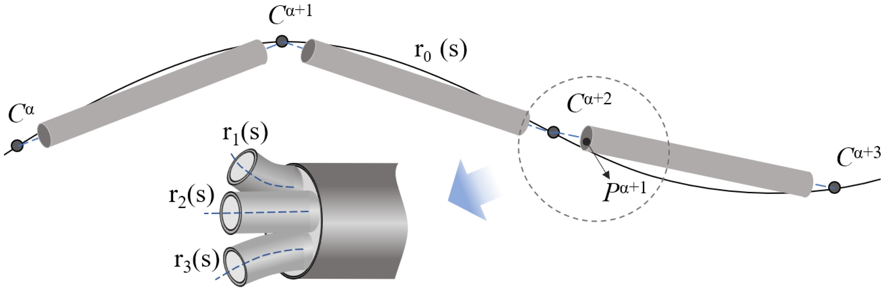
In this section, we build a coarsened-shell-based Cosserat model (CSC) to efficiently capture the behaviors of heterogeneous hybrid cables.

The overall idea is as follows: we first discretize the cables into finite sections as the Cosserat model; then, we compute the potential energy of each section using shell theory; and we finally coarsen the shell simulation by constructing tailored shape functions for an efficiency improvement. The preliminaries, shell simulation procedure, and construction of the coarsened-shell shape functions are elaborated in the following.

3.1. Preliminaries

Consider a cable with centerline curve ${\mathbf{r}}_0\left(s\right)$, where $s\in [0,L]$ is used to parameterize it. It contains $N_r$ interior bundle rods with centerline curves ${\mathbf{r}}_k\left(s\right)(k=1,2,\dots ,N_r)$. The rod is discretized into $N-1$ segments with N heterogeneous section planes $P^{\alpha }(\alpha =1,2,\dots ,N)$ at parameters $s^{\alpha }=\frac{\alpha }{L}$. See also Figure 2.

Each section plane $P^{\alpha }$ is further discretized as a regular fine quadrilateral mesh $\mathcal{M}=\{{\mathcal{M}}^e,e=1,2,\dots ,m\}$ consisting of m fine quadrilateral elements, as plotted in Figure 3a. For later usage in constructing coarsened-shell shape functions, we classify the fine nodes ${\mathcal{X}}_f$ in fine mesh $\mathcal{M}$ into boundary fine nodes and interior fine nodes, denoted by ${\mathcal{X}}_b$ and ${\mathcal{X}}_i$, respectively.

3.2. Shell Simulation Procedure

Taking each heterogeneous section plane $P^{\alpha }$ as a thin shell, its potential energy can be computed by the shell theory, specifically by the Kirchhoff–Love [28] shell formulation, as in this study.

Shape functions act as the basic functions in shell simulation, whose linear combinations are used to describe the deformation of a section plane. Due to the presence of curvature variations in the variational formulation, $C^1$ continuous shape functions are required in the Kirchhoff–Love shell formulation. Thus, the quadratic B-spline basis functions [34] are adopted in the fine mesh $\mathcal{M}$. More precisely, considering a fine node $i\in {\mathcal{X}}_f$ with coordinate ${\mathbf{x}}_i=(x_i,y_i,z_i)$, the associated quadratic B-spline basis function $N^i\left(\mathbf{x}\right)$ is defined as

$$N^i\left(\mathbf{x}\right)=\varphi \left(\frac{x-x_i}{h}\right)\varphi \left(\frac{y-y_i}{h}\right)\varphi \left(\frac{z-z_i}{h}\right),$$

(11)

where h denotes the fine element span and $\varphi (·)$ is the univariate quadratic B-spline basis function [35,36],

$$\varphi \left(\xi \right)=\left\{\begin{array}{cc}\frac{1}{2}{\xi }^2+\frac{3}{2}\xi +\frac{9}{8},\hfill & -\frac{3}{2}\le \xi \le -\frac{1}{2},\hfill \\ -{\xi }^2+\frac{3}{4},\hfill & -\frac{1}{2}\le \xi \le \frac{1}{2},\hfill \\ \frac{1}{2}{\xi }^2-\frac{3}{2}\xi +\frac{9}{8},\hfill & \frac{1}{2}\le \xi \le \frac{3}{2}.\hfill \end{array}\right.$$

(12)

Given any point $\mathbf{x}\in {\mathcal{M}}^e$, its $x-$, $y-$ and $z-$ displacement components $u\left(\mathbf{x}\right)$, $v\left(\mathbf{x}\right)$, and $w\left(\mathbf{x}\right)$ are interpolated using the quadratic B-spline basis functions as

$$\begin{array}{cc}\hfill u\left(\mathbf{x}\right)& =N^1\left(\mathbf{x}\right)u_1+N^2\left(\mathbf{x}\right)u_2+\dots +N^{16}\left(\mathbf{x}\right)u_{16},\hfill \\ \hfill v\left(\mathbf{x}\right)& =N^1\left(\mathbf{x}\right)v_1+N^2\left(\mathbf{x}\right)v_2+\dots +N^{16}\left(\mathbf{x}\right)v_{16},\hfill \\ \hfill w\left(\mathbf{x}\right)& =N^1\left(\mathbf{x}\right)w_1+N^2\left(\mathbf{x}\right)w_2+\dots +N^{16}\left(\mathbf{x}\right)w_{16},\hfill \end{array}$$

(13)

where $(u_i,v_i,w_i)(i=1,2,\dots ,16)$ denotes the displacements of 16 nodes associated with ${\mathcal{M}}^e$. By rewriting the above equation in matrix form, we have the displacement $\mathbf{u}\left(\mathbf{x}\right)={(u\left(\mathbf{x}\right),v\left(\mathbf{x}\right),w\left(\mathbf{x}\right))}^T$ at point $\mathbf{x}$ as

$$\begin{array}{cc}\hfill \mathbf{u}\left(\mathbf{x}\right)& =\left[\begin{array}{ccccccc}{N}^1\left(\mathbf{x}\right)& 0& 0& \dots & N^{16}\left(\mathbf{x}\right)& 0& 0\\ 0& N^1\left(\mathbf{x}\right)& 0& \dots & 0& N^{16}\left(\mathbf{x}\right)& 0\\ 0& 0& N^1\left(\mathbf{x}\right)& \dots & 0& 0& N^{16}\left(\mathbf{x}\right)\end{array}\right]{\mathbf{q}}^e\hfill \\ \hfill & ={\mathbf{N}}^e\left(\mathbf{x}\right){\mathbf{q}}^e,\hfill \end{array}$$

(14)

where ${\mathbf{N}}^e\left(\mathbf{x}\right)$ of size $(3\times 48)$ denotes the element shape function matrix and ${\mathbf{q}}^e$ of size $(48\times 1)$ is the displacement vector of element ${\mathcal{M}}^e$. Assembling ${\mathbf{N}}^e\left(\mathbf{x}\right)$ for all fine elements ${\mathcal{M}}^e,1\le e\le m$, we obtain the shape function matrix ${\mathbf{N}}^h\left(\mathbf{x}\right)$ in fine mesh $\mathcal{M}$,

$${\mathbf{N}}^h\left(\mathbf{x}\right)=\sum _{e=1}^m{\mathbf{N}}^e\left(\mathbf{x}\right),\mathbf{x}\in P^{\alpha }.$$

(15)

Using the above shape function matrix ${\mathbf{N}}^h\left(\mathbf{x}\right)$, the potential energy at the section $P^{\alpha }$ can be computed based on shell theory [28],

$${\tilde{\mathsf{\Pi }}}^{\alpha }=\frac{1}{2}{\int }_{P^{\alpha }}\mathit{n}:\mathit{\epsilon }+\mathit{m}:\mathit{\kappa }\mathrm{d}\mathsf{\Omega }-{\int }_{P^{\alpha }}\mathbf{f}·\mathbf{u}\mathbf{d}\mathsf{\Omega },$$

(16)

where $\mathbf{u}$ denotes the displacement, $\mathit{n}$ and $\mathit{m}$ are the membrane stresses and bending moments, $\mathit{\epsilon }$ and $\mathit{\kappa }$ are the membrane strain and bending strain, $\mathbf{f}$ is the enforced body force, and the notation $(\stackrel{ }{˜})$ is used to distinguish from the energy obtained by the Cosserat model.

Directly employing the fine mesh mentioned above would yield high-fidelity solutions, but it would also bring high computational costs due to the large number of DOFs. On the other hand, the Cosserat model takes a rod as a homogeneous material, which results in a considerable loss in simulation accuracy. This study addresses this issue by introducing the CSC model, as discussed below.

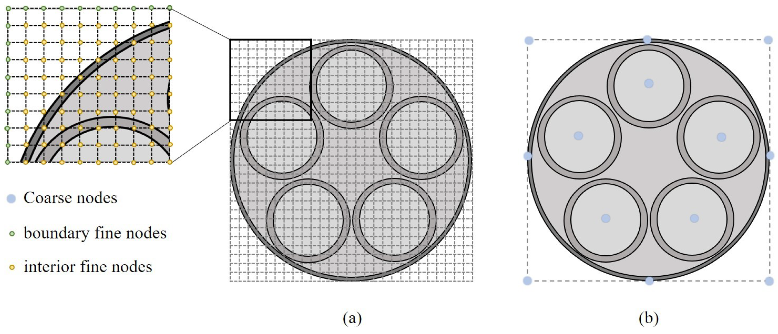
3.3. Coarsened-Shell Shape Functions

In the fine mesh of each section plane $P^{\alpha }$, a set of $r^{\prime }$ equally spaced nodes on its boundary (8 nodes in Figure 3b), coupled with $N_r$ nodes at ${\mathbf{r}}_k\left(s^{\alpha }\right)(k=1,2,\dots ,N_r)$, forms $r=r^{\prime }+N_r$ coarse nodes ${\mathcal{X}}^{\alpha }$.

In the proposed CSC model, the displacements ${\mathbf{Q}}^{\alpha }$ at coarse nodes are taken as DOFs and a set of coarsened-shell shape functions ${\mathbf{N}}^{\alpha }$ is constructed for coarse nodes ${\mathcal{X}}^{\alpha }$, as a combination of the quadratic B-spline shape functions, in each section plane $P^{\alpha }$,

$${\mathbf{N}}^{\alpha }\left(\mathbf{x}\right)={\mathbf{N}}^h\left(\mathbf{x}\right){\mathsf{\Phi }}^{\alpha },$$

(17)

where ${\mathsf{\Phi }}^{\alpha }$ is a matrix to be determined for the purpose of closely capturing the distribution of the hybrid heterogeneous material in the section plane, and the shape function matrix ${\mathbf{N}}^h\left(\mathbf{x}\right)$ in the fine mesh $\mathcal{M}$ refers to Equation (15).

Using the coarsened-shell shape functions ${\mathbf{N}}^{\alpha }\left(\mathbf{x}\right)$, the displacement of any point $\mathbf{x}\in P^{\alpha }$ can be obtained as

$$\mathbf{u}\left(\mathbf{x}\right)={\mathbf{N}}^{\alpha }\left(\mathbf{x}\right){\mathbf{Q}}^{\alpha },\mathbf{x}\in P^{\alpha }.$$

(18)

Further, the potential energy is computed using the proposed shape functions ${\mathbf{N}}^{\alpha }\left(\mathbf{x}\right)$ as in Equation (16).

The critical remaining question is how to determine the matrix ${\mathsf{\Phi }}^{\alpha }$ so as to consider the distribution of the internal material. Instead of formulating it as a constrained nonlinear optimization problem [9], we construct ${\mathsf{\Phi }}^{\alpha }$ as a mapping from the displacements ${\mathbf{Q}}^{\alpha }$ of coarse nodes to the displacements ${\mathbf{q}}^{\alpha }$ of fine nodes in $P^{\alpha }$,

$${\mathbf{q}}^{\alpha }={\mathsf{\Phi }}^{\alpha }{\mathbf{Q}}^{\alpha }.$$

(19)

This is achieved in two steps: first, the displacements ${\mathbf{Q}}^{\alpha }$ of coarse nodes ${\mathcal{X}}^{\alpha }$ are mapped to those ${\mathbf{q}}_b$ of boundary fine nodes ${\mathcal{X}}_b$ using the moving least squares (MLS) interpolation matrix ${\mathsf{\Psi }}^{\alpha }$; then, the displacements ${\mathbf{q}}_b$ of boundary fine nodes ${\mathcal{X}}_b$ are mapped to those ${\mathbf{q}}_i$ of interior fine nodes ${\mathcal{X}}_i$ using the shell transformation matrix ${\mathbf{M}}^{\alpha }$, i.e.,

$${\mathbf{q}}^{\alpha }={\mathbf{M}}^{\alpha }{\mathbf{q}}_b,{\mathbf{q}}_b={\mathsf{\Psi }}^{\alpha }{\mathbf{Q}}^{\alpha }.$$

(20)

Multiplying the matrix ${\mathbf{M}}^{\alpha }$ and ${\mathsf{\Psi }}^{\alpha }$ gives the matrix ${\mathsf{\Phi }}^{\alpha }$ satisfying Equation (19):

$${\mathsf{\Phi }}^{\alpha }={\mathbf{M}}^{\alpha }{\mathsf{\Psi }}^{\alpha }.$$

(21)

The construction details of the MLS interpolation matrix and shell transformation matrix are explained in the next section.

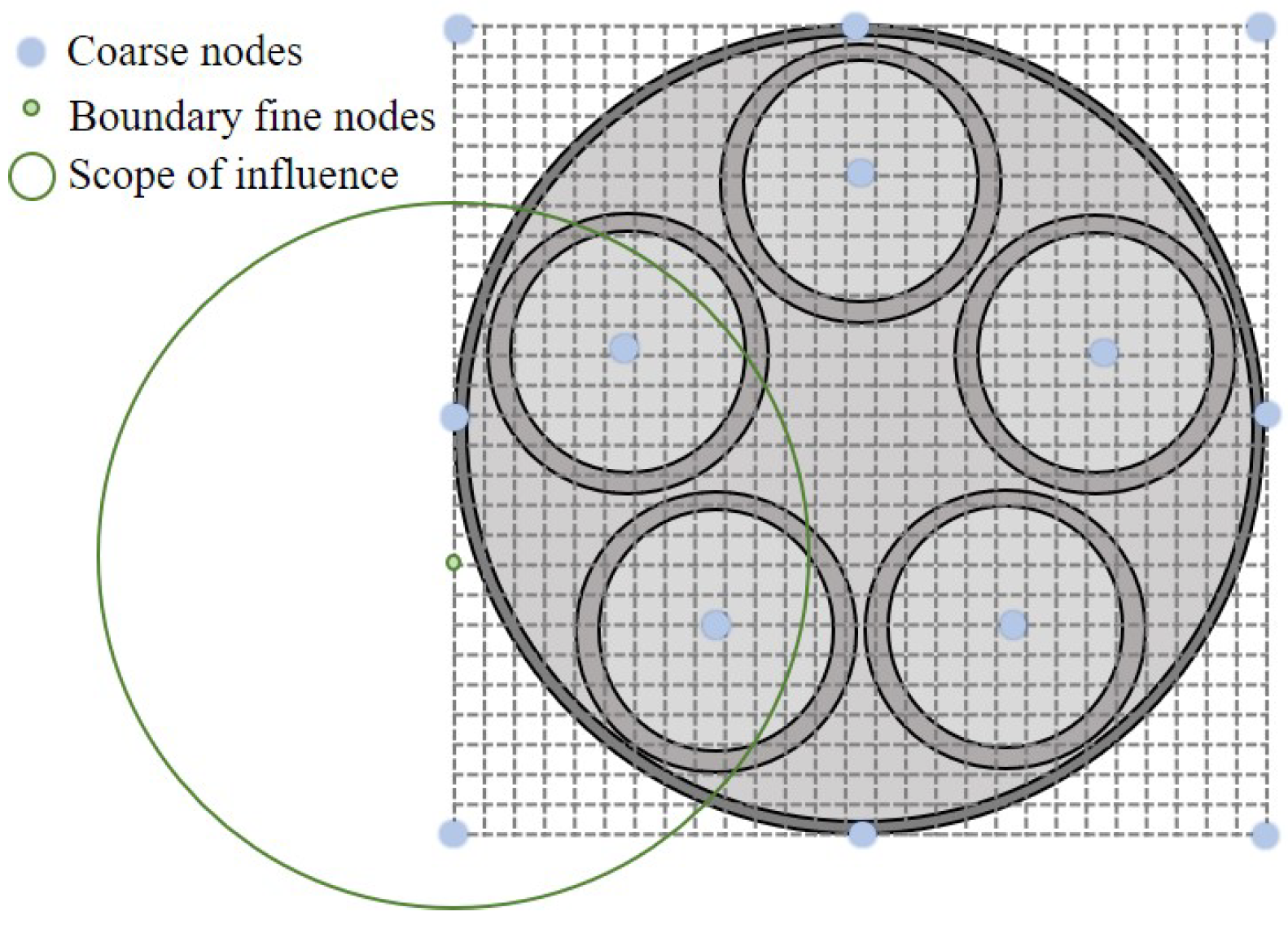
4. Numerical Construction of Coarsened-Shell Shape Functions

The construction procedure of coarsened-shell shape functions ${\mathbf{N}}^{\alpha }\left(\mathbf{x}\right)$ is explained next, consisting of the MLS interpolation matrix in Section 4.1 and the shell transformation matrix in Section 4.2.

4.1. MLS Interpolation Matrix

In this section, the moving least squares (MLS) [37,38] interpolation method is employed to construct a map from the displacements ${\mathbf{Q}}^{\alpha }$ of coarse nodes ${\mathcal{X}}^{\alpha }$ to those ${\mathbf{q}}_b$ of boundary fine nodes ${\mathcal{X}}_b$.

As shown in Figure 4, given any boundary fine node ${\mathbf{x}}_0$, MLS is used to reconstruct a continuous function $h\left({\mathbf{x}}_0\right)$ considering the data $h_I$ located at coarse nodes ${\mathcal{X}}^{\alpha }$,

$$\begin{array}{cc}\hfill h\left({\mathbf{x}}_0\right)& =\sum _j^P{b}_j\left({\mathbf{x}}_0\right)c_j\hfill \\ \hfill & ={\mathbf{b}}^T\left({\mathbf{x}}_0\right)\mathbf{c},\hfill \end{array}$$

(22)

where $\mathbf{b}\left(\mathbf{x}\right)$ and $\mathbf{c}$ denote the basis vector containing monomials up to degree p and the vector of coefficients, respectively,

$$\begin{array}{cc}\hfill \mathbf{b}\left(\mathbf{x}\right)& ={[1,x,y,z,xy,yz,xz,xyz,\dots ]}^T,\hfill \\ \hfill \mathbf{c}& ={[c_1,c_2,\dots ,c_P]}^T,\hfill \end{array}$$

(23)

both having a size of $P={(p+1)}^3$.

To solve for the unknown coefficients of the polynomial fit, the following objective function is constructed:

$$\mathcal{R}=\sum _I^{r}w\left({\mathbf{x}}_I-{\mathbf{x}}_0\right){\left(\sum _j^P{b}_j\left({\mathbf{x}}_I\right)c_j-h_I\right)}^2,$$

(24)

where $w\left(\mathbf{x}\right)$ is the weight function, designed to be the maximum at 0 and drop off to zero at a search radius R,

$$w\left(\mathbf{x}\right)=\left\{\begin{array}{cc}1-\frac{{\left|\right|\mathbf{x}\left|\right|}_2}{R},\hfill & {\left|\right|\mathbf{x}\left|\right|}_2\le R,\hfill \\ 0,\hfill & {\left|\right|\mathbf{x}\left|\right|}_2>R.\hfill \end{array}\right.$$

(25)

By minimizing the above objective function in Equation (24) with regard to the coefficients $\mathbf{c}$, $\frac{\partial \mathcal{R}}{\partial c_k}=0,k=1,2,\dots ,P$ is set to give the normal equations

$$\begin{array}{cc}\hfill & \sum _I^r\left(b_k\left({\mathbf{x}}_I\right)w\left({\mathbf{x}}_I-{\mathbf{x}}_0\right)\sum _j^P{c}_j{b}_j\left({\mathbf{x}}_I\right)\right)\hfill \\ \hfill =& \sum _I^r{b}_k\left({\mathbf{x}}_I\right)w\left({\mathbf{x}}_I-{\mathbf{x}}_0\right)h_I.\hfill \end{array}$$

(26)

By solving the above normal equations, the MLS interpolation functions ${\psi }_I\left({\mathbf{x}}_0\right)$ at ${\mathbf{x}}_0$ are computed as

$${\psi }_I\left({\mathbf{x}}_0\right)={\mathbf{b}}^T\left({\mathbf{x}}_0\right){\mathbf{H}}^{-1}\left({\mathbf{x}}_0\right)\mathbf{b}\left({\mathbf{x}}_I\right)w({\mathbf{x}}_I-{\mathbf{x}}_0),$$

(27)

where the matrix $\mathbf{H}$ is defined as

$$\mathbf{H}\left({\mathbf{x}}_0\right)=\sum _I^{r}w({\mathbf{x}}_I-{\mathbf{x}}_0)\mathbf{b}\left({\mathbf{x}}_I\right)\mathbf{b}{\left({\mathbf{x}}_I\right)}^T.$$

(28)

Using the above MLS interpolation functions ${\psi }_I\left({\mathbf{x}}_0\right)$ in Equation (27), the displacement $\mathbf{u}\left({\mathbf{x}}_0\right)$ at ${\mathbf{x}}_0$ can be interpolated by the displacements ${\mathbf{Q}}^{\alpha }$ at coarse nodes ${\mathcal{X}}^{\alpha }$ as

$$\mathbf{u}\left({\mathbf{x}}_0\right)=\sum _I^r{\psi }_I\left({\mathbf{x}}_0\right){\mathbf{Q}}^I,$$

(29)

or by writing it in the matrix form

$$\begin{array}{cc}\hfill \mathbf{u}\left({\mathbf{x}}_0\right)& =\left[\begin{array}{c}\begin{array}{ccccccc}{\psi }_1\left({\mathbf{x}}_0\right)& 0& 0& \dots & {\psi }_r\left({\mathbf{x}}_0\right)& 0& 0\\ 0& {\psi }_1\left({\mathbf{x}}_0\right)& 0& \dots & 0& {\psi }_r\left({\mathbf{x}}_0\right)& 0\\ 0& 0& {\psi }_1\left({\mathbf{x}}_0\right)& \dots & 0& 0& {\psi }_r\left({\mathbf{x}}_0\right)\end{array}\end{array}\right]{\mathbf{Q}}^{\alpha }\hfill \\ \hfill & =\mathit{\psi }\left({\mathbf{x}}_0\right){\mathbf{Q}}^{\alpha }.\hfill \end{array}$$

(30)

By repeating the above MLS interpolation process for each boundary fine node ${\mathbf{x}}_0\in {\mathcal{X}}_b$, the desired MLS interpolation matrix ${\mathsf{\Psi }}^{\alpha }$ is obtained as

$${\mathsf{\Psi }}^{\alpha }=[\mathit{\psi }\left({\mathbf{x}}_0\right),{\mathbf{x}}_0\in {\mathcal{X}}_b].$$

(31)

4.2. Shell Transformation Matrix

In this section, a shell simulation in the fine mesh $\mathcal{M}$ is solved and then static condensation is applied to map the displacements ${\mathbf{q}}_b$ of boundary fine nodes ${\mathcal{X}}_b$ to those ${\mathbf{q}}_i$ of interior fine nodes ${\mathcal{X}}_i$.

More precisely, each section plane $P^{\alpha }$ is taken as a thin shell and solved using the Kirchhoff–Love shell formulation. In the theory of the Kirchhoff–Love shell, transverse shear strain deformation is neglected and a vector normal to the mid-surface remains normal after deformation. By using the curvilinear coordinate $({\xi }^1,{\xi }^2,{\xi }^3)$, the shell $P^{\alpha }$ is represented as

$$\mathbf{x}({\xi }^1,{\xi }^2,{\xi }^3)=\mathbf{r}({\xi }^1,{\xi }^2)+{\xi }^3{\mathbf{a}}_3({\xi }^1,{\xi }^2),$$

(32)

where $\mathbf{r}({\xi }^1,{\xi }^2)$ denotes the mid-surface of the shell, ${\mathbf{a}}_3$ is the unit normal vector to the mid-surface, and ${\xi }^3$ is the coordinate in the thickness direction ($-0.5t\le {\xi }^3\le 0.5t$ with t set as the shell thickness). The deformed and undeformed configurations are denoted by $\mathbf{x},\mathbf{r}$ and $\mathbf{X},\mathbf{R}$, respectively. The covariant basis vectors of the mid-surface and normal vector are then

$${\mathbf{a}}_{\alpha }=\frac{\partial \mathbf{r}}{\partial {\xi }^{\alpha }},{\mathbf{a}}_3=\frac{{\mathbf{a}}_1\times {\mathbf{a}}_2}{\left|{\mathbf{a}}_1\times {\mathbf{a}}_2\right|},$$

(33)

where $\alpha =1,2$. The covariant metric coefficients $a_{\alpha \beta }$ and the curvature tensor coefficients $b_{\alpha \beta }$ are defined as

$$a_{\alpha \beta }={\mathbf{a}}_{\alpha }·{\mathbf{a}}_{\beta },b_{\alpha \beta }={\mathbf{a}}_3·{\mathbf{a}}_{\alpha ,\beta }.$$

(34)

Based on the above definitions, the Green–Lagrange strain $E_{\alpha ,\beta }$ is obtained by

$$E_{\alpha \beta }={\epsilon }_{\alpha \beta }+{\xi }_3{\kappa }_{\alpha \beta },$$

(35)

where ${\epsilon }_{\alpha \beta },{\kappa }_{\alpha \beta }$ are the membrane strains and bending strains, respectively,

$$\begin{array}{cc}\hfill {\epsilon }_{\alpha \beta }& =\frac{1}{2}\left(a_{\alpha \beta }-A_{\alpha \beta }\right)\hfill \\ \hfill {\kappa }_{\alpha \beta }& =b_{\alpha \beta }-B_{\alpha \beta },\hfill \end{array}$$

(36)

where $a_{\alpha \beta },b_{\alpha \beta }$ and $A_{\alpha \beta },B_{\alpha \beta }$ denote the corresponding coefficients in the deformed and undeformed configurations, i.e., computed on the deformed mid-surface $\mathbf{r}$ and undeformed mid-surface $\mathbf{R}$. For the linear elastic material considered here, the membrane stresses $n_{\alpha \beta }$ and bending moments $m_{\alpha \beta }$ are then given as

$$\begin{array}{cc}\hfill \left[\begin{array}{c}{\overline{n}}_{11}\hfill \\ {\overline{n}}_{22}\hfill \\ {\overline{n}}_{12}\hfill \end{array}\right]& =\frac{Et}{1-v^2}\left[\begin{array}{ccc}1& v& 0\\ v& 1& 0\\ 0& 0& \frac{1-v}{2}\end{array}\right]\left[\begin{array}{c}{\overline{\epsilon }}_{11}\\ {\overline{\epsilon }}_{22}\\ 2{\overline{\epsilon }}_{12}\end{array}\right],\hfill \\ \hfill \left[\begin{array}{c}{\overline{m}}_{11}\hfill \\ {\overline{m}}_{22}\hfill \\ {\overline{m}}_{12}\hfill \end{array}\right]& =\frac{E{t}^3}{12\left(1-v^2\right)}\left[\begin{array}{ccc}1& v& 0\\ v& 1& 0\\ 0& 0& \frac{1-v}{2}\end{array}\right]\left[\begin{array}{c}{\overline{\kappa }}_{11}\\ {\overline{\kappa }}_{22}\\ 2{\overline{\kappa }}_{12}\end{array}\right],\hfill \end{array}$$

(37)

where E is the Young’s modulus, v is the Poisson’s ratio, and the notation $(\stackrel{ }{¯})$ refers to values on a local Cartesian basis.

Using the principle of virtual work [39] to define the variational formulation for the Kirchhoff–Love shell problem, the variations in the internal work $W^{int}$ and external work $W^{ext}$ are defined as

$$\begin{array}{cc}\hfill \delta \tilde{\mathsf{\Pi }}(\mathbf{u},\delta \mathbf{u})& =\delta {\tilde{\mathsf{\Pi }}}^{\mathrm{int}}-\delta {\tilde{\mathsf{\Pi }}}^{\mathrm{ext}}={\int }_{\mathsf{\Omega }}\mathit{n}:\delta \mathit{\epsilon }+\mathit{m}:\delta \mathit{\kappa }\mathrm{d}\mathsf{\Omega }-{\int }_{\mathsf{\Omega }}\mathbf{f}·\delta \mathbf{u}\mathbf{d}\mathsf{\Omega },\hfill \end{array}$$

(38)

where $\mathbf{u}$ denotes the displacement, $\delta \mathbf{u}$ is the virtual displacement, $\delta \mathit{\epsilon }$ is the virtual membrane strain, $\delta \mathit{\kappa }$ is the virtual bending strain, and $\mathbf{f}$ is the enforced body force.

In this fine quadrilateral mesh with n nodes, ${\mathbf{q}}_i,i=1,2,\dots ,n$ are the discretized nodal displacements and $N^i\left(\mathbf{x}\right)$ the corresponding $C^1$-continuous B-spline shape functions in Equation (11). Following the classical Galerkin method [40], the shell displacements are represented by a linear combination of basis functions $N^i\left(\mathbf{x}\right)$,

$$\mathbf{u}\left(\mathbf{x}\right)=\sum _i{N}^i\left(\mathbf{x}\right){\mathbf{q}}_i.$$

(39)

Using the B-spline shape functions $N^i\left(\mathbf{x}\right)$, the first derivatives of the covariant basis vectors $\frac{\partial {\mathbf{a}}_{\alpha }}{\partial u_r}$ in Equation (33) with respect to the displacements $u_r$ are computed as

$$\frac{\partial {\mathbf{a}}_{\alpha }}{\partial u_r}=\frac{\partial \left({\mathbf{R}}_{,\alpha }+{\mathbf{u}}_{,\alpha }\right)}{\partial u_r}=\frac{\partial {\mathbf{u}}_{,\alpha }}{\partial u_r}=\sum _{i=1}^n{N}_{,\alpha }^i\frac{\partial {\mathbf{q}}_i}{\partial u_r}.$$

(40)

Taking the first and second derivatives of the virtual work obtains the residual vector ${\mathbf{R}}^h$ and tangent stiffness matrix ${\mathbf{K}}^h$ (the superscript $\alpha$ is omitted for clarity),

$$\begin{array}{cc}\hfill R_i^h=& {\int }_{\mathsf{\Omega }}\mathit{n}:\frac{\partial \mathit{\epsilon }}{\partial q_i}+\mathit{m}:\frac{\partial \mathit{\kappa }}{\partial q_i}\mathrm{d}\mathsf{\Omega }-{\int }_{\mathsf{\Omega }}\mathbf{f}·\frac{\partial \mathbf{u}}{\partial q_i}\mathrm{d}\mathsf{\Omega },\hfill \\ \hfill K_{ij}^h=& {\int }_{\mathsf{\Omega }}\frac{\partial \mathit{n}}{\partial q_j}:\frac{\partial \mathit{\epsilon }}{\partial q_i}+\mathit{n}:\frac{{\partial }^2\mathit{\epsilon }}{\partial q_i\partial q_j}+\frac{\partial \mathit{m}}{\partial q_j}:\frac{\partial \mathit{\kappa }}{\partial q_i}\hfill \\ \hfill & +\mathit{m}:\frac{{\partial }^2\mathit{\kappa }}{\partial q_i\partial q_j}\mathrm{d}\mathsf{\Omega }.\hfill \end{array}$$

(41)

Then, the displacements ${\mathbf{q}}^{\alpha }$ can be solved by solving the following linear system:

$${\mathbf{K}}^h{\mathbf{q}}^{\alpha }=-{\mathbf{R}}^h.$$

(42)

By classifying the displacements ${\mathbf{q}}^{\alpha }$ of fine nodes into ${\mathbf{q}}_b$ of boundary fine nodes ${\mathcal{X}}_b$ and ${\mathbf{q}}_i$ of interior fine nodes ${\mathcal{X}}_i$, the above equation can be rearranged as

$$\left[\begin{array}{cc}{\mathbf{k}}_b& {\mathbf{k}}_{bi}\\ {\mathbf{k}}_{ib}& {\mathbf{k}}_i\end{array}\right]\left[\begin{array}{c}{\mathbf{q}}_b\hfill \\ {\mathbf{q}}_i\hfill \end{array}\right]=\left[\begin{array}{c}{\mathbf{R}}_b\\ {\mathbf{R}}_i\end{array}\right],$$

(43)

where ${\mathbf{k}}_b,{\mathbf{k}}_{bi},{\mathbf{k}}_{ib},{\mathbf{k}}_i$ and ${\mathbf{R}}_b,{\mathbf{R}}_i$ are the associated sub-matrices/sub-vectors in ${\mathbf{K}}^h$ and ${\mathbf{R}}^h$, respectively. Assuming ${\mathbf{R}}_i=0$, the following equation can be obtained:

$$\begin{array}{cc}\hfill {\mathbf{q}}^{\alpha }& =\left[\begin{array}{c}{\mathbf{q}}_b\\ {\mathbf{q}}_i\end{array}\right]=\left[\begin{array}{c}\mathbf{I}\\ -{\mathbf{k}}_i^{-1}{\mathbf{k}}_{i,b}\end{array}\right]{\mathbf{q}}_b={\mathbf{M}}^{\alpha }{\mathbf{q}}_b,\mathrm{for}{\mathbf{M}}^{\alpha }=\left[\begin{array}{c}\mathbf{I}\\ -{\mathbf{k}}_i^{-1}{\mathbf{k}}_{i,b}\end{array}\right],\hfill \end{array}$$

(44)

where $\mathbf{I}$ is an identity matrix, and ${\mathbf{M}}^{\alpha }$ is the desired shell transformation matrix.

4.3. Usage of Coarsened-Shell Shape Functions in Hybrid Cable Simulation

Based on the above explanations in Section 4.1 and Section 4.2, the proposed coarsened-shell shape functions ${\mathbf{N}}^{\alpha }\left(\mathbf{x}\right)$ are represented as

$${\mathbf{N}}^{\alpha }\left(\mathbf{x}\right)={\mathbf{N}}^h\left(\mathbf{x}\right){\mathsf{\Phi }}^{\alpha }={\mathbf{N}}^h\left(\mathbf{x}\right){\mathbf{M}}^{\alpha }{\mathsf{\Psi }}^{\alpha }.$$

(45)

It is reasonable to conclude that the proposed shape functions are able to approximate the high-fidelity displacements ${\mathbf{q}}^{\alpha }$ of fine nodes using those ${\mathbf{Q}}^{\alpha }$ of the coarse nodes,

$$\begin{array}{cc}\hfill \mathbf{u}\left(\mathbf{x}\right)& ={\mathbf{N}}^{\alpha }\left(\mathbf{x}\right){\mathbf{Q}}^{\alpha }\hfill \\ \hfill & ={\mathbf{N}}^h\left(\mathbf{x}\right){\mathbf{M}}^{\alpha }{\mathsf{\Psi }}^{\alpha }{\mathbf{Q}}^{\alpha }\hfill \\ \hfill & ={\mathbf{N}}^h\left(\mathbf{x}\right){\mathbf{M}}^{\alpha }{\mathbf{q}}_b\hfill \\ \hfill & ={\mathbf{N}}^h\left(\mathbf{x}\right){\mathbf{q}}^{\alpha }.\hfill \end{array}$$

(46)

Thus, the employment of the proposed shape functions ${\mathbf{N}}^{\alpha }$ provides high accuracy at a certain cost of construction.

Now, in each section plane, taking the displacements ${\mathbf{Q}}^{\alpha }$ of coarse nodes ${\mathcal{X}}^{\alpha }$ as DOFs and using the coarsened-shell shape functions ${\mathbf{N}}^{\alpha }$, we can similarly compute the derivatives of the covariant basis vectors as in Equation (40), the residual vector ${\mathbf{R}}^{H,\alpha }$, and the stiffness matrix ${\mathbf{K}}^{H,\alpha }$ as in Equation (41). Further, the potential energy ${\tilde{\mathsf{\Pi }}}^{\alpha }$ in Equation (16) of each section is computed in discrete form,

$${\tilde{\mathsf{\Pi }}}^{\alpha }=\frac{1}{2}{\left({\mathbf{Q}}^{\alpha }\right)}^T{\mathbf{K}}^{H,\alpha }{\mathbf{Q}}^{\alpha }-{\left({\mathbf{Q}}^{\alpha }\right)}^T{\mathbf{R}}^{H,\alpha }.$$

(47)

Based on this, the displacements $\mathbf{Q}$ of coarse nodes from all section planes can be computed by minimizing the total potential $\tilde{\mathsf{\Pi }}$,

$$\mathbf{Q}=\underset{\mathbf{Q}}{argmin}\sum _{\alpha }{\tilde{\mathsf{\Pi }}}^{\alpha }.$$

(48)

4.4. Properties of Coarsened-Shell Shape Functions

The constructed coarsened-shell shape functions have good properties of $C^1$-continuity and the partition of unity, which are important in avoiding un-physical simulation effects [41,42].

In addition, the basic geometric properties of shape functions, such as the partition of unity, are seldom explored in previous studies, and thus they may inevitably produce un-physical results [41]. In order to better exploit the anisotropic behavior of complex heterogeneous objects, matrix-valued shape functions [9] are introduced to account for interactions among quantities along different axes. A similar matrix form is also adopted in this study.

$C^1$-continuity. Benefiting from the B-spline basis functions in the fine mesh, the proposed shape functions are likewise $C^1$ continuous and their first and second derivatives are computed as

$$\begin{array}{cc}\hfill \frac{\partial {\mathbf{N}}^{\alpha }\left(\mathbf{x}\right)}{\partial \mathbf{x}}& =\frac{\partial {\mathbf{N}}^h\left(\mathbf{x}\right)}{\partial \mathbf{x}}{\mathsf{\Phi }}^{\alpha },\hfill \\ \hfill \frac{{\partial }^2{\mathbf{N}}^{\alpha }\left(\mathbf{x}\right)}{\partial {\mathbf{x}}^2}& =\frac{{\partial }^2{\mathbf{N}}^h\left(\mathbf{x}\right)}{\partial {\mathbf{x}}^2}{\mathsf{\Phi }}^{\alpha },\hfill \end{array}$$

(49)

where the above first and second derivatives of the B-spline basis functions are obvious, as in Equations (11) and (12).

Partition of unity. In addition, our proposed shape functions have the partition of unity (PU) property, which avoids non-physical deformations:

$$\begin{array}{cc}\hfill {\mathbf{N}}^{\alpha }\left(\mathbf{x}\right){\mathbf{I}}_{3r}& ={\mathbf{N}}^h\left(\mathbf{x}\right){\mathbf{M}}^{\alpha }{\mathsf{\Psi }}^{\alpha }{\mathbf{I}}_{3r}\hfill \\ \hfill & ={\mathbf{N}}^h\left(\mathbf{x}\right){\mathbf{M}}^{\alpha }{\mathbf{I}}_{3b}\hfill \\ \hfill & ={\mathbf{N}}^h\left(\mathbf{x}\right){\mathbf{I}}_{3b+3i}\hfill \\ \hfill & ={\mathbf{I}}_3,\hfill \end{array}$$

(50)

where ${\mathbf{I}}_n$ denotes a 1-vector of size n, and the following formula representing the PU of MLS interpolation is used:

$${\mathbf{I}}_{3b}={\mathsf{\Psi }}^{\alpha }{\mathbf{I}}_{3r}.$$

(51)

5. Numerical Examples

The performance of the CSC model was also tested using numerical examples. The hybrid cables using FEM, the Cosserat theory, and the proposed CSC model, and their performance, were compared. The FEM results were obtained using the ABAQUS software, version 2021 and used as a benchmark to measure the accuracy. All examples were implemented on an Intel Core i7 PC with a 2.8 GHz CPU and 16 GB RAM (Intel, Santa Clara, CA, USA).

The performance of the tested approach was measured using the following error index $r_u$ to determine their relative solution differences:

$$r_u=\frac{\mid {\mathbf{u}}_1-{\mathbf{u}}_0\mid }{\mid {\mathbf{u}}_0\mid },$$

(52)

where ${\mathbf{u}}_1$ is the calculated displacement and ${\mathbf{u}}_0$ is the reference displacement, while $|·|$ denotes the Euclidean distance.

The approach’s performance was first tested using a typical hybrid cable, shown in Figure 5a, which comprised four small cables of different diameters and of a different material, as shown in

Table 1. The material of each part of the cable model. The unit of the Young’s modulus is MPa.

Index	Material	Young’s Modulus	Poisson’s Ratio
Mat1	rubber	789	0.47
Mat2	nylon	1.4 × 103	0.37
Mat3	copper alloy	1.06 × 105	0.39
Mat4	aluminium alloy	7.1 × 104	0.33

. The initial length of this cable model was 150 mm, and the outer diameter of the bundle was about 30 mm. The cable was fixed on one end, and the other end was subjected to a vertical downward force.

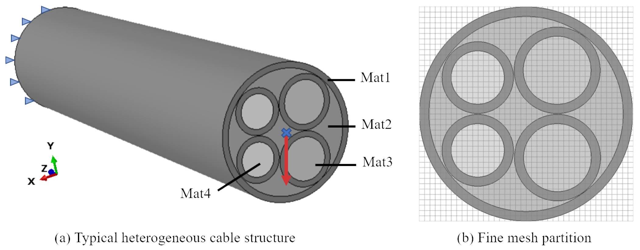
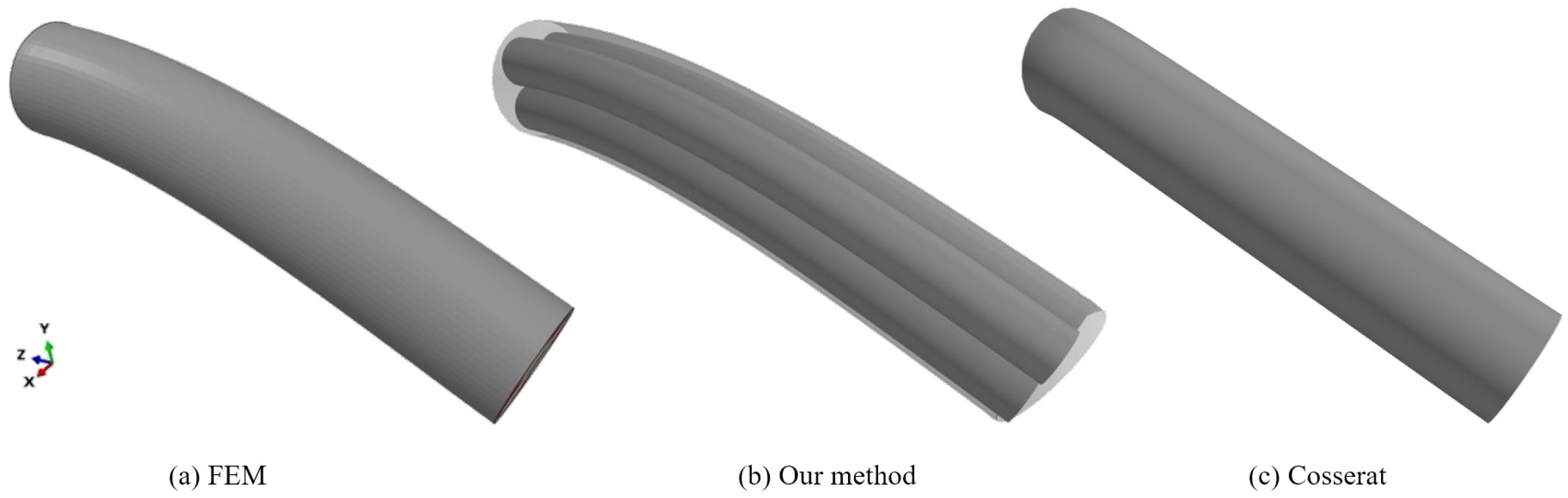
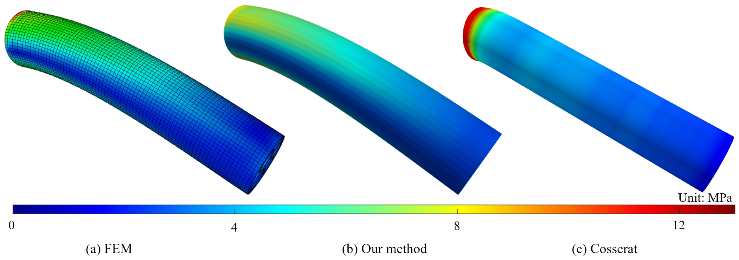
5.1. Comparative Analysis of Same Types of Cables

We first tested the approach’s performance using four small cables of the same material, Mat3; see also Figure 5a. Note that the overall cable was still of a heterogeneous material distribution, including empty areas.

As shown in Figure 5b, in conducting the shell analysis to build the material-aware shape functions, the size of the fine mesh was set to $40\times 40$. The FEM was conducted on the mesh so as to give the benchmark simulation results. Three different simulation results, obtained, respectively, via FEM, the Cosserat theory, and our CSC model, are shown in Figure 6. Their performance is summarized in

Table 2. Simulation accuracy and elapsed time.

Simulation Method	Displacement Error	Elapsed Time (s)
FEM	-	15.2
Our method	0.16	9.7
Cosserat	1.01	4.3

. As can be seen from the results, the Cosserat theory produced quite different results from those of FEM, with an error index of 1.01, while our method was close to FEM, with an error index of 0.16. The latter had a six-times improvement in comparison with the former. The simulation accuracy improvement can also be seen from the deformation comparison in Figure 6, Figure 7 and Figure 8, where we show the deformations and stress distributions for the three different approaches. Cosserat failed to take into account the material anisotropy of the hybrid cables and had a large difference from the benchmark FE results. We also list the computational efficiency in Table 2. Cosserat took 4.3 s, while our CSC method took 9.7 s, as the latter had more DOFs in computing the global displacement. Although our CSC method is slightly slower in computational speed compared to the Cosserat model, the improvement in the simulation accuracy, especially in the accuracy of the stress distribution simulation, is significant. Furthermore, compared to traditional finite element methods, this study increased the solving speed by approximately 36% without compromising the simulation accuracy.

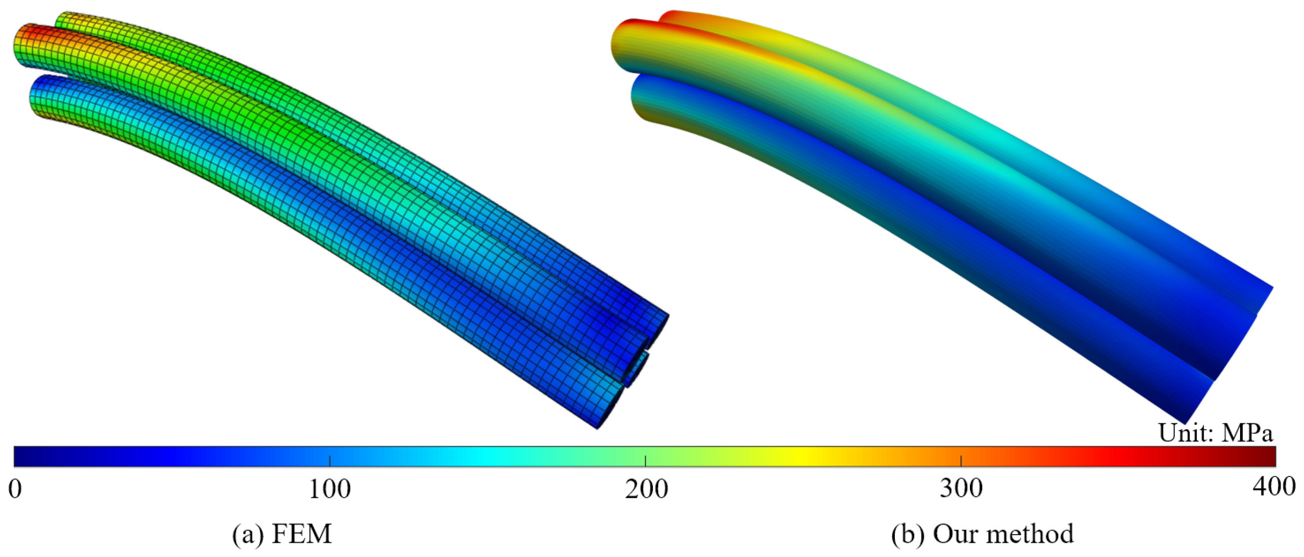
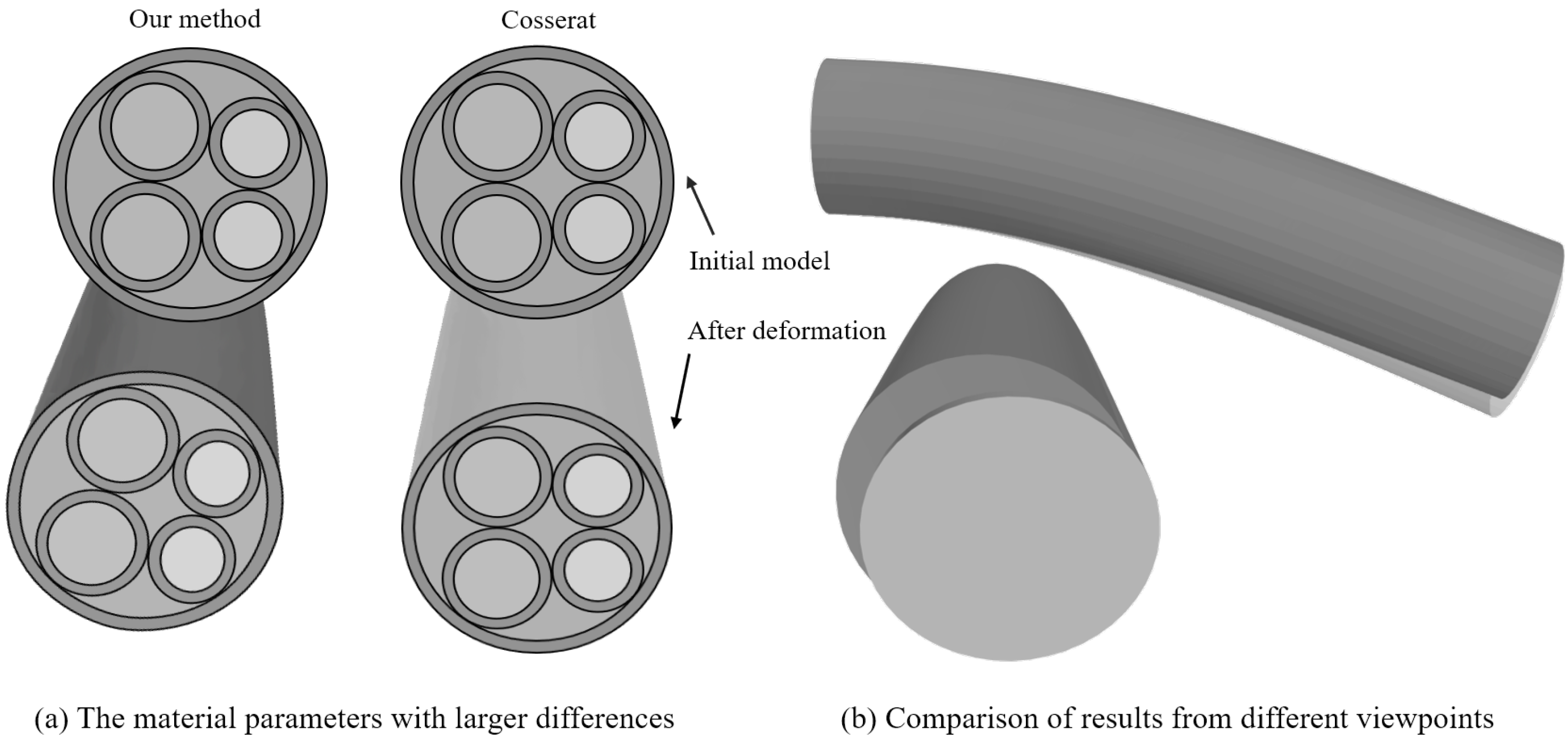
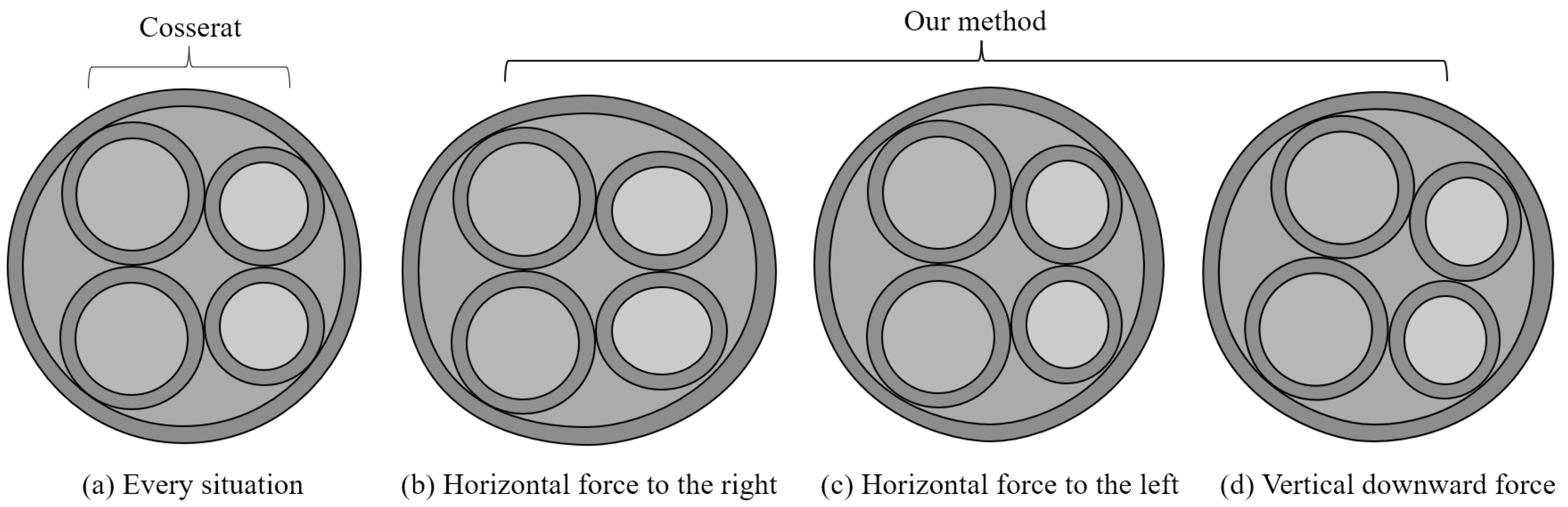
5.2. Comparative Analysis of Different Types of Cables

We also tested the performance of our CSC model for hybrid cables consisting of different types of cables. The object is shown in Figure 5a, with the cable material parameters given in Table 1. Due to the different materials of each wire, the overall cable showed large material anisotropy in the cross-section. The comparisons with the Cosserat results are shown Figure 9 and Figure 10.

As we can see from Figure 9, due to the different material distributions, the cable was tilted toward the “softer” side of the material, although the cable was subjected to a vertical downward force. However, the Cosserat model showed a vertical downward force due to its homogenization in material treatment, resulting in a large error. The Cosserat method had an error index of 3.01 and took 4.1 s, while our CSC method had an error index of 0.17 and took 8.9 s.

The deformations of the hybrid cable are also shown and compared in Figure 10 under different load directions, where (a) gives the section diagram of Cosserat while (b), (c), and (d) give those of our CSC model. Note here that the Cosserat method produced the same cross-section deformation, irrespective of the direction, while ours produced three different ones. The cross-section of the cable was distorted to different degrees due to the heterogeneity of the cable, which was reflected with high accuracy in our approach.

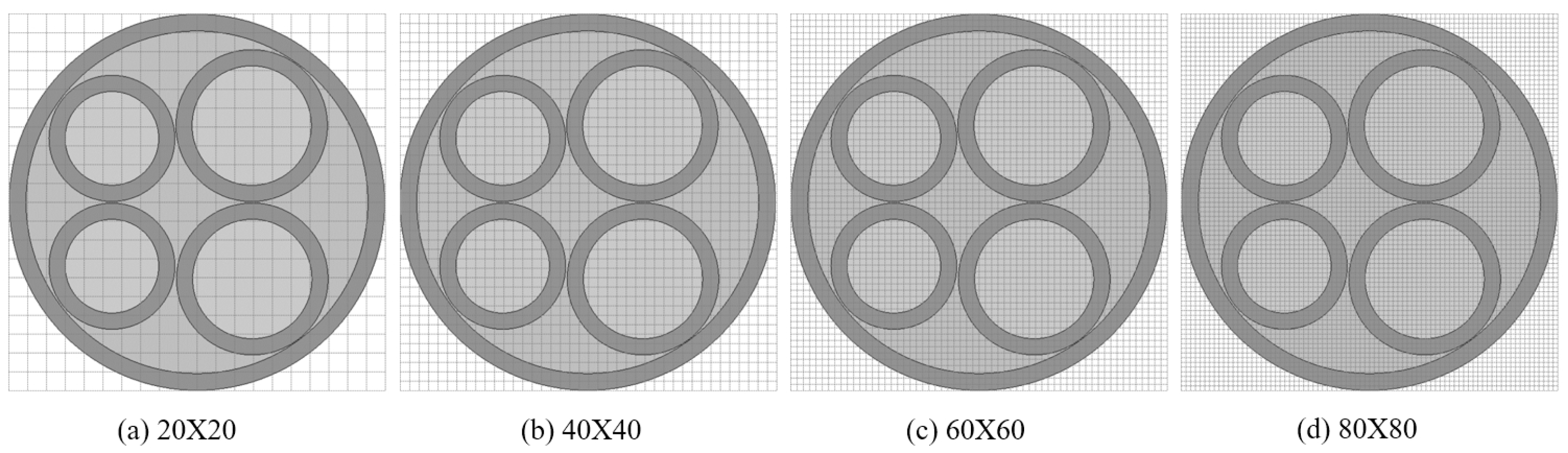
5.3. Performance at Different Mesh Settings

We also tested the CSC model’s performance at different simulation mesh settings, i.e., with variations in the fine mesh size or the number of coarse nodes. The model shown in Figure 5a was again utilized for the test, and the results are shown in Figure 11 and Figure 12.

Different numbers of coarse nodes. The coarse nodes are the primary nodes on the cable section, and the number of coarse nodes can be freely selected to meet different simulation accuracy requirements. We chose coarse node numbers 4, 8, 12, and 16 for the test, and the associated efficiency indices $r_u$ are shown in Figure 11a. The value of the error index decreased rapidly as the number of coarse nodes increased, with reliable convergence.

Fine meshes of different sizes. The fine mesh is set to construct the shape function, as explained in Section 4.2. Four differently sized fine grids of $20\times 20$, $40\times 40$, $60\times 60$, and $80\times 80$ were set; we kept the coarse node number as 8. The result is shown in Figure 12. As can be seen in Figure 11b, the displacement error indices of the proposed CSC method decreased as the number of fine nodes increased, with reliable convergence.

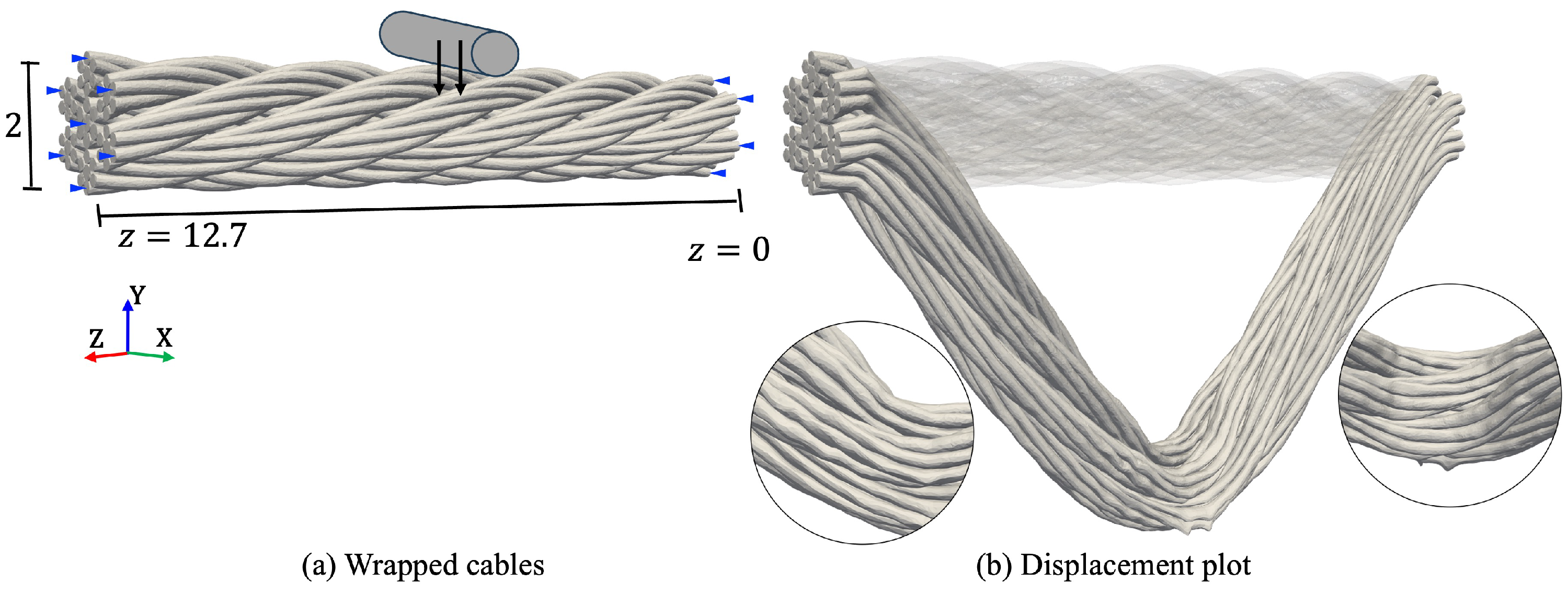
5.4. Complex Wrapped Cables

The ability of the CSC model to capture the deformations of cables exhibiting fine-scale geometric details was tested for the more complex dynamic simulation of a complex wrapped cable, as shown in Figure 13a. The cable consisted of $7\times 7$ bundles and they were composed of aluminium alloy, as shown in Table 1. The cable had a length of 12.7 and a diameter of 2. It was fixed at its two side faces and subjected to a loading field in the vicinity of coordinates ${\mathbf{x}}_0=(0,2,6.35)$, mimicking the contact forces with a cylinder, which can be described as

$$p\left(\mathbf{x}\right)=p_0·\max (0,(1-\left|\right|\mathbf{x}-{\mathbf{x}}_0{\left|\right|}_2\left)\right),\mathrm{for}{p}_0=1\times {10}^6.$$

(53)

Figure 13b shows its reliable displacement result with local details, capturing the behaviors of the different bundles of cables. The simulation used 31.5 K coarse nodes and took 80.7 s in total. Note that this complex cable required a very fine FE mesh consisting of about 100 million DOFs to resolve the geometric details, which precludes its direct usage. The proposed CSC model demonstrated its efficiency in handling such complex details.

6. Conclusions and Prospects

The paper studies the elastic simulation of hybrid cables with heterogeneous material distributions. This research introduces a novel coarsened-shell-based Cosserat (CSC) model that leverages the advantages of the Cosserat model for slender cable representation, incorporates the Kirchhoff–Love shell theory to model cross-sectional deformations, and employs a numerical coarsening approach to reduce the degrees of freedom (DOFs). This approach achieves a high level of simulation accuracy while maintaining the computational efficiency. The CSC model effectively accounts for material anisotropy, as demonstrated through numerical examples comparing it with the classical Cosserat model and benchmark FEM results. This innovative model exhibits significant potential for applications requiring highly accurate simulations of hybrid slender cables with heterogeneous materials. It is important to note that the current implementation of the CSC model is limited to linear elasticity due to the numerical coarsening approach used in modeling cross-sectional deformations. Its extension to the nonlinear elasticity problem still requires efforts to develop novel shape functions to reflect the nonlinear deformation behaviors of the cable’s heterogeneous cross-sections. In the future, we also intend to explore the convergence of the CSC model with advanced shell theories for cross-sectional modeling for more accurate simulation.

References

1. Pai, D. STRANDS: Interactive Simulation of Thin Solids using Cosserat Models. Comput. Graph. Forum 2010, 21, 347–352. [Google Scholar] [CrossRef]
2. Spillmann, J.; Teschner, M. CoRdE: Cosserat rod elements for the dynamic simulation of one-dimensional elastic objects. In Proceedings of the Symposium on Computer Animation, San Diego, CA, USA, 2–4 August 2007. [Google Scholar]
3. Spillmann, J.; Teschner, M. Cosserat Nets. IEEE Trans. Vis. Comput. Graph. 2009, 15, 325–338. [Google Scholar] [CrossRef] [PubMed]
4. Wojtan, C.; Zhao, C.; Lin, J.; Wang, T.; Bao, H.; Huang, J. Efficient and Stable Simulation of Inextensible Cosserat Rods by a Compact Representation. Comput. Graph. Forum 2022, 41, 567–578. [Google Scholar]
5. Bergou, M.; Wardetzky, M.; Robinson, S.; Audoly, B.; Grinspun, E. Discrete elastic rods. In ACM SIGGRAPH 2008 Papers; ACM: New York, NY, USA, 2008; Volume 63, pp. 1–12. [Google Scholar]
6. Weidner, N.; Kyle, P.; Levin, D.; Shinjiro, S. Eulerian-on-lagrangian cloth simulation. ACM Trans. Graph. 2018, 37, 1–11. [Google Scholar] [CrossRef]
7. Linn, J.; Dreler, K. Discrete Cosserat Rod Models Based on the Difference Geometry of Framed Curves for Interactive Simulation of Flexible Cables. In Math for the Digital Factory; Springer: Cham, Switzerland, 2017. [Google Scholar]
8. Smit, R.; Brekelmans, W.; Meijer, H. Prediction of the mechanical behavior of nonlinear heterogeneous systems by multi-level finite element modeling. Comput. Methods Appl. Mech. Eng. 1998, 155, 181–192. [Google Scholar] [CrossRef]
9. Chen, J.; Bao, H.; Wang, T.; Desbrun, M.; Huang, J. Numerical coarsening using discontinuous shape functions. ACM Trans. Graph. 2018, 37, 1–12. [Google Scholar] [CrossRef]
10. Grégoire, M.; Schömer, E. Interactive simulation of one-dimensional flexible parts. Comput.-Aided Des. 2007, 39, 694–707. [Google Scholar] [CrossRef]
11. Baraff, D. Large Steps in Cloth Simulation. In Proceedings of the 25th Annual Conference on Computer Graphics and Interactive Techniques, Orlando, FL, USA, 19–24 July 1998. [Google Scholar]
12. Lv, N.; Liu, J.; Xia, H.; Ma, J.; Yang, X. A review of techniques for modeling flexible cables. Comput.-Aided Des. 2020, 122, 102826. [Google Scholar] [CrossRef]
13. Hermansson, T.; Bohlin, R.; Carlson, J.; Söderberg, R. Automatic assembly path planning for wiring harness installations. J. Manuf. Syst. 2013, 32, 417–422. [Google Scholar] [CrossRef]
14. Stumpp, T.; Spillmann, J.; Becker, M.; Teschner, M. A Geometric Deformation Model for Stable Cloth Simulation. In Proceedings of the Workshop on Virtual Reality Interactions & Physical Simulations, Grenoble, France, 11–12 November 2008. [Google Scholar]
15. Celniker, G.; Gossard, D. Deformable curve and surface finite-elements for free-form shape design. ACM Siggraph Comput. Graph. 1991, 25, 257–266. [Google Scholar] [CrossRef]
16. Hergenrther, E.; Dhne, P.; Rundeturmstr, R. Real-Time Virtual Cables Based on Kinematic Simulation. In Proceedings of the International Conference in Central Europe on Computer Graphics and Visualization, Plzen, Czech Republic, 7–10 February 2000. [Google Scholar]
17. Lv, N.; Liu, J.; Ding, X.; Lin, H. Assembly simulation of multi-branch cables. J. Manuf. Syst. 2017, 45, 201–211. [Google Scholar] [CrossRef]
18. Nordenholz, T.; O’Reilly, O. On steady motions of isotropic, elastic Cosserat points. IMA J. Appl. Math. 1998, 60, 55–72. [Google Scholar] [CrossRef]
19. Wen, J.; Chen, J.; Umetani, N.; Bao, H.; Huang, J. Cosserat Rod with rh-Adaptive Discretization. Comput. Graph. Forum 2020, 39, 143–154. [Google Scholar] [CrossRef]
20. Du, H.; Jiang, Q.; Xiong, W. Computer-assisted assembly process planning for the installation of flexible cables modeled according to a viscoelastic Cosserat rod model. Proc. Inst. Mech. Eng. Part B J. Eng. Manuf. 2023, 237, 1737–1747. [Google Scholar] [CrossRef]
21. Landau, L.; Lifshitz, E. Electrodynamics of Continuous Media; Butterworth Heinemann: Oxford, UK, 1984. [Google Scholar]
22. Li, H.; Leow, W.; Chiu, I. Elastic Tubes: Modeling Elastic Deformation of Hollow Tubes. Comput. Graph. Forum 2010, 29, 1770–1782. [Google Scholar] [CrossRef]
23. Arne, W.; Marheineke, N.; Meister, A.; Wegener, R. Numerical analysis of Cosserat rod and string models for viscous jets in rotational spinning processes. Math. Model. Methods Appl. Sci. 2011, 20, 1941–1965. [Google Scholar] [CrossRef]
24. Li, M.; Hu, J. Analysis of heterogeneous structures of non-separated scales using curved bridge nodes. Comput. Methods Appl. Mech. Eng. 2022, 392, 114582. [Google Scholar] [CrossRef]
25. Xia, L.; Breitkopf, P. Design of materials using topology optimization and energy-based homogenization approach in Matlab. Struct. Multidiscip. Optim. 2015, 52, 1229–1241. [Google Scholar] [CrossRef]
26. Andreassen, E.; Andreasen, C. How to determine composite material properties using numerical homogenization. Comput. Mater. Sci. 2014, 83, 488–495. [Google Scholar] [CrossRef]
27. Sigmund, O. Materials with prescribed constitutive parameters: An inverse homogenization problem. Int. J. Solids Struct. 1994, 31, 2313–2329. [Google Scholar] [CrossRef]
28. Ventsel, E.; Krauthammer, T.; Carrera, E. Thin plates and shells: Theory, analysis, and applications. Appl. Mech. Rev. 2002, 55, B72–B73. [Google Scholar] [CrossRef]
29. Liu, D.; Cao, D.; Wang, H. Computational Cosserat Dynamics in MEMS Component Modelling. In Proceedings of the 4th Pan American Congress on Computational Mechanics (WCCM-PANACM), Vancouver, BC, Canada, 21–26 July 2004. [Google Scholar]
30. Villaggio, P. Mathematical Models for Elastic Structures; Cambridge University Press: Cambridge, UK, 1997. [Google Scholar]
31. Love, A.E.H. A Treatise on the Mathematical Theory of Elasticity; Dover Publications: Mineola, NY, USA, 1944. [Google Scholar]
32. Gould, T.; Burton, D.A. A Cosserat rod model with microstructure. New J. Phys. 2006, 8, 137. [Google Scholar] [CrossRef]
33. Press, W.; Teukolsky, S.; Vettering, W.; Flannery, B. Numerical Recipes in C/C++: The Art of Scientific Computing Code. Eur. J. Phys. 2003, 24, 329–330. [Google Scholar] [CrossRef]
34. Hughes, T.; Cottrell, J.; Bazilevs, Y. Isogeometric analysis: CAD, finite elements, NURBS, exact geometry and mesh refinement. Comput. Methods Appl. Mech. Eng. 2005, 194, 4135–4195. [Google Scholar] [CrossRef]
35. Özis, T.; Esen, A.; Kutluay, S. Numerical solution of Burgers’ equation by quadratic B-spline finite elements. Appl. Math. Comput. 2005, 165, 237–249. [Google Scholar] [CrossRef]
36. Steffen, M.; Wallstedt, P.; Guilkey, J.; Kirby, R.; Berzins, M. Examination and analysis of implementation choices within the material point method (MPM). Comput. Model. Eng. Sci. 2008, 31, 107–127. [Google Scholar]
37. Lancaster, P.; Salkauskas, K. Surfaces generated by moving least squares methods. Math. Comput. 1981, 37, 141–158. [Google Scholar] [CrossRef]
38. Belytschko, T.; Krongauz, Y.; Organ, D.; Fleming, M.; Krysl, P. Meshless methods: An overview and recent developments. Comput. Methods Appl. Mech. Eng. 1996, 139, 3–47. [Google Scholar] [CrossRef]
39. Kiendl, J.; Bletzinger, K.; Linhard, J.; Wüchner, R. Isogeometric shell analysis with Kirchhoff–Love elements. Comput. Methods Appl. Mech. Eng. 2009, 198, 3902–3914. [Google Scholar] [CrossRef]
40. Zienkiewicz, O.; Taylor, R.; Zhu, J. The Finite Element Method: Its Basis and Fundamentals; Elsevier: Amsterdam, The Netherlands, 2005. [Google Scholar]
41. Melenk, J.; Babuska, I. The partition of unity finite element method: Basic theory and applications. Comput. Methods Appl. Mech. Eng. 1996, 139, 289–314. [Google Scholar] [CrossRef]
42. Nesme, M.; Kry, P.; Jeřábková, L.; Faure, F. Preserving topology and elasticity for embedded deformable models. ACM Trans. Graph. 2009, 28, 52. [Google Scholar] [CrossRef]
Figure 1. The Cosserat rod model. { d 1 , d 2 , d 3 } is the local coordinate frame, { e 1 , e 2 , e 3 } is the global coordinate frame.
Electronics 13 01645 g001
Figure 2. Discretization of a cable at certain simulation accuracy. C α denotes the α discrete point, P α denotes the α discrete section, and r ( s ) is the cable radius.
Electronics 13 01645 g002
Figure 3. (a) Fine mesh nodes classified into two classes: boundary fine nodes and interior fine nodes. (b) According to the structure of the cable, some nodes (in blue) are selected as coarse nodes.
Electronics 13 01645 g003
Figure 4. Approach to build mapping from coarse nodes to boundary fine nodes using MLS. The green circle is the influence range of a single boundary fine node. After traversing each boundary fine node, the interpolation relationship between the coarse nodes and the boundary fine node can be determined.
Electronics 13 01645 g004
Figure 5. A typical heterogeneous cable and the size of the fine mesh used for subdivision: the cable is composed of four small cables of different materials and diameters. One end of the cable is fixed, and the other end is subjected to tension.
Electronics 13 01645 g005
Figure 6. Under different methods, deformation results of a cable with one end fixed and one end subjected to a vertical force.
Electronics 13 01645 g006
Figure 7. Stress distribution outside the cable.
Electronics 13 01645 g007
Figure 8. Stress distribution with the cable.
Electronics 13 01645 g008
Figure 9. Deformation after increasing the difference in material parameters under downward force.
Electronics 13 01645 g009
Figure 10. Deformation of heterogeneous cables under forces in different directions.
Electronics 13 01645 g010
Figure 11. Performance at different mesh settings.
Electronics 13 01645 g011
Figure 12. Different sizes of fine mesh.
Electronics 13 01645 g012
Figure 13. Wrapped cables: (a) boundary conditions, (b) deformation plot.
Electronics 13 01645 g013