Article

Trajectory Tracking Control of Car-like Mobile Robots Based on Extended State Observer and Backstepping Control

School of Control Science and Engineering, Tiangong University, Tianjin 300387, China
*
Author to whom correspondence should be addressed.
Electronics 2024, 13(8), 1563; https://doi.org/10.3390/electronics13081563
Submission received: 13 March 2024 / Revised: 11 April 2024 / Accepted: 17 April 2024 / Published: 19 April 2024
(This article belongs to the Special Issue Intelligent Mobile Robotic Systems: Decision, Planning and Control)

Abstract

:
In this paper, a trajectory tracking control strategy for low-speed car-like mobile robots (CLMRs) based on an extended state observer (ESO) and backstepping control is proposed to address the issue of trajectory tracking accuracy degradation caused by modeling errors and external disturbances. First, modeling errors and external disturbances are introduced into an ideal kinematic model of a CLMR, and a set of output equations is utilized to split the coupled, underdriven disturbance kinematic model into two mutually independent subsystems. Next, disturbances in the subsystems are estimated based on a linear ESO, and the convergence of the proposed observer is proved by the Lyapunov method. Finally, a controller with disturbance compensation is designed using backstepping control to complete the trajectory tracking task of CLMRs. Simulation and experimental results show the effectiveness of the proposed control scheme.

1. Introduction

Wheeled mobile robots (WMRs) play an increasingly significant role in various fields such as industry, defense, and agriculture due to their autonomy and flexibility [1,2,3]. Depending on their drive structure, WMRs can be categorized into three types: differential drive, Ackermann, and omnidirectional robots [4]. Ackermann mobile robots are also called car-like mobile robots (CLMRs) because they have a similar structure to cars, i.e., front-wheel steering and rear-wheel drive [5]. The advantages of their high load capacity and low rates of wear and tear make CLMRs stand out in comparison with other wheeled robots. Autonomous motion technology for CLMRs generally consists of three subsystems which can be divided into environmental perception, decision planning, and motion control [6]. The motion control subsystem, as an intermediate layer between the upper algorithms and the underlying actuators of a CLMR, is the cornerstone of autonomous motion technology for CLMRs [7]. Research on the motion control of CLMRs includes point stabilization, path following, and trajectory tracking [8]. The trajectory tracking of a CLMR needs to satisfy real-time requirements compared to point stabilization and path tracking, which increases the difficulty of controller design.
The CLMR model is an important foundation for trajectory tracking tasks. In order to accurately describe the motion state of a CLMR, researchers established a dynamic model of mobile robots based on the Lagrange formula. Yeh et al. [9] developed a double closed-loop control scheme for the trajectory tracking of a CLMR. A kinematic controller was utilized in the outer loop to generate the desired velocity of the CLMR, and an adaptive fuzzy sliding-mode dynamic controller was proposed in the inner loop to calculate the desired torque of the CLMR. Similarly, Li et al. [10] also employed a double closed-loop control scheme for the trajectory tracking of mobile robots in which the desired voltage of the robot was calculated in the inner loop based on a nonlinear error feedback controller. Although the double closed-loop control scheme reduces the effects of external disturbances, unfortunately, most commercial mobile robots are unable to generate control signals at the torque or voltage level [11]. When a CLMR is in a high-speed state, its steering system deforms the tires [12]. At this time, the dynamic model based on the Lagrange formula cannot accurately describe the motion state of a CLMR. Ge et al. [13] established a dynamic model of a CLMR based on Newton’s second law with full consideration of tire characteristics and proposed an offset-free model predictive controller (MPC) to achieve the trajectory tracking of CLMRs in high-speed scenarios. Due to the nonlinear and coupling characteristics of the dynamic model, Wang and Sun [14] turned the dynamic model of the CLMR into a decoupled system using differential flatness and then designed a control scheme including a disturbance observer to accomplish the trajectory tracking task. Although the dynamic model can accurately describe the motion state of a CLMR, the trajectory tracking controller designed based on the dynamic model requires more system parameters [15], such as the mass and yaw moment of inertia of the CLMR, the cornering stiffness of the front/rear tires, and the distances from the center of mass of the CLMR to the front and rear tires.
Most dynamic effects can be ignored when a CLMR is driving in low-speed scenarios (speed less than 5 m/s) [16]. The kinematic CLMR model has only one parameter, the distance between the front and rear wheels, causing trajectory tracking controllers designed based on the kinematic model to be used widely in low-speed scenarios [17]. Hamerlain et al. [18] proposed a second-order sliding mode control (SMC) trajectory tracking controller based on the kinematic CLMR model, which improves tracking accuracy and reduces chattering compared to conventional sliding mode control. In order to provide the designed kinematic controller the ability to predict the future state of the system, Pang et al. [19] developed a linear time-varying MPC for the CLMR trajectory tracking problem. Dighe et al. [20] proposed a kinematic flat controller based on the principle that the kinematic CLMR model is differentially flat. It is worth noting that the kinematic flat controller significantly reduces the use of computational resources compared to the MPC. Backstepping control, as a commonly used nonlinear control method, can decompose complex nonlinear systems into subsystems of lower orders and reduce the challenge of controller design [21,22]. Hu et al. [23] designed a kinematic trajectory tracking controller using backstepping control and designed an adaptive law to automatically adjust the gain of the controller.
Although the above controller based on an ideal kinematic model can accomplish the trajectory tracking task of CLMRs in low-speed scenarios, the degradation of CLMR trajectory tracking accuracy is caused by modeling mistakes and external disturbances in practice [24]. Therefore, it becomes important to design a controller with disturbance compensation. As an important observer, the extended state observer (ESO) has been widely used in estimating and compensating uncertainties and disturbances in nonlinear systems [25]. The main idea of an ESO is to consider the uncertain and unknown external disturbances in an system as the total disturbance and then expand the total disturbance into a new state to estimate it in real time [26,27]. ESOs have also received extensive attention in the field of WMRs. Wang et al. [28] developed a composite nonlinear ESO to further enhance the robustness of the longitudinal and lateral control of unmanned ground vehicles. In order to obtain better transient and steady performance, Chang et al. [29] designed a fast, finite-time ESO. Since the convergence time of the finite-time ESO depends on the initial conditions of the system, which limits its application in some conditions, Lu et al. [30] estimated the total disturbances of WMRs using the proposed fixed-time ESO and accomplished the trajectory tracking task based on the fixed-time-output feedback controller. However, the structure of the ESO described above is complex and poses a challenge in setting observer parameters. For the problem of setting the parameters of an ESO, we use a linear ESO to estimate and compensate the uncertain and unknown external disturbances in a system.
Based on the above discussion, this paper proposes a trajectory tracking control scheme for a CLMR based on an ESO and backstepping control. The modeling errors and external disturbances of the CLMR are estimated by the linear ESO. The backstepping controller is designed based on the estimated values to carry out trajectory tracking tasks for CLMRs. The main contributions of this paper are briefly summarized as follows:
  • Modeling errors and external disturbances are introduced into an ideal kinematic model of a CLMR, and the disturbance kinematic model is divided into two mutually independent subsystems using a set of output equations.
  • Estimations of the modeling errors and external disturbances of a CLMR based on the linear ESO and the convergence of the observer are guaranteed by the Lyapunov method.
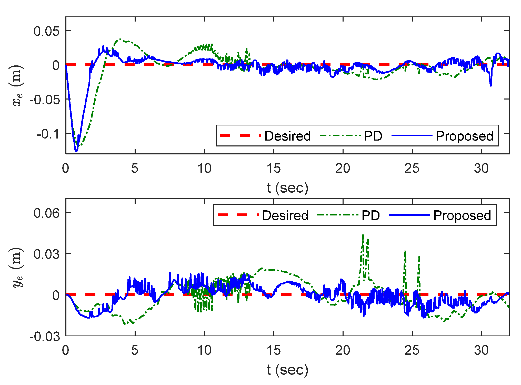
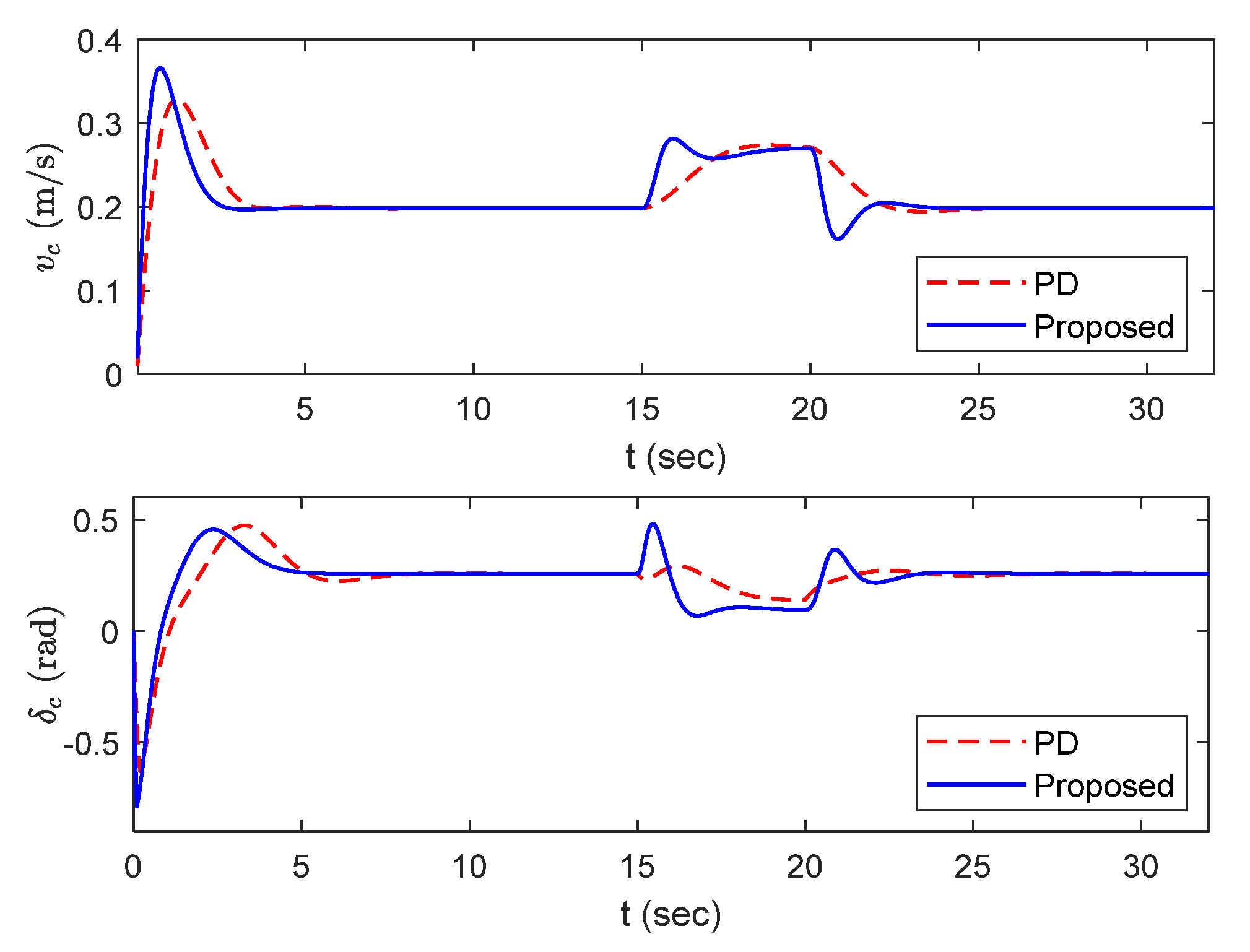
  • A backstepping controller is designed based on the estimated values to achieve better disturbance rejection performance of the CLMR. The effectiveness of the designed controller is verified by a simulation and experimentally.
The rest of this paper is as follows: Section 2 gives the problem formulation. Details of the design process of the linear ESO and backstepping controller are presented in Section 3. Section 4 shows the simulation and experimental results for the CLMR. Finally, Section 5 concludes this paper.
Remark 1.
Although research in this paper is mainly based on the kinematic model to accomplish the trajectory tracking task of CLMRs in low-speed scenarios, it also provides suggestions for whether to use the kinematic or dynamic model for the trajectory tracking task of a CLMR based on the above research from the following four perspectives:
  • Tracking accuracy: for application scenarios that do not require high accuracy, the kinematic model can be chosen; for scenarios that require higher control accuracy, the dynamic model is more appropriate.
  • Traveling speed: the kinematic model is suitable for low-speed scenarios (speed less than 5 m/s), while the dynamic model is more suitable for high-speed scenarios [16].
  • Computing power: the kinematic model is relatively simple and suitable for systems with limited computational power. The dynamic model is more complex and suitable for computationally powerful systems.
  • Sensor limitations: the kinematic model usually requires only position and velocity sensors, while dynamic models also require acceleration sensors.

2. Problem Formulation

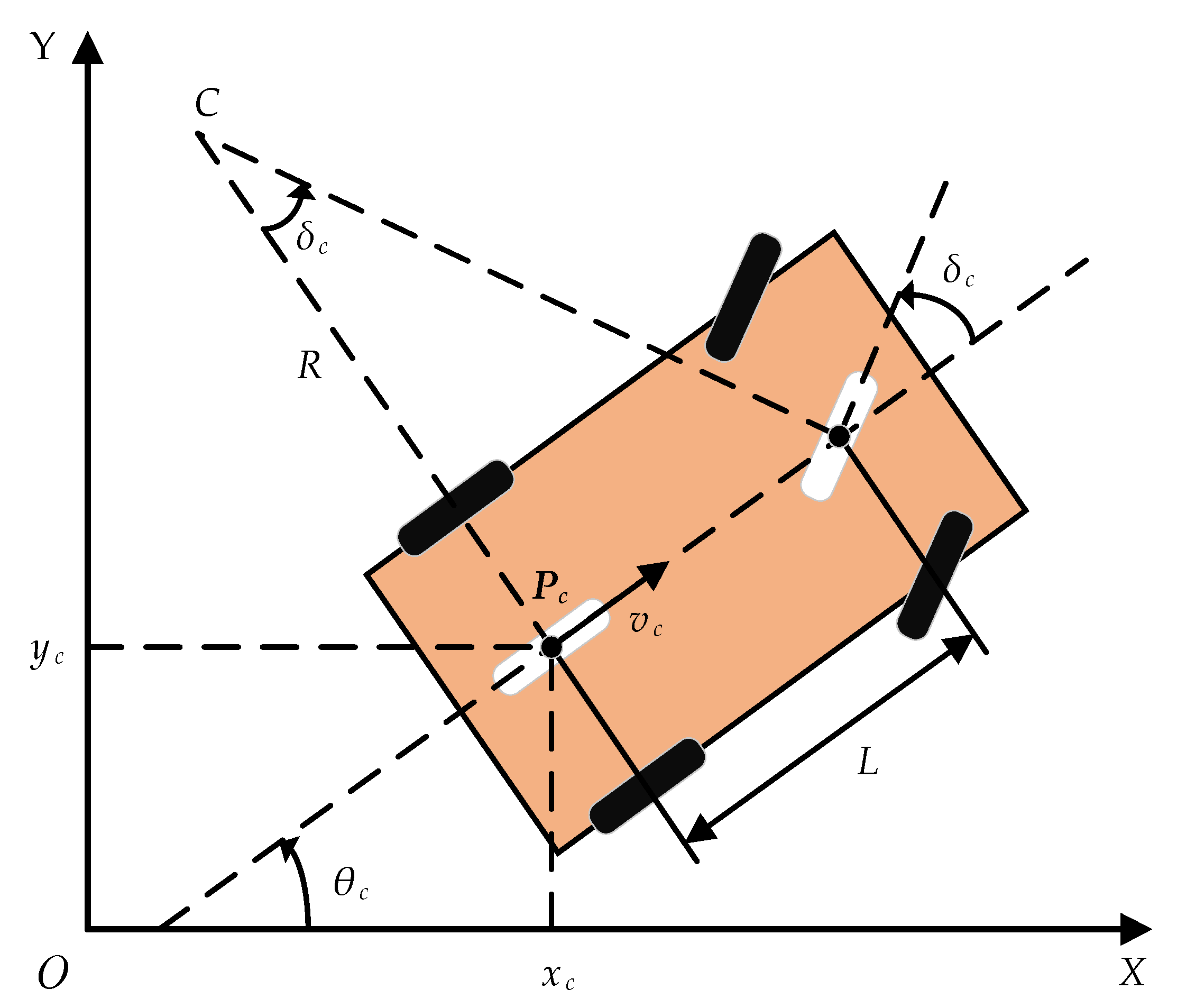
2.1. Kinematic Model with Disturbances

An ideal kinematic model of a CLMR moving on a planar surface is shown in Figure 1. In Figure 1, the front and rear wheels of the CLMR are lumped together such that the rear wheel is used as the drive, and the front wheel is used for steering. The CLMR is in the global coordinate system  { X O Y } . The state of motion of the CLMR can be represented by
P c = [ x c y c θ c ] T
where  ( x c , y c )  is the position coordinate of the rear wheel, and  θ c  indicates the yaw angle with respect to the  X  axis. Point  C  is the center of rotation of the CLMR, and  R  is its radius of rotation. Based on the above definition, the ideal kinematic model of CLMR is expressed by
{ x ˙ c = v c cos θ c y ˙ c = v c sin θ c θ ˙ c = v c / R = v c tan δ c / L
where  L  is the wheelbase of the CLMR, and  δ c  and  v c  are the steering angle of the front wheel and the forward speed of the CLMR.
Due to modeling errors and external disturbances that are usually present in trajectory tracking tasks for CLMRs, the kinematic controller designed based on Equation (2) will lead to the degradation of trajectory tracking accuracy. Therefore, modeling errors and external disturbances need to be introduced into the ideal kinematic model. The kinematic model of the CLMR with disturbances can be written as
{ x ˙ c = v c cos θ c + d x y ˙ c = v c sin θ c + d y θ ˙ c = ω c + d θ
where  w c  is the yaw angular velocity of the CLMR, and  d x d y , and  d θ  are the modeling errors and external disturbances of the CLMR in the longitudinal, lateral, and yaw directions, respectively [30]. Modeling errors and external disturbances include the parameter errors of the CLMR, sensor measurement errors, and ground friction.
Assumption 1.
d ˙ i ,  i = x , y , θ  is the derivative of  d i , and it is bounded by a positive scalar  d ¯ i , i.e.,  | d ˙ i | d ¯ i .

2.2. Output Transform

From the Equation (3), the kinematic model with disturbances is a coupled, underdriven, nonlinear system, which increases the difficulty of controller design. The kinematic model of the CLMR is considered differentially flat, and a set of output equations can be utilized to decouple the system [31]. The set of output equations for system (3) is selected as
{ x l = x c + l cos θ c y l = y c + l sin θ c
where  x l  and  y l  are the selected output variables, and  l  is an arbitrary nonzero constant. The derivative of Equation (4) is calculated as
{ x ˙ l = x ˙ c l θ ˙ c sin θ c y ˙ l = y ˙ c + l θ ˙ c cos θ c
Substituting Equation (3) into Equation (5), then we have
{ x ˙ l = v c cos θ c l ω c sin θ c + d x l d θ sin θ c y ˙ l = v c sin θ c + l ω c cos θ c + d y + l d θ cos θ c
To further obtain control of the CLMR at the level of acceleration, the second-order derivatives of the output variables are required. After taking the time derivative of  x ˙ l  and  y ˙ l , the following two-input, two-output disturbance system can be obtained:
{ x ¨ l = a 1 cos θ c a 2 l sin θ c + f k 1 + f d 1 y ¨ l = a 1 sin θ c + a 2 l cos θ c + f k 2 + f d 2
{ f k 1 = v c ω c sin θ c l ω c 2 cos θ c f k 2 = v c ω c cos θ c l ω c 2 sin θ c
{ f d 1 = v c d θ sin θ c l ( 2 ω c + d θ ) d θ cos θ c + d ˙ x l d ˙ θ sin θ c f d 2 = v c d θ cos θ c l ( 2 ω c + d θ ) d θ sin θ c + d ˙ y + l d ˙ θ cos θ c
where  a 1  and  a 2  are the linear and angular accelerations of the CLMR,  f k 1  and  f k 2  are the known model functions, and  f k 1  and  f k 2  are the total disturbances. The errors between  ( x l , y l )  and the desired position are defined as
{ x e = x l x d y e = y l y d
where  x d  and  y d  are the longitudinal position and lateral position of the desired trajectory. According to Equations (7) and (10), the dynamic equations for longitudinal and lateral errors of CLMR can be written as
x ¨ e = u 1 + f k 1 + f d 1 x ¨ d
y ¨ e = u 2 + f k 2 + f d 2 y ¨ d
where  x ¨ d  and  y ¨ d  are the longitudinal and lateral accelerations of the desired trajectory, and  u 1  and  u 2  are virtual control inputs. The relationship between  ( a 1 , a 2 )  and  ( u 1 , u 2 )  can be expressed as
[ u 1 u 2 ] = [ cos θ c l sin θ c sin θ c l cos θ c ] [ a 1 a 2 ]

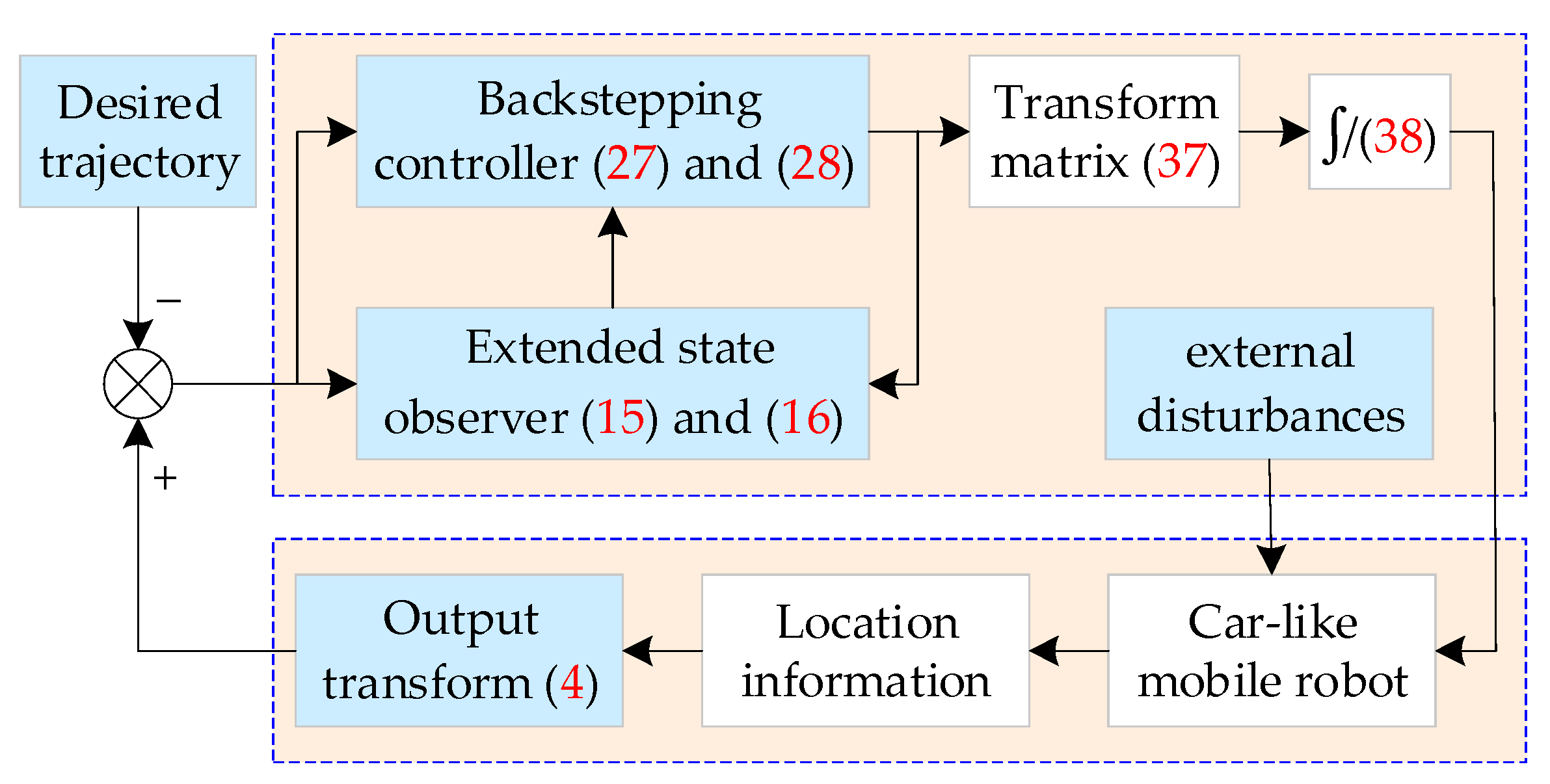
3. Trajectory Tracking Control Strategy

In this section, a trajectory tracking control strategy for the CLMR based on an ESO and backstepping control is proposed. The framework for the trajectory tracking task of the CLMR is depicted in Figure 2. The disturbances are estimated based on a linear ESO, and the trajectory tracking controller with disturbance compensation is designed using backstepping control. The details of the ESO and backstepping control will be discussed in the following section.

3.1. Extended State Observer

Since Equations (11) and (12) can be viewed as two second-order systems with the same form, Equation (11) can be chosen as an example for analysis.
Assumption 2.
( h 1 , h 2 )  is the derivative of  ( f d 1 , f d 2 ) , and it is bounded by the positive scalar ( h ¯ 1 , h ¯ 2 ) , i.e.,  | h 1 | h ¯ 1 ,  | h 2 | h ¯ 2 .
Let  f d 1  be the new state; then, Equation (11) can be rewritten as the following form:
{ x ˙ e 1 = x e 2 x ˙ e 2 = u 1 + f k 1 + x e 3 x ¨ d x ˙ e 3 = h 1
where  [ x e 1   x e 2   x e 3 ] T = [ x e   x ˙ e   f d 1 ] T  is the state of the system. For Equation (14), the ESO is designed as
{ z ˙ x 1 = l x 1 e x 1 + z x 2 z ˙ x 2 = l x 2 e x 1 + u 1 + f k 1 + z x 3 x ¨ d z ˙ x 3 = l x 3 e x 1
where  z x = [ z x 1   z x 2   z x 3 ] T  is the state of the ESO and  [ l x 1   l x 2   l x 3 ] T  is the observer gain.  e x 1 = x e 1 z x 1  is the estimation error of  x e 1 . Similarly, the ESO of Equation (12) can be written as
{ z ˙ y 1 = l y 1 e y 1 + z y 2 z ˙ y 2 = l y 2 e y 1 + u 2 + f k 2 + z y 3 y ¨ d z ˙ y 3 = l y 3 e y 1
where  z y = [ z y 1   z y 2   z y 3 ] T  is the state of the ESO and  [ l y 1   l y 2   l y 3 ] T  is the observer gain.  e y 1 = y e 1 z y 1  is the estimation error of  y e 1 = y e . From Equations (14) and (15), the estimation error of the ESO can be expressed as
{ e ˙ x 1 = e x 2 l x 1 e x 1 e ˙ x 2 = e x 3 l x 2 e x 1 e ˙ x 3 = l x 3 e x 1 + h 1
where  e x j = x e j z j j = 1 , 2 , 3  is the state of the estimation error. To simplify the proof process, Equation (17) can be rewritten in the following state space form:
e ˙ = A e + B h 1
where
A = [ l x 1 1 0 l x 2 0 1 l x 3 0 0 ] ,   B = [ 0 0 1 ]
Theorem 1.
For Equation (17), if selecting appropriate observer gains  [ l x 1   l x 2   l x 3 ] T  so that  A  is Hurwitz, The states of the estimation error will converge to the invariant set
Ω = { e | e T P e 4 h ¯ 1 2 B T P B λ max 2 ( P ) λ min 2 ( Q ) }
where  P  is the symmetric positive definite matrices, and  λ max ( )  and  λ min ( )  are the maximum and minimum eigenvalues of a matrix.
Proof. 
First, choose the Lyapunov function as
V 1 = e T P e
The derivative of  V 1  along Equation (18) is
V ˙ 1 = e ˙ T P e + e T P e ˙           = ( A e + B h 1 ) T P e + e T P ( A e + B h 1 )           = e T ( A T P + P A ) e + 2 h 1 e T P B
Since  A  is Hurwitz and  P  is a symmetric, positive, definite matrix, there exists a matrix  Q  satisfying  A T P + P A = Q . The matrices  P  and  Q  satisfy the following inequality
λ min ( P ) e T e e T P e λ max ( P ) e T e
λ min ( Q ) e T e e T Q e λ max ( Q ) e T e
According to Equations (21) and (22), it can be concluded that
e T Q e λ min ( Q ) λ max ( P ) e T P e
Furthermore,
2 h 1 e T P B 2 h ¯ 1 e T P B e T P B                 2 h ¯ 1 e T P e B T P B
According to Equations (23) and (24), V ˙ 1  can be derived as
V ˙ 1 = e T Q e + 2 h e T P B           λ min ( Q ) λ max ( P ) e T P e 1 + 2 h ¯ 1 e T P e B T P B           λ min ( Q ) λ max ( P ) e T P e ( e T P e 2 h ¯ 1 B T P B λ max ( P ) λ min ( Q ) )
It can be seen that  V ˙ 1 < 0  if  e T P e > 2 h ¯ 1 B T P B λ max ( P ) λ min ( Q ) . The states of the estimation error will converge to the invariant set  Ω . □

3.2. Backstepping Controller

This section takes Equation (11) as an example. Equation (11) can be rewritten in the following form:
{ x ˙ e 1 = x e 2 x ˙ e 2 = u 1 + f k 1 + f d 1 x ¨ d
where  [ x e 1   x e 2 ] T = [ x e   x ˙ e ] T . The goal of the trajectory tracking controller for the CLMR is to make the tracking error converge to zero. According to the Equation (26), the virtual control input  u 1  is designed as
u 1 = ( k x 2 ( x ˜ e 2 ) + f k 1 + z x 3 x ¨ d + x e 1 + k x 1 x ˙ e 1 )
where  x ˜ e 2 = x ˙ e 1 + k x 1 x e 1 . Similarly, the virtual control input  u 2  is designed as
u 2 = ( k y 2 ( y ˜ e 2 ) + f k 2 + z y 3 y ¨ d + y e 1 + k y 1 y ˙ e 1 )
where  [ y e 1   y e 2 ] T = [ y e   y ˙ e ] T  and  y ˜ e 2 = y ˙ e 1 + k y 1 y e 1 .
Theorem 2.
For Equation (27), disturbances in the system are estimated based on the linear ESO. When the control gains  k x 1 > 0  and  k x 2 > 0 , longitudinal errors  x e  converge to a sufficiently small range.
Proof. 
First, choose the Lyapunov function as
V 2 = x e 1 2 / 2
The derivative of  V 2  along  x e 1  is
V ˙ 2 = x e 1 x e 2
According to the idea of backstepping control, a virtual input is selected as
x e 2 = k x 1 x e 1
If the virtual input  x e 2 = x e 2 , Equation (30) can be rewritten as
V ˙ 2 = k x 1 x e 1 2
To ensure that  x e 2  can be tracked to  x e 2  accurately, define the error between  x e 2  and  x e 2  as
x ˜ e 2 = x e 2 x e 2
Define the new Lyapunov function as
V 3 = V 2 + x ˜ e 2 2 / 2
According to Equations (26) and (33), the derivative of  V 3  can be written as
  V ˙ 3 = x e 1 x ˙ e 1 + x ˜ e 2 x ˜ ˙ e 2           = x e 1 ( x ˜ e 2 + x e 2 ) + x ˜ e 2 ( x ˙ e 2 x ˙ e 2 )           = x e 1 ( x ˜ e 2 k x 1 x e 1 ) + x ˜ e 2 ( u 1 + f k 1 + f d 1 x ¨ d + k x 1 x ˙ e 1 )
Substituting Equation (27) into Equation (35),  V ˙ 3  can be derived as
V ˙ 3 = k x 1 x e 1 2 k x 2 x ˜ e 2 2 + x ˜ e 2 ( f d 1 z x 3 )           = k x 1 x e 1 2 k x 2 x ˜ e 2 2 + x ˜ e 2 e x 3
According to Theorem 1 under Assumption 2, the estimation error  e x 3  will converge to the invariant set. By choosing the appropriate observer gain, the invariant set will become sufficiently small. Then, we have  V ˙ 3 = k x 1 x e 1 2 k x 2 x ˜ e 2 2 0 . It can be seen that when  x e 1 0  and  x ˜ e 2 0 V 3 > 0 V ˙ 3 < 0 , according to the Lyapunov theorem of stability, longitudinal errors  x e  will converge to a sufficiently small range. □
Since  u 1  and  u 2  cannot be used as control signals for the CLMR, further processing is required. Based on the Equation (13), the linear acceleration  a 1  and angular acceleration  a 2  of the CLMR can be written as
[ a 1 a 2 ] = [ cos θ c sin θ c sin θ c / l cos θ c / l ] [ u 1 u 2 ]
The forward speed  v c  and yaw angular velocity  ω c  of the CLMR are obtained by integrating  a 1  and  a 2 . According to the Equation (2), the steering angle of the front wheel is calculated as
δ c = arctan ( L w c / v c )

4. Simulation and Experiment Results
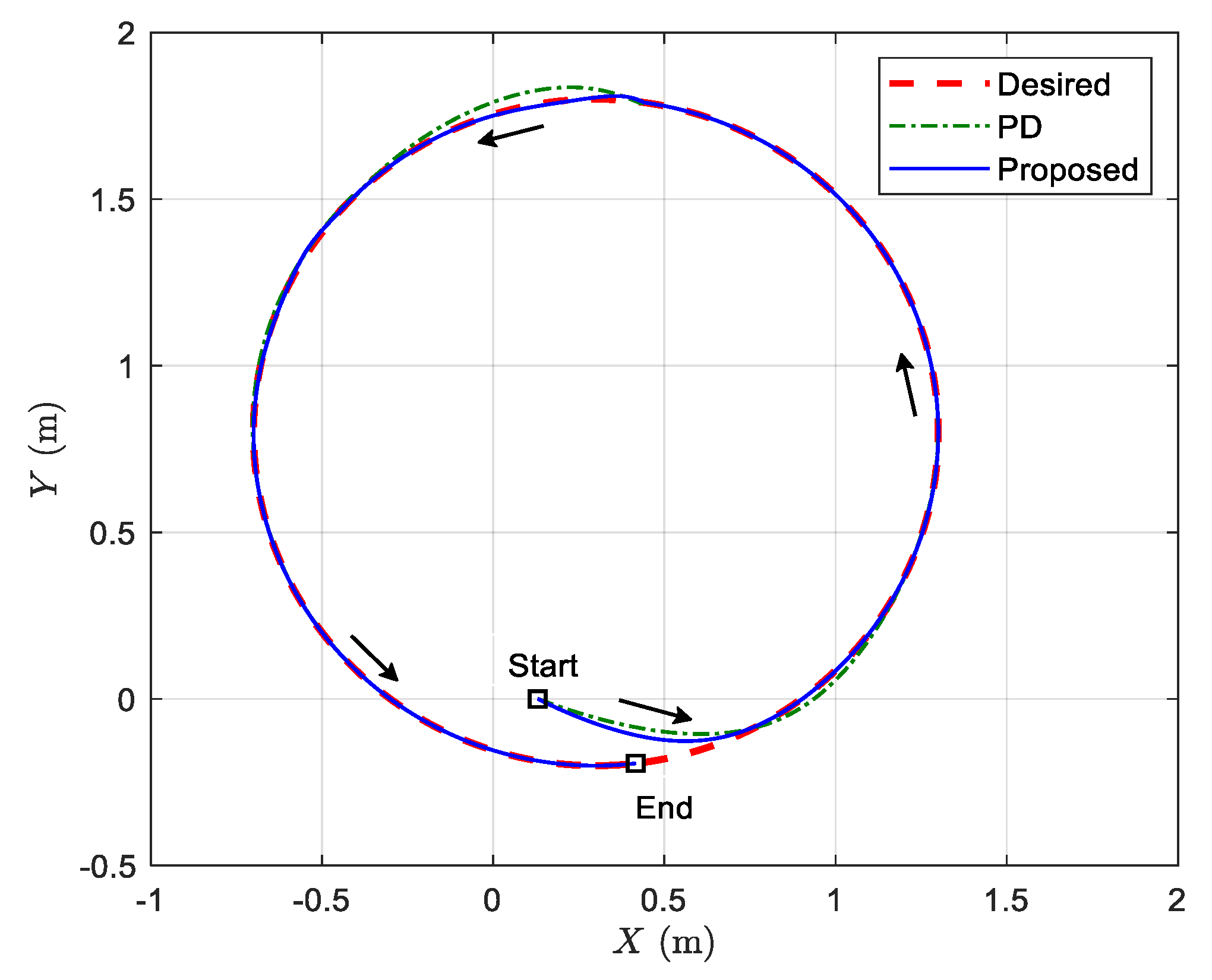
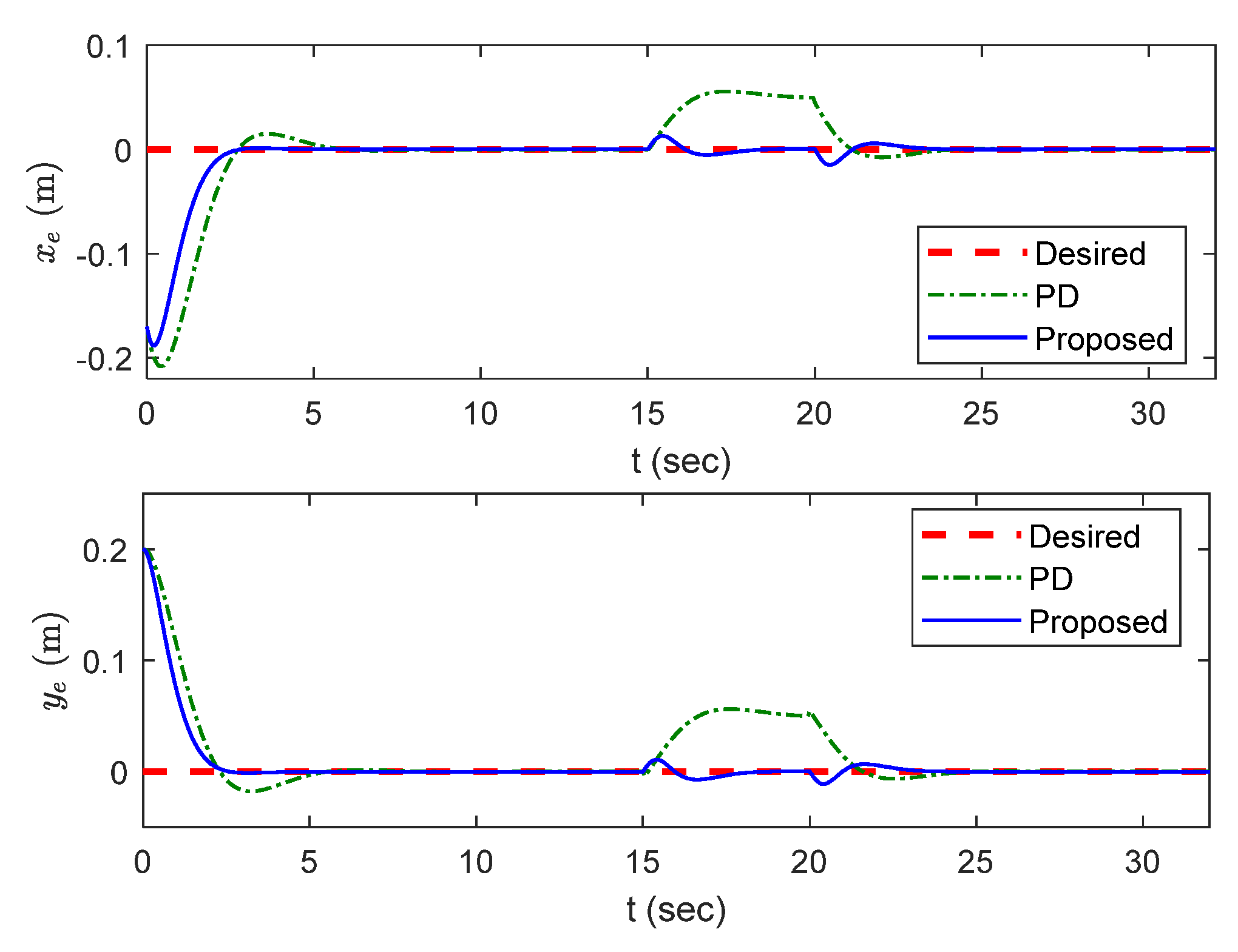
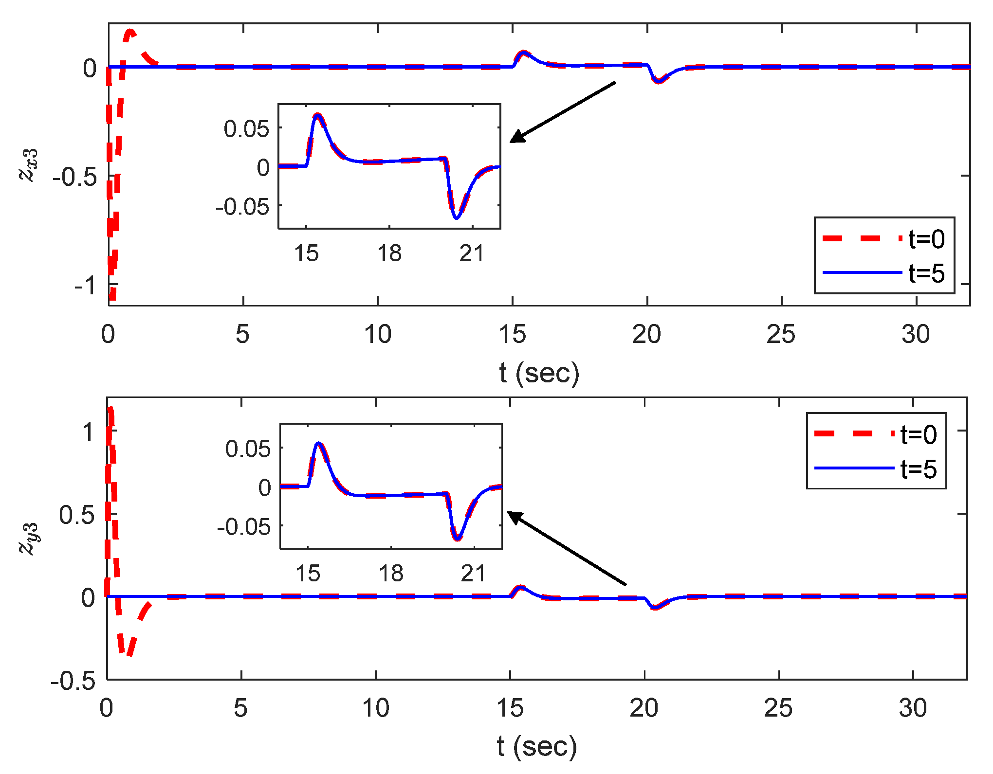
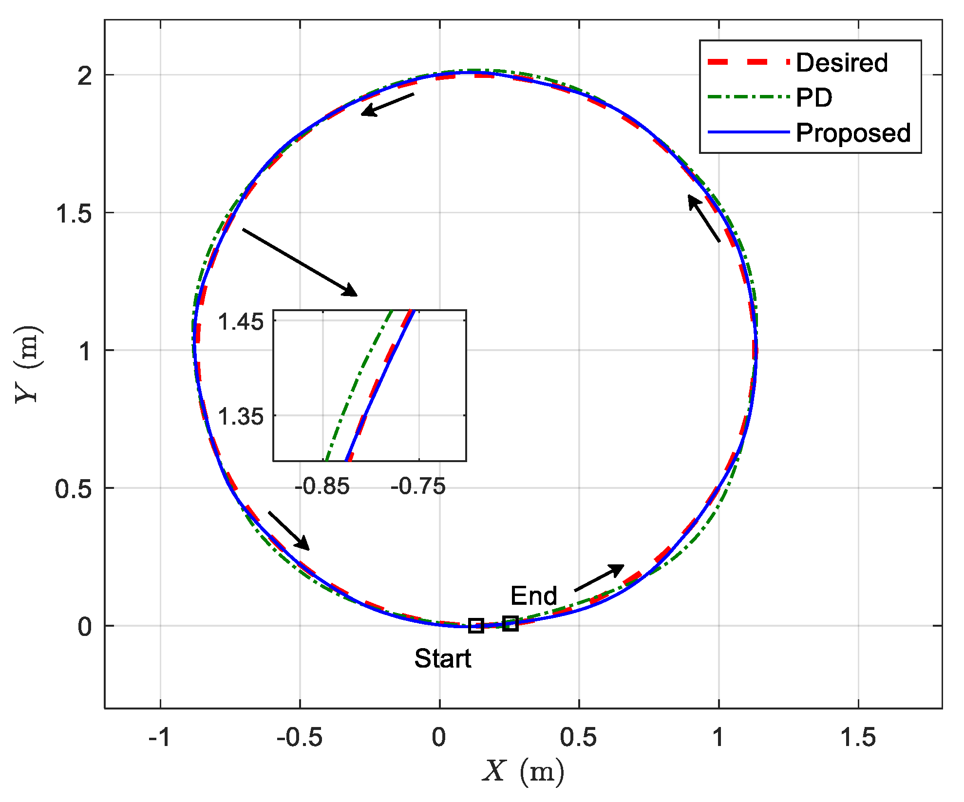
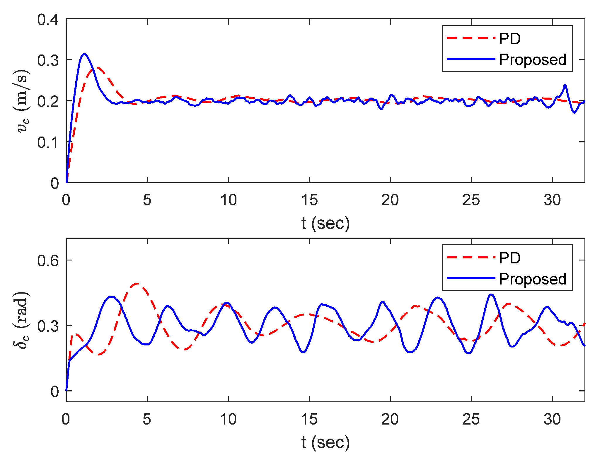
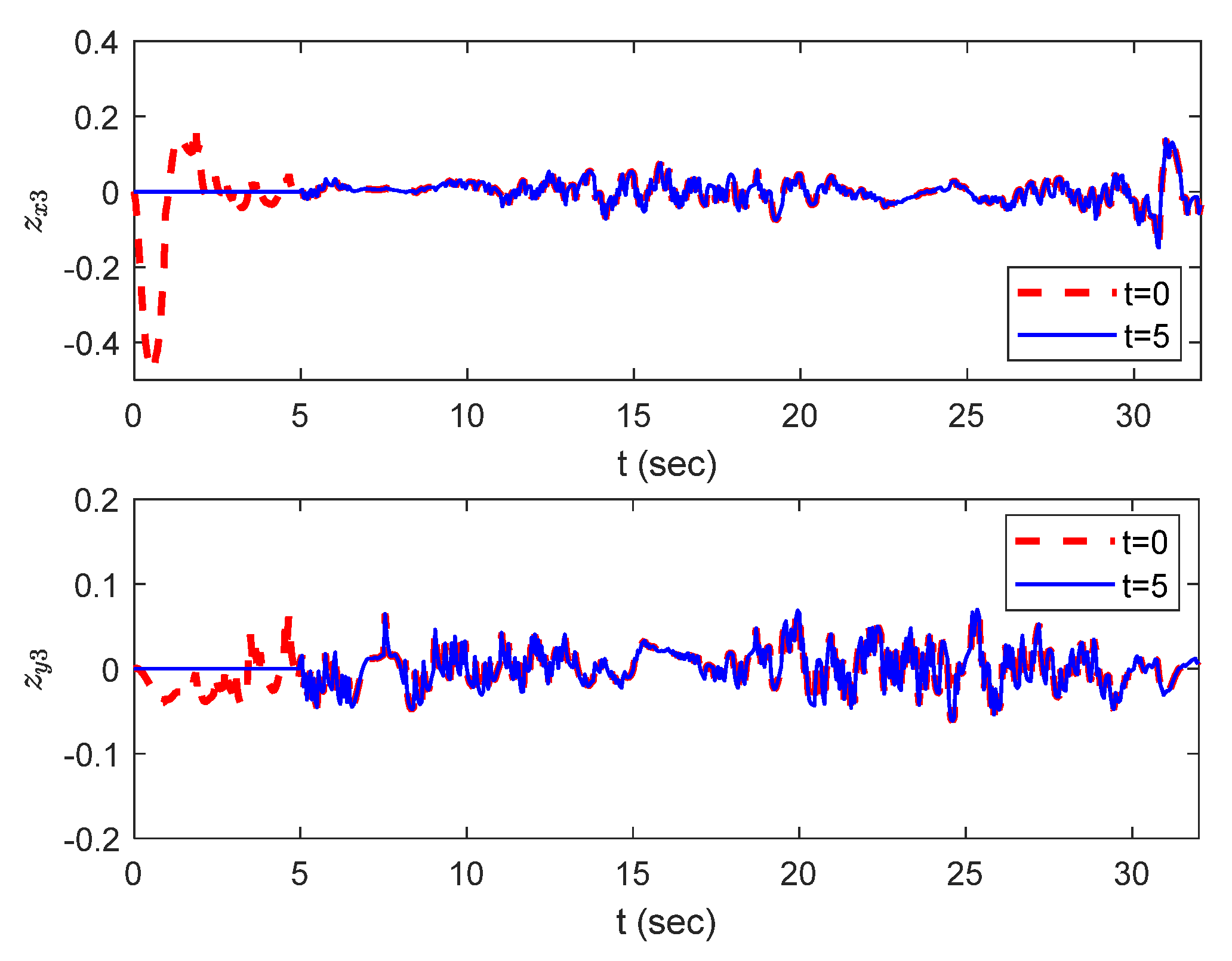
In this section, simulations and experiments are described to verify the effectiveness of the controller proposed in this paper. In the simulation, a circular trajectory is set as the reference trajectory, and the controller and models of the CLMR are constructed based on Matlab/Simulink. To further demonstrate the practicability of the designed controller, we conduct a real-world experiment on the Tianracer platform. For a comparison verification, the comparison controller is proposed based on Reference [20] (marked as PD). Both the controller proposed in this paper and the comparison controller are used to ensure that the center of the CLMR is able to track the desired trajectory. It should be mentioned that neither the experiment nor the simulation designed in this paper uses the estimates of the first 5 s of the ESO. The following simulation and experiment descriptions will give an explanation.

4.1. Simulation

In the simulation, the wheelbase of the CLMR is  L = 0.261  m, and the set up  l = L / 2  in Equation (4) is used to ensure that the center of the CLMR is tracking on the desired trajectory. The desired circular trajectory equation is written as
{ x d = cos ( 0.2 t + 1.5 π ) + 0.3 y d = sin ( 0.2 t + 1.5 π ) + 0.8
Since the simulation is performed under ideal conditions, external disturbances need to be added artificially during trajectory tracking to verify the effectiveness of the control scheme. In this section, the following disturbances are applied between 15 and 20 s during trajectory tracking  d x = d y = d θ = 0.05 . The main idea of the proposed scheme is to consider sudden, non-modeled disturbances in the system as total disturbances which are first estimated in real-time based on the ESO and subsequently compensated in the controller, thus improving the trajectory tracking accuracy of the CLMR. To further validate the effectiveness of the controller designed in this paper, the observer estimates  ( z x 2 , z y 2 )  are used instead  ( x ˙ e 1 , y ˙ e 1 )  in the simulation. For fairness in simulation and experimental comparisons, both controllers are designed with the same control gain. The gains of the controller and observer proposed in this paper and the comparative literature are shown in Table 1.
The simulation results of the CLMR tracking a circular trajectory are shown in Figure 3. Although the task of trajectory tracking for the CLMR can be accomplished using the comparison controller, it can be seen that the controller designed in this paper is closer to the desired trajectory in the presence of external disturbances. The evolution curves of longitudinal error and lateral error during the trajectory tracking of the CLMR are plotted in Figure 4. As shown in Figure 4, both controllers are able to ensure that the longitudinal and lateral errors of the CLMR converge to zero by 5 s. However, during the period of 15 to 20 s in the presence of external disturbances, it can be clearly seen that the control scheme proposed in this paper has a much smaller longitudinal and lateral error. The above simulation results show that the control scheme proposed in this paper achieves better disturbance rejection performance by the CLMR.
The evolution curves of the control signal of the CLMR are given in Figure 5. The controller scheme designed in this paper has faster regulation in terms of the forward speed and the steering angle of the front wheel, which is the key to resisting external disturbances. The evolution curves of the external disturbance values estimated by the ESO are shown in Figure 6. In the initial phase, the disturbances estimated by the ESO show significant peaks, which is not conducive to the stabilization of the system. Therefore, in the initial phase, neither the experiment nor the simulation designed in this paper uses the values estimated by the ESO. The values estimated by the ESO during the disturbance are plotted in the localized, zoomed-in view in Figure 6.

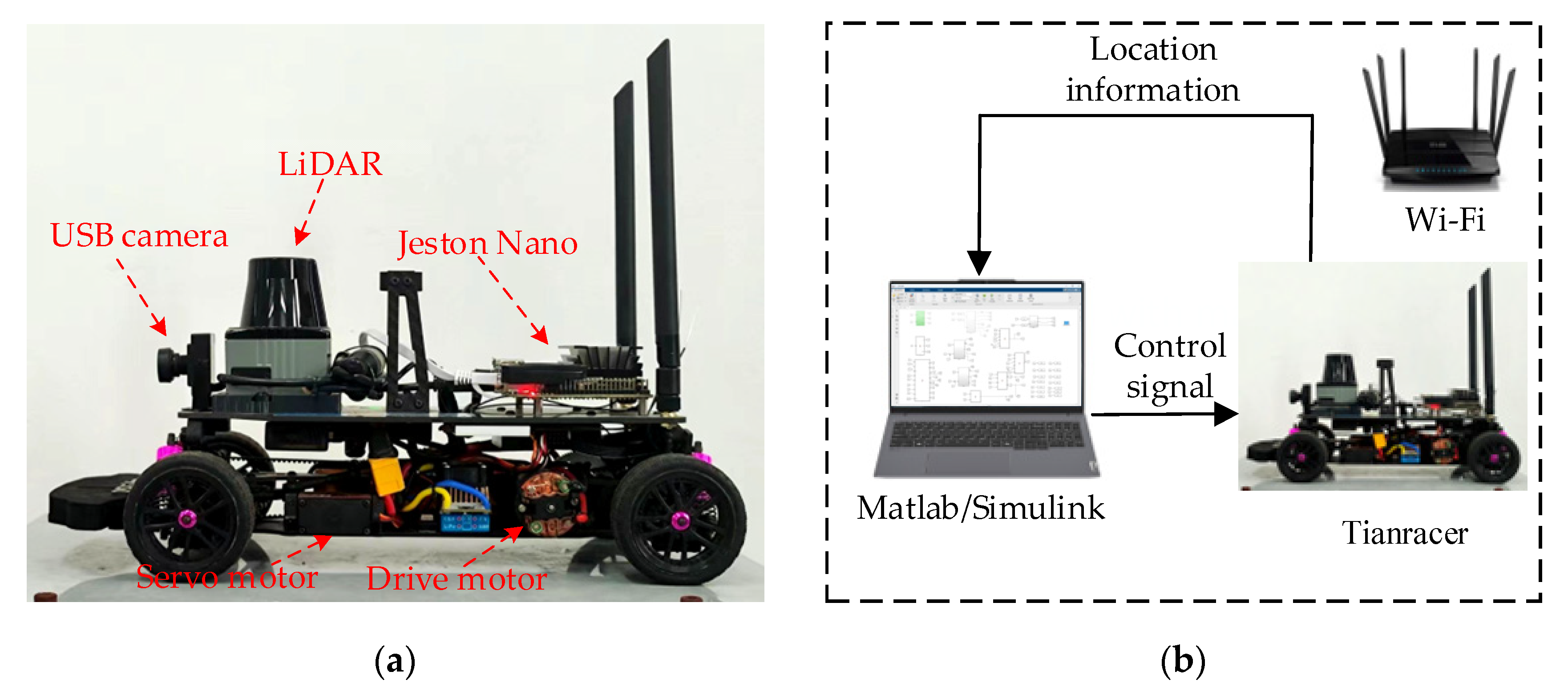
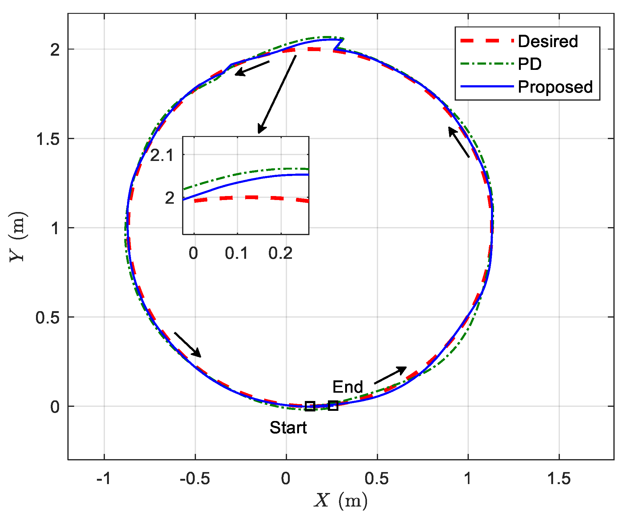
4.2. Real-World Experiment

To further validate the effectiveness of the designed controller in real-world scenarios, Tianracer was used as an experimental platform to accomplish the trajectory tracking task of the CLMR. The experimental scheme for the trajectory tracking of the CLMR is shown in Figure 7. As seen in Figure 7a, the NVIDIA Jetson Nano is used with Robot Operating System (ROS) as the onboard processor for Tianracer. The steering angle of the front wheel and the forward speed are controlled by servo and drive motors. Meanwhile, Tianracer also provides a wide range of sensors, including encoders, MPU6050, a USB camera, and single-beam LiDAR. The experimental step is shown in Figure 7b. Utilizing the distributed framework of ROS, Tianracer is used as a host, and a personal computer (PC) with Matlab/Simulink R2020a is used as a secondary device. Firstly, the signals from encoders and the MPU6050 are integrated for localization information. Then, the onboard processor sends the localization information to the PC, and the control signals are sent from the PC to the onboard processor to achieve closed-loop control. The transmission of signals between the onboard processor and the PC is accomplished through wireless Wi-Fi communication.
All the control methods were tested on an Intel i5-13500 CPU with 16 GB memory. Using Simulink to design the controller and communicating with the actual robot via ROS, can quickly validate the control scheme and facilitate subsequent iterative optimization. At the same time, Simulink supports the online generation of ROS code; through further debugging and optimization, ROS code generated based on Simulink can be deployed to resource-constrained systems (the NVIDIA Jetson Nano with ROS).
In the experiment, the wheelbase of the Tianracer is  L = 0.261  m, and the gains of the controller and observer are kept constant with the values set in the simulation. In the experiment, the friction of the ground, the noise of the sensor, and other factors are considered external disturbances. The redesigned desired trajectory is shown as
{ x d = cos ( 0.2 t + 1.5 π ) + 0.13 y d = sin ( 0.2 t + 1.5 π ) + 1
The experiment results of CLMR tracking on a circular trajectory are shown in Figure 8. Both controllers enable the CLMR to track the desired trajectory. As shown in the localized, zoomed-in view in Figure 8, the controller scheme designed in this paper makes the trajectory of the CLMR closer to the desired trajectory. The evolution curves of longitudinal error and lateral error during the trajectory tracking of the CLMR in this experiment are plotted in Figure 9. It can be clearly seen that the controller designed in this paper has smaller longitudinal and lateral errors throughout the trajectory tracking process. The trajectory tracking error further validates the effectiveness of the controller proposed in this paper.
The evolution curves of the control signals for the CLMR in the experiment are given in Figure 10. According to Figure 10, it can be seen that both controllers are able to track circular trajectories with a speed of 0.2 m/s. The evolution curves of the external disturbances estimated by the ESO in the experiment are plotted in Figure 11. In the initial phase of the experiment, the disturbance values estimated by the ESO are not used to avoid system instability caused by peak error. The experimental results show that the backstepping controller was designed based on estimated values to achieve better disturbance rejection performance of the CLMR.
In order to verify the effectiveness of the proposed control scheme in dealing with sudden non-modeled disturbances, disturbances are introduced during the trajectory tracking of the CLMR. Disturbances are assumed to be a measurement error of 0.05 m generated by the sensor during a period from 15 to 18 s. The results of the trajectory tracking of the CLMR during sudden disturbances are shown in Figure 12.
From Figure 12, it can be seen that CLMR will deviate from the desired trajectory under sudden disturbances, but due to the control scheme proposed in this paper considering the influence of disturbances, compared with the comparison controller, the control scheme proposed in this paper brings the CLMR closer to the desired trajectory under sudden disturbances. The evolution curves of the longitudinal errors and lateral errors of the CLMR under sudden disturbances are illustrated in Figure 13. The lateral error and longitudinal error of the CLMR become larger at 15 s due to sudden disturbances. However, it can be seen that the control scheme proposed in this paper has a smaller tracking error during the disturbance compared to the comparison controller.
The speeds of the desired trajectories for the above experiments are all 0.2 m/s. To verify that the proposed controller can be applied to diverse speed scenarios, the new desired trajectory can be written as
{ x d = 2 cos ( 0.2 t + 1.5 π ) + 0.13 y d = 2 sin ( 0.2 t + 1.5 π ) + 2
where the speed of the desired trajectory is 0.4 m/s. The experimental results of the CLMR tracking a circular trajectory at 0.4 m/s are presented in Figure 14. Both control schemes enable the CLMR to track the desired trajectory, but as shown in the localized, zoomed-in view in Figure 14, the controller scheme designed in this paper brings the trajectory of the CLMR closer to the desired trajectory. The evolution curves of the longitudinal and transverse errors during CLMR trajectory tracking at 0.4 m/s are shown in Figure 15. Based on the trajectory tracking controller proposed in this paper, the longitudinal error and transverse error of the output trajectory of the CLMR remain within 3 cm after 5 s. Meanwhile, the controller proposed in this paper causes the CLMR to have smaller tracking errors compared to the comparison controllers.

5. Conclusions

In this article, a trajectory tracking control scheme for a CLMR is proposed based on an ESO and backstepping control to solve the problem of trajectory tracking accuracy decreases caused by modeling errors and external disturbances. Firstly, a set of output equations is utilized to split a kinematic model of the CLMR with disturbances into two mutually independent subsystems. Then, modeling errors and external disturbances of the CLMR are estimated based on a linear ESO. Finally, a backstepping controller based on the values estimated by the ESO is designed to improve the disturbance rejection capability of the CLMR in trajectory tracking tasks. The effectiveness of the proposed control scheme in disturbance rejection is verified in a simulation and an experiment. The control scheme proposed in this paper is mainly for low-speed CLMRs, ignoring the effect of tire force on the system. When the CLMR is in a high-speed scenario, the steering system causes the tire deformation to become larger. In this case, the kinematic model can hardly accurately describe the motion characteristics of the CLMR, which will reduce the accuracy of trajectory tracking. In the future, we intend to design a trajectory tracking controller based on a dynamic model of a CLMR to improve the trajectory tracking accuracy of CLMRs in high-speed scenarios.

Author Contributions

Conceptualization, C.Z. (Changfu Zhu); methodology, C.Z. (Changfu Zhu); software, C.Z. (Changfu Zhu) and C.Z. (Chenyang Zhao); validation, C.Z. (Changfu Zhu) and B.L.; formal analysis, C.Z. (Changfu Zhu); investigation, C.Z. (Changfu Zhu), C.Z. (Chenyang Zhao), and Y.W.; resources, C.Z. (Changfu Zhu), B.L., and C.Z.(Chenyang Zhao); data curation, C.Z. (Changfu Zhu) and C.Z. (Chenyang Zhao); writing—original draft preparation, C.Z. (Changfu Zhu); writing—review and editing, C.Z. (Changfu Zhu), B.L. and C.Z. (Chenyang Zhao); visualization, C.Z. (Changfu Zhu) and Y.W.; supervision, B.L.; project administration, C.Z. (Changfu Zhu) and B.L.; funding acquisition, B.L. All authors have read and agreed to the published version of the manuscript.

Funding

This work is supported by the National Natural Science Foundation of China (grant numbers 61973234 and 62203326) and in part by the Tianjin Natural Science Foundation (grant number 20JCYBJC00180). The authors acknowledge the anonymous reviewers for their helpful comments on the manuscript.

Institutional Review Board Statement

Not applicable.

Informed Consent Statement

Not applicable.

Data Availability Statement

The data presented in this study are available on request from the corresponding author.

Acknowledgments

The authors would like to thank Tiangong University for technical support and all members of our team for their contribution to the car-like mobile robot experiments.

Conflicts of Interest

The authors declare no conflicts of interest.

References

  1. Rea, P.; Ottaviano, E. Design and development of an inspection robotic system for indoor applications. Robot. Comput.-Integr. Manuf. 2018, 49, 143–151. [Google Scholar] [CrossRef]
  2. Choi, B.; Lee, W.; Park, G.; Lee, Y.; Min, J.; Hong, S. Development and control of a military rescue robot for casualty extraction task. J. Field Robot. 2019, 36, 656–676. [Google Scholar] [CrossRef]
  3. Harik, E.H.; Guinand, F.; Geipel, J. A semi-autonomous multi-vehicle architecture for agricultural applications. Electronics 2023, 12, 3552. [Google Scholar] [CrossRef]
  4. Sousa, R.B.; Petry, M.R.; Costa, P.G.; Moreira, A.P. OptiOdom: A generic approach for odometry calibration of wheeled mobile robots. J. Intell. Robot. Syst. 2022, 105, 39. [Google Scholar] [CrossRef]
  5. Wen, L.C.; Liu, Y.; Li, H.L. CL-MAPF: Multi-agent path finding for car-like robots with kinematic and spatiotemporal constraints. Robot. Auton. Syst. 2022, 150, 103997. [Google Scholar] [CrossRef]
  6. Qin, Z.B.; Chen, L.; Hu, M.J.; Chen, X. A lateral and longitudinal dynamics control framework of autonomous vehicles based on multi-parameter joint estimation. IEEE Trans. Veh. Technol. 2022, 71, 5837–5852. [Google Scholar] [CrossRef]
  7. Wang, H.; Zuo, Z.; Wang, Y.; Yang, H.; Hu, C. Estimator-based turning control for unmanned ground vehicles: An anti-peak extended state observer approach. IEEE Trans. Veh. Technol. 2022, 71, 12489–12498. [Google Scholar] [CrossRef]
  8. Yan, K.; Ma, B. Global posture stabilization for the kinematic model of a rear-axle driven car-like mobile robot considering obstacle avoidance. IEEE Robot. Autom. Lett. 2023, 8, 5568–5575. [Google Scholar] [CrossRef]
  9. Yeh, Y.C.; Li, T.H.S.; Chen, C.Y. Adaptive fuzzy sliding-mode control of dynamic model based car-like mobile robot. Int. J. Fuzzy Syst. 2009, 11, 272–286. [Google Scholar]
  10. Li, P.; Yang, H.; Li, H.; Liang, S. Nonlinear ESO-based tracking control for warehouse mobile robots with detachable loads. Robot. Auton. Syst. 2022, 149, 103965. [Google Scholar] [CrossRef]
  11. Zhang, X.; Wang, R.; Fang, Y.; Li, B.; Ma, B. Acceleration-level pseudo-dynamic visual servoing of mobile robots with backstepping and dynamic surface control. IEEE Trans. Syst. Man Cybern. Syst. 2019, 49, 2071–2081. [Google Scholar] [CrossRef]
  12. Xu, S.; Peng, H. Design, analysis, and experiments of preview path tracking control for autonomous vehicles. IEEE Trans. Intell. Transp. Syst. 2020, 21, 48–58. [Google Scholar] [CrossRef]
  13. Ge, L.; Zhao, Y.; Ma, F.; Guo, K. Towards longitudinal and lateral coupling control of autonomous vehicles using offset free MPC. Control Eng. Pract. 2022, 121, 105074. [Google Scholar] [CrossRef]
  14. Wang, X.; Sun, W. Trajectory tracking of autonomous vehicle: A differential flatness approach with disturbance-observer-based control. IEEE Trans. Intell. Veh. 2023, 8, 1368–1379. [Google Scholar] [CrossRef]
  15. Kong, J.; Pfeiffer, M.; Schildbach, G.; Borrelli, F. Kinematic and dynamic vehicle models for autonomous driving control design. In Proceedings of the 2015 IEEE Intelligent Vehicles Symposium (IV), Seoul, Republic of Korea, 28 June–1 July 2015; pp. 1094–1099. [Google Scholar]
  16. Kebbati, Y.; Ait-Oufroukh, N.; Ichalal, D.; Vigneron, V. Lateral control for autonomous wheeled vehicles: A technical review. Asian J. Control 2023, 25, 2539–2563. [Google Scholar] [CrossRef]
  17. Rokonuzzaman, M.; Mohajer, N.; Nahavandi, S.; Mohamed, S. Review and performance evaluation of path tracking controllers of autonomous vehicles. IET Intell. Transp. Syst. 2021, 15, 646–670. [Google Scholar] [CrossRef]
  18. Hamerlain, F.; Floquet, T.; Perruquetti, W. Experimental tests of a sliding mode controller for trajectory tracking of a car-like mobile robot. Robotica 2014, 32, 63–76. [Google Scholar] [CrossRef]
  19. Pang, H.; Liu, N.; Hu, C.; Xu, Z. A practical trajectory tracking control of autonomous vehicles using linear time-varying MPC method. Proc. Inst. Mech. Eng. D J. Automob. Eng. 2021, 236, 709–723. [Google Scholar] [CrossRef]
  20. Dighe, Y.; Kim, Y.; Rajguru, S.; Turkar, Y.; Singh, T.; Dantu, K. Kinematics-only differential flatness based trajectory tracking for autonomous racing. In Proceedings of the 2023 IEEE/RSJ International Conference on Intelligent Robots and Systems (IROS), Detroit, MI, USA, 1–5 October 2023; pp. 1629–1636. [Google Scholar]
  21. Yagiz, N.; Hacioglu, Y. Backstepping control of a vehicle with active suspensions. Control Eng. Pract. 2008, 16, 1457–1467. [Google Scholar] [CrossRef]
  22. Qi, G.; Deng, J.; Li, X.; Yu, X. Compensation function observer-based model-compensation backstepping control and application in anti-inference of quadrotor UAV. Control Eng. Pract. 2023, 140, 105633. [Google Scholar] [CrossRef]
  23. Hu, J.; Zhang, Y.; Rakheja, S. Adaptive trajectory tracking for car-like vehicles with input constraints. IEEE Trans. Ind. Electron. 2022, 69, 2801–2810. [Google Scholar] [CrossRef]
  24. Rodríguez-Arellano, J.A.; Miranda-Colorado, R.; Aguilar, L.T.; Negrete-Villanueva, M.A. Trajectory tracking nonlinear H∞ controller for wheeled mobile robots with disturbances observer. ISA Trans. 2023, 142, 372–385. [Google Scholar] [CrossRef] [PubMed]
  25. Cui, R.; Chen, L.; Yang, C.; Chen, M. Extended state observer-based integral sliding mode control for an underwater robot with unknown disturbances and uncertain nonlinearities. IEEE Trans. Ind. Electron. 2017, 64, 6785–6795. [Google Scholar] [CrossRef]
  26. Han, J. From PID to active disturbance rejection control. IEEE Trans. Ind. Electron. 2009, 56, 900–906. [Google Scholar] [CrossRef]
  27. Gao, Z. Scaling and bandwidth-parameterization based controller tuning. In Proceedings of the 2003 American Control Conference(ACC), Denver, CO, USA, 4–6 June 2003; pp. 4989–4996. [Google Scholar]
  28. Wang, H.; Zuo, Z.; Wang, Y.; Yang, H.; Chang, S. Composite nonlinear extended state observer and its application to unmanned ground vehicles. Control Eng. Pract. 2021, 109, 104731. [Google Scholar] [CrossRef]
  29. Chang, S.; Wang, Y.; Zuo, Z.; Zhang, Z.; Yang, H. On fast finite-time extended state observer and its application to wheeled mobile robots. Nonlinear Dyn. 2022, 110, 1473–1485. [Google Scholar] [CrossRef]
  30. Lu, Q.; Chen, J.; Wang, Q.; Zhang, D.; Sun, M.; Su, C.-Y. Practical fixed-time trajectory tracking control of constrained wheeled mobile robots with kinematic disturbances. ISA Trans. 2022, 129, 273–286. [Google Scholar] [CrossRef]
  31. Tiriolo, C.; Lucia, W. On the design of control invariant regions for feedback linearized car-like vehicles. IEEE Control Syst. Lett. 2023, 7, 739–744. [Google Scholar] [CrossRef]
Figure 1. An ideal kinematic model of a CLMR moving on a planar surface.
Electronics 13 01563 g001
Figure 2. The framework for the trajectory tracking task of the CLMR.
Electronics 13 01563 g002
Figure 3. Simulation results of a CLMR tracking a circular trajectory.
Electronics 13 01563 g003
Figure 4. The evolution curves of longitudinal error and lateral error during CLMR trajectory tracking.
Electronics 13 01563 g004
Figure 5. The evolution curves of control signals for the CLMR.
Electronics 13 01563 g005
Figure 6. The evolution curves of external disturbances estimated by the ESO (dashed lines: output values of the ESO; solid lines: estimated values actually used by the controller).
Electronics 13 01563 g006
Figure 7. The experimental scheme for the trajectory tracking of the CLMR. (a) Experimental platform; (b) experimental step.
Electronics 13 01563 g007
Figure 8. The experiment results of the CLMR tracking a circular trajectory.
Electronics 13 01563 g008
Figure 9. The evolution curves of longitudinal error and lateral error during the trajectory tracking of the CLMR in the experiment.
Electronics 13 01563 g009
Figure 10. The evolution curves of control signals for the CLMR in the experiment.
Electronics 13 01563 g010
Figure 11. The evolution curves of external disturbances estimated by the ESO in the experiment (dashed lines: the output values of the ESO; solid lines: estimated values actually used by the controller).
Electronics 13 01563 g011
Figure 12. The experiment results of the trajectory tracking of the CLMR under sudden disturbances.
Electronics 13 01563 g012
Figure 13. The evolution curves of longitudinal error and lateral error during the trajectory tracking of the CLMR under sudden disturbances.
Electronics 13 01563 g013
Figure 14. The experimental results of the CLMR tracking a circular trajectory at 0.4 m/s.
Electronics 13 01563 g014
Figure 15. The evolution curves of longitudinal error and lateral error during the trajectory tracking of the CLMR at 0.4 m/s.
Electronics 13 01563 g015
Table 1. Parameters of controller and observer.
SchemesController ParametersObserver Parameters
PD k x 1 = k x 2 = 1.65
k y 1 = k y 2 = 1.65
no
Proposed k x 1 = k x 2 = 1.65
k y 1 = k y 2 = 1.65
l x 1 = 15 ,   l x 2 = 75 ,   l x 3 = 125
l y 1 = 15 ,   l y 2 = 75 ,   l y 3 = 125
Disclaimer/Publisher’s Note: The statements, opinions and data contained in all publications are solely those of the individual author(s) and contributor(s) and not of MDPI and/or the editor(s). MDPI and/or the editor(s) disclaim responsibility for any injury to people or property resulting from any ideas, methods, instructions or products referred to in the content.

