Abstract
Higher-order statistics investigate the phase relationships between frequency components, an aspect which cannot be treated using conventional spectral measures such as the power spectrum. Among the widely used higher-order statistics, the bispectrum ranks prominently. By delving into higher-order correlations, the bispectrum offers a means of extracting additional merits and insights from frequency coupling, enhancing our understanding of complex signal interactions. This analytical approach overcomes the limitations of traditional methods, providing a more comprehensive view of the complex relationships within the frequency domain. In this paper, the extensive use of the bispectrum in various scientific and technical areas is firstly emphasized by presenting very recent applications. The main scope of this work is to investigate the consequences of various non-linearities in the creation of phase couplings. Specifically, the quadratic, the cubic and the logarithmic non-linearities are examined. In addition, simple recommendations are given on how the underlying nonlinearity could be detected. The total approach is novel, considering the capability to distinguish from the bispectral content if two non-linearities are simultaneously present.
1. Introduction
Over the past decades, higher-order spectra (HOS) [1,2], also known as polyspectra, have earned recognition as a sophisticated mathematical and signal processing tool for nonlinear system analysis. It is acknowledged that the traditional power spectrum, defined as the Fourier transform of the autocorrelation sequence (the second-order cumulant), fails to provide information about the phase of the system’s frequency response and does not indicate any evidence of nonlinearity. This means that phase couplings between harmonics cannot be detected from the power spectrum of the signal, since it only provides information about the power of each harmonic it contains and not the relevant phases among the harmonics [1,2,3,4,5,6]. The HOS are defined as the multidimensional Fourier transform of higher order cumulants of a stationary random process, thereby overcoming the limitations of power spectra. The structure of HOS allows the deduction of various properties of signals that do not emerge when using the power spectrum alone. For instance, different signals can have the same correlation function or power spectrum, but they can be distinguished by employing HOS. Additionally, various signal processing methods using HOS are employed to address problems that cannot be resolved solely through second-order statistics. The bispectrum, a second-order HOS, serves as a useful tool for identifying processes that are either non-Gaussian or generated through non-linear mechanisms. The bi-coherence, a normalized version of the bispectrum, is extensively utilized as an index of the quadratic phase coupling degree in the signal of interest [1,2,3,4,5,6].
In addition to bispectrum and bi-coherence, other HOS measures, such as the trispectrum and higher-order cumulants, further extend the analysis capabilities for non-linear systems. These measures provide insights into the intricate relationships among different frequency components within a signal, offering a more comprehensive understanding of the underlying processes. Moreover, the application of HOS is not limited to signal analysis; it has found utility in diverse fields such as communications, radar and biomedical signal processing. The ability of HOS to capture non-linearities and non-Gaussian behavior makes them a valuable tool for uncovering hidden patterns and structures in complex data sets. Despite their advantages, the computational complexity associated with HOS has led to the development of efficient algorithms and techniques for their implementation. Ongoing research continues to explore novel applications and advancements in the use of higher-order spectra for a deeper understanding of complex systems and signals.
Bispectral analysis is an effective signal processing tool for investigating interactions between oscillations and has been adapted to the continuous wavelet transform for time-evolving analysis of open systems. In the work by Newman et al. [7], a suitable normalization of the wavelet bispectrum formula is provided that enables it to be treated as a density to be integrated.
The material cited in the following paragraphs highlights the great importance of the bispectrum in the analysis of many categories of signals. Accordingly, as it is well known, non-linearities play a crucial role in power system signals, serving as key indicators of various physical behaviors, including frequency interactions [1,2,3,4,5,6], inter-harmonic effects on power systems [6,8], incipient failures [2], noise cancellation [9] and phase coupling [3,4,9]. Traditional techniques for assessing rotating asymmetry, such as imbalance and bending shafts, have been proven effective in recent years [4,8,9,10,11,12]. However, these conventional methods often assume signal linearity and stationarity, limiting their applicability to diverse situations [13,14,15]. The underlying concept is that as power systems degrade, they tend to exhibit increased non-linearity, leading to the generation of new frequency components [16,17,18]. These new frequencies become phase-coupled with the original interaction frequencies, giving rise to what are known as non-linear interactions. The phase coupling correlation between the original interacting frequencies and the new frequency is recognized as quadratic phase coupling (QPC), serving as a real signature of non-linear interactions in dynamic systems [6,9,16,18]. Detecting QPC relationships in a signal is therefore a crucial element in understanding non-linear physical systems, particularly in the context of power generation.
Furthermore, other bispectral applications incorporate high voltage systems, fault signals, gear faults and other mechanical issues. Specifically, the work by Mitiche et al. [19] investigated the classification of insulation faults in a high voltage environment, based on real-world time-series signals labelled by condition monitoring experts. The proposed approach exploited the Bispectrum analysis and deep learning for feature extraction and classification. Grover and Turk [20] proved that deep convolutional neural networks, when trained on bispectrum images of fault signals using transfer learning, provide highly accurate and reliable results for fault diagnosis that are on par with the state-of-the-art results. A squeezed modulation signal bispectrum approach was developed by Xu et al. [21] to concentrate the leaked energy for accurately diagnosing gear faults with motor current signals. Bollineni et al. [22] developed a more refined method based on convolutional neural networks and the vibration bispectrum to increase the effectiveness and accuracy of fault diagnostics in bearings. The work in [23] proposes a novel multiple amplitude modulation and frequency modulation (AM–FM) demodulation method based on a local modulation signal bispectrum, which can demodulate the fault features of different components from the gearbox signal with multi-mesh frequency bands and multi-modulation components. The research by Hashempour et al. [24] introduced a novel algorithm so that Gaussian noises that appear in non-linear and unstable vibrations of motors are removed using wavelet decomposition, and non-linear noises are suppressed using the bispectrum method. Bispectrum analysis was employed in [25] to study the non-linear dynamic characteristics of a beam structure containing a breathing crack, from the perspective of numerical simulation and experimental validation. The use of higher-order spectral analysis, especially bispectrum and trispectrum analysis, for fault detection is gaining importance in recent studies due to the many advantages of HOS [26].
Additionally, Zhu and Li [27] applied the high-order cumulant spectrum and deep convolutional neural networks to feature the extraction and classification of aircraft target radar echoes. Liu et al. proposed [28] the utilization of the bispectral slice approach for the accurate recognition of complex UAV radar signals. A recent work [29] presented the coupling of frequencies corresponding to planets’ orbital signatures on the sunspot time series. The bispectrum was proven to be a unique tool to identify couplings of periodic phenomena on the surface of the sun.
The application of the bispectrum has gained popularity in biological systems, driven by the prevalent non-linear characteristics inherent in biological mechanisms. Notably, one such characteristic is the existence of non-linear interactions, which have been identified in neural [30,31], renal [32,33] and cardiovascular [34,35] systems. In the realm of neural system studies, the detection of non-linear interactions has proven particularly valuable. The bispectrum has effectively elucidated changes in interactions related to the levels of anesthesia and sedation [36]. Moreover, it has been employed in attempts to detect and predict epileptic seizure events [37]. The widespread adoption of the bispectrum in diverse biological studies underscores its versatility and effectiveness in uncovering non-linear interactions, making it a valuable analytical tool for researchers exploring the intricacies of biological systems. A study by Liu et al. [38] was on the foundation of the bispectrum approach for feature selection and employed the Vision Transformer model to achieve an automatic classification of normal and abnormal heart sound signals. Wang et al. [39] proposed the use of bispectrum analysis energy feature maps with frequency subdivision to be applied to breast cancer detection.
A novel parametrized multi-synchrosqueezing transform method based on weighted least squares, the IMSST and the PTFA, namely, PMSST, was proposed in [40]. In the PMSST, the IMSST is designed to obtain the signal time-frequency representation with high-energy aggregation.
This work theoretically investigates specific non-linearities, the presence of which create specific harmonic couplings. Namely, the quadratic non-linearity, which has already been studied, is firstly elaborated. The second non-linearity is the cubic one, while the third is the logarithmic non-linearity. The position and the strength of the derived frequency couplings are thoroughly derived and graphically depicted. A combination of the non-linearities, e.g., the quadratic and the logarithmic non-linearities, is examined in terms of the frequency couplings they generate. Finally, a procedure is outlined which helps to recognize the type of non-linearity present in a specific problem or even the simultaneous presence of two non-linearities.
By systematically investigating quadratic, cubic and logarithmic non-linearities, this study aimed to uncover their unique contributions to harmonic couplings. The theoretical analysis involves a detailed examination of the positions and strengths of the resulting frequency couplings, providing a comprehensive picture of the non-linear interactions within the system. This exploration extends to combinations of non-linearities, specifically focusing on the interplay between quadratic and logarithmic components.
This paper is organized as follows: In Section 2, the theory of high-order spectral statistics is presented. In Section 3, the position of coupled frequencies is analyzed based on the bispectrum representation. The quadratic non-linearity and its effect on frequency coupling is presented in Section 4, while in Section 5 the generation of coupled frequencies using a cubic non-linearity is provided. In Section 6, the logarithmic non-linearity is examined as far as the creation of coupled frequencies is concerned. The combination of two non-linearities, namely, quadratic and logarithmic non-linearities, is examined in Section 7 along with comments on the derived frequency couplings. In the same section, a discussion follows on the possibility to reveal the existing non-linearities from the derived couplings. The conclusions are drawn in Section 8.
2. Higher-Order Statistics Analysis
2.1. Higher-Order Moments
In the realm of probability and statistics, a fundamental concept involves the central moment of , the order for a random variable . This moment is precisely defined as the expected value of the nth power of the deviation between the random variable and its mean. The formulation encapsulating this definition is concisely presented in the following formula [1,2]:
where the notation represents the expected value operator and the superscript (n) indicates the order of the central moment. The probability density function of the random variable is denoted using . In this context, the mean value is specified as zero, and and denote the mean square value and the mean cube value, respectively, and so forth.
In the domain of higher-order statistics (HOS) signal analysis, the concept of moments extends to encompass moment functions, particularly correlation functions, related to a random process. For computational convenience, it is mathematically accepted that the random process possesses a zero mean. In practical scenarios, such as the analysis of stator current data from monitored electromechanical systems, the signal mean is initially computed and subtracted from the signal.
Expanding on the mathematical underpinnings of HOS analysis, various order correlation functions can be computed for the random process. The subsequent equation outlines these functions [1,2]:
where the superscript (*) denotes the complex conjugate. Specifically, the second-order correlation function corresponds to the well-known autocorrelation function. Extending further, the third-order correlation function is commonly referred to as the bi-correlation function. Similarly, the fourth-order correlation function is termed the tri-correlation, and so forth.
When considering linear signals and systems within the context of Equations (2) and (3), the focus is typically on a weakly stationary signal. However, delving into the interaction of three harmonic signals in a quadratic non-linear scenario, as will be discussed later, it is assumed that a random signal exhibits stability up to the third order, as expressed in Equations (4) and (5).
2.2. Power Spectrum
The Power Spectrum serves as a one-dimensional function of frequency and has proven highly effective in modeling linear physical problems. The discrete power spectrum is acquired through the Fourier transform (FT) of the autocorrelation function [1,2,41]. The estimation of the power spectrum can be expressed using the following equation:
where denotes the complex conjugate of and represents the discrete FT of the signal . It is crucial to note that the computation of the PS, as described, discards all information pertaining to phase. Consequently, this characteristic renders the PS unable to discern phase coupling (PC) signatures.
2.3. Bispectrum and Bi-Coherence
The bispectrum, derived from applying a two-dimensional Fourier transform to the third-order autocorrelation function , proves to be effective in identifying and quantifying quadratic phase coupling (QPC) [1,2,41]. Additionally, the bispectrum functions as a means to elucidate statistical associations among various frequency components within a signal. The formal definition is as follows [1]:
In order for the bispectrum to exhibit non-zero values at frequencies , it is necessary that the Fourier transforms at the individual frequency components , and are non-zero. Additionally, these three spectral components must display a correlation. It is crucial to emphasize that during the expectation process the bispectrum becomes zero due to phase randomization. However, when the phases are coupled, this is not the case. Unlike the power spectrum, the bispectrum is a complex quantity even when the signal is real-valued.
The symmetric regions of the bispectrum are depicted in Figure 1 [1,2,41]. Consequently, the analysis typically concentrates on a single non-redundant region. In this paper, the notation is utilized to denote the bispectrum in the non-redundant triangular region shown in blue in Figure 1. It is defined as , where is the sampling frequency. Additional information about the computational regions can be found in [1,2].
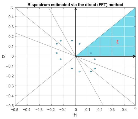
Figure 1.
The symmetrical structure of the bispectrum. The blue region is actually the appropriate space to investigate and recognize the frequencies’ coordinates that contribute to the formation of coupled components, where the region is .
The bispectrum proves to be highly useful in effectively addressing practical problems, as exemplified by the following examples [18,42,43]:
- For a stationary zero-mean Gaussian process , its bispectrum consistently remains zero.
- In contrast to the power spectrum, which discards phase information, the bispectrum retains it.
The bispectrum, serving as a quantified expression of higher-order statistics (HOS), represents the Fourier transform of the third-order cumulant or moment. Non-linearity influences these cumulants, and the bispectrum captures such effects. The estimated bispectrum is defined as
The expectation operation is crucial in this context, especially in QPC detection. It involves “ensemble averaging” for estimation: if phases are random, the bispectrum tends to zero, but if phases are coupled, it does not.
The diagonal slice of the bispectrum is a one-dimensional representation obtained by setting f1 = f2. This measure is defined as [4,8,9]
The bi-coherence, represented as the normalized bispectrum in Equation (10), functions as a metric that quantifies the degree of QPC within a signal or between frequency components of two signals. As bi-coherence is obtained through a normalization procedure, it does not give the energy coupled at the specific position but it just points out the position of the couplings. As mentioned earlier, QPC involves estimating the energy in all possible pairs of frequency components, denoted as and in accordance with the QPC definition, that is, the phase of the component at (where ) equals the sum of the phases of and [43,44]:
When the analyzed signal displays an arbitrary structure, the presence of PC can be expected.
3. Bispectrum of Coupled Frequencies
Addition:
Consider three signals, and where . The phase of signal arises from the sum of the phases of signals and , indicating an expected coupling edge at the coordinates . For instance, if and (Figure 2), a coupling edge is anticipated at coordinates (Refer to Figure 3).
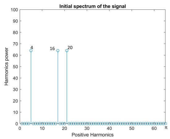
Figure 2.
The three harmonics power that appear at the 4th, 16th and 20th positions (dc corresponds to zero frequency component and is located at position 1). From the power spectrum it is not possible to distinguish that the 20th harmonic is the result of coupling the other two.
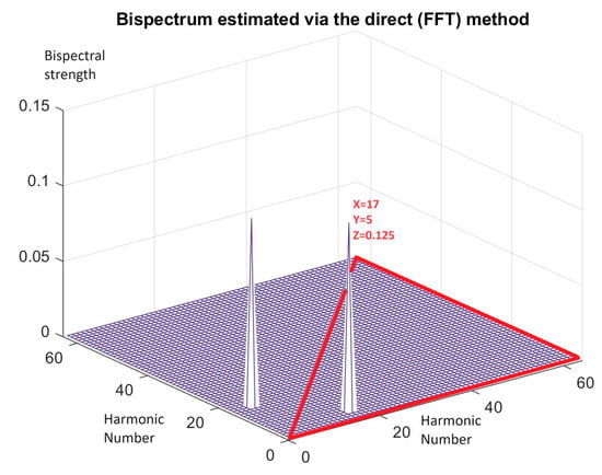
Figure 3.
Since (1, 1) is the position for dc, the coupling edge is present at coordinates i.e., for 4th and 16th coupled frequencies. The created 20th harmonic does not give any footprint in the region of the bispectrum which is enclosed in the red line. The red line includes the non redundant region of the bispectrum.
Subtraction:
Consider three signals, and , where . The phase of the signal results from the subtraction of the phases of signals and , suggesting there will be a coupling edge at the coordinates . For example, if and (Figure 4), a coupling edge is expected at coordinates (See Figure 5).
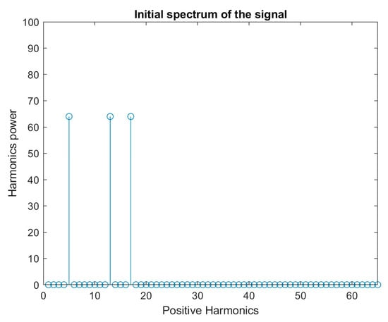
Figure 4.
The three harmonics power that appear at 4th, 12th and 16th positions (dc is at position 1). From the power spectrum it is not possible to distinguish which is the coupled harmonic.
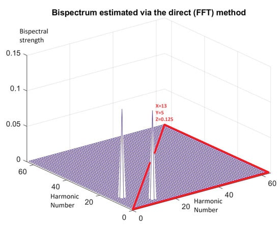
Figure 5.
Since (1, 1) is the position for dc, the coupling edge is present at coordinates , i.e., for 4th and 12th coupled frequencies. The original 16th harmonic does not give any footprint in the region of the bispectrum which is enclosed in the red line. The red line includes the non redundant region of the bispectrum.
It is worth noting that in the case of subtraction, the result aligns with the case of adding signals and . In other words, if the signals are and initially, where , and the phase of the signal can be derived by adding the phases of signals and , then a coupling edge is expected at the coordinates .
In summary, for three signals where one has a phase resulting from the addition or subtraction of the phases of the other two, coupling edges will occur at the coordinates corresponding to the two smallest phases of these signals.
In the field of signal processing, the phenomenon of coupling edges, as described in the context of signal addition and subtraction, highlights the complex relationships between signal phases. When signals and are combined to yield , the coupling edge appears at specific coordinates, revealing a harmonic interaction between frequencies and . This coupling effect, visualized in Figure 3, provides information on the synchronization of the signal phases.
Conversely, in the signal subtraction scenario, where phase results from the differentiated interaction between and , the resulting coupling edge is realized in coordinates determined by . This complex dance of frequencies, exemplified in Figure 5, shows the delicate balance required to de-phase the signal to yield a coherent result.
Moreover, the interesting statement, that in the case of signal subtraction the results mirror those of signal addition, highlights the symmetric nature of these signal functions. This symmetric behavior, enclosed by coupling edges at fixed coordinates, speaks to the underlying mathematical elegance that governs signal interactions.
It is important to note that these observations extend to three-signal scenarios, where the phase relationships are more complex. In cases where the phase of one signal is obtained by adding or subtracting the phases of two other signals, the coupling ends appear fixed at coordinates corresponding to the two smaller phases. This generalization adds a level of universality to the coupling phenomenon, demonstrating its applicability to various signal processing scenarios.
In conclusion, exploring the coupling edges in signal processing reveals a rich tapestry of relationships where the addition or subtraction of signal phases orchestrates complex patterns at specific frequency coordinates. These insights not only deepen our understanding of signal behavior, but also open avenues for further exploration in the colorful field of signal processing.
4. Bispectrum at the Output of Quadratic Non-linearities
4.1. Two Sinusoids as Input to the Qundratic System without dc Component
Consider three signals, and , where . The analysis of signal reveals its derivation from the square of the sum of the other two signals, and . Therefore, signal is calculated as
The anticipated coupling edges in the phase pairs, as elucidated in Section 3 are expected to manifest through the addition or subtraction of signals. Specifically, these coupling edges are predicted to occur at coordinates and (.
The above mathematical representation highlights a remarkable relationship between the three signals, , and . Signal is complexly constructed as the square of the sum of and . The distribution of the expression presents a combination of quadratic terms involving the cosine functions and . This formulation emphasizes the interplay of frequencies and phases in the composition of .
The synergy of and in introduces interesting dynamics, where the sum of their squares contributes to the complex pattern observed in . Visually, this can be seen as the constructive interference of the individual signals, resulting in a new signal with a distinct frequency and amplitude profile.
To illustrate (see Figure 6), let us consider the example where and :
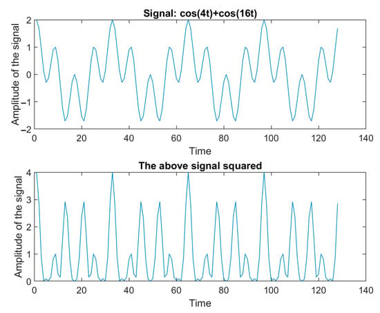
Figure 6.
Above: A composite signal of two harmonics with frequencies and . Bellow: The same signal squared according to Equation (12). The parameter “Time” in the horizontal axis is normalized to the sampling period of the digital system used.
The coordinates for the expected coupling edge resulting from the sum of the square of signals are and . These coordinates represent the phase pairs where coupling edges are anticipated, showcasing the intricate relationships among the signals and their frequencies.
A detailed explanation further clarifies the intricacies of coupling edges at the specified coordinates (12, 20) and (8, 12) in the context of signal phases. According to the principles described in Section 3, the occurrence of coupling edges at (12, 20) is evidenced by the generation of signals whose phases are aligned with the values 12 and 20.
For the coupling edge at (12, 20), a signal with the phase generated from the signals and is indentified, exemplifying the intricate interplay between these signals’ components.
Likewise, the coupling edge at (8, 12) is attributed to the signal , whose phase can be derived from the signals and . This specific combination of signal phases contributes to the formation of a coupling edge at the specified coordinates. These results are illustrated in Figure 7.
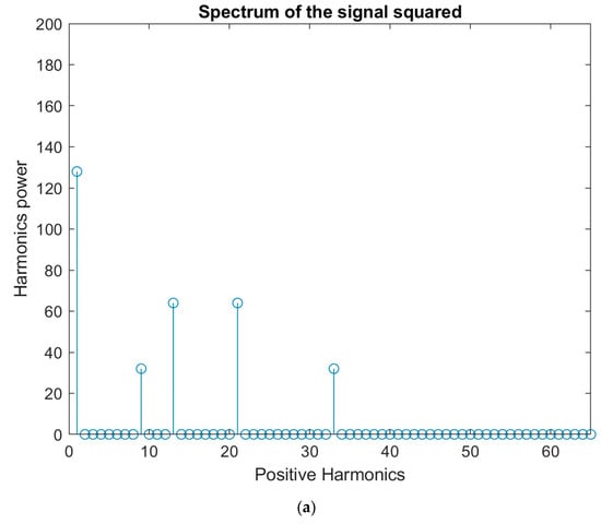
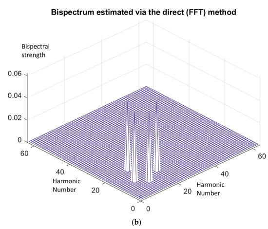
Figure 7.
(a) Harmonics power derived after passing two sinusoids with frequencies and through a quadratic non-linearity. No dc is present at the input of the non-linearity. (b) Two peaks are derived in the bispectral representation at positions (20, 12) and (12, 8) with equal strength, when the two sinusoids pass through a quadratic non-linearity.
The emphasis on the unique nature of these combinations, substantiated by the principles outlined in Section 3, reinforces the understanding that such coupling edges are intricately linked to specific phase relationships and cannot arise with alternative combinations, underscoring the precision and predictability that is inherent in the described signal.
A detailed example provides a concrete illustration of the principles discussed in Section 3, emphasizing the limitations and specific conditions under which coupling edges occur. Considering the signals and , the examination of their addition and subtraction sheds light on the resulting signal expansions:
- Addition scenario: The attempt to derive the signal resulting from the addition of and leads to an expansion that includes . However, this specific signal does not exist, highlighting the selective nature of coupling edges.
- Subtraction scenario: On the other hand, the subtraction of signals yields , a signal that indeed exists. According to the principles outlined in Section 3, a coupling edge is expected at coordinates (20, 12) in the case of subtraction. Importantly, the symmetry of the coordinates (12, 20) and (20, 12) indicates that no additional coupling edge was formed beyond the two mentioned, reinforcing the comprehensive understanding of coupling edge generation.
This analysis underscores the specificity and predictability associated with coupling edges, as they are intricately linked to the unique combinations and relationships among signal phases, as articulated in the preceding sections.
In practical terms, representing as a square of the sum of and has implications for signal analysis and processing. Understanding the complex nature of provides a basis for extracting meaningful information from complex signal structures, paving the way for applications in fields such as communications, signal processing and waveform analysis.
According to what has been exposed so far, a quadratic non-linearity was applied to a signal consisting of two equal-in-power sinusoids, and . The peaks in the bispectrum appear as they are presented in Table 1.

Table 1.
Bispectral coordinates for two equal-in-power sinusoids with frequencies and going through a quadratic non-linearity with .
4.2. Two Sinusoids as Input to the Quαdratic System with dc Component
Consider three signals, and , where . The 3rd signal, , is derived from the square of the sum of the other two signals ( and ) with the presence of the constant term 1, which introduces a dc component to the signal. This representation underscores the multifaceted composition of , encompassing both dc and the combined influence of the squared and . Expanding this expression, the following is obtained:
The anticipation of coupling edges, as elucidated in the previous sections, extends beyond the conventional coordinates and ( observed in scenarios without a dc component. In the presence of a dc component, additional coupling edges are expected to emerge at coordinates , (, and (. This diversity in coupling edges is attributed to the influence of the dc component, introducing distinct combinations of phases. Specifically, these coupling edges manifest at coordinates and (, where the combinations of these phases, when added together, result in combinations that exist in the signal’s development. The incorporation of a dc component thus contributes to a richer set of coupling edges, encompassing a variety of phase pairs that showcases the interplay between signals and the influence of the added constant term. The above results are presented in Figure 8 for the example and .
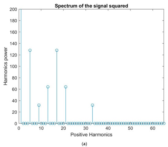
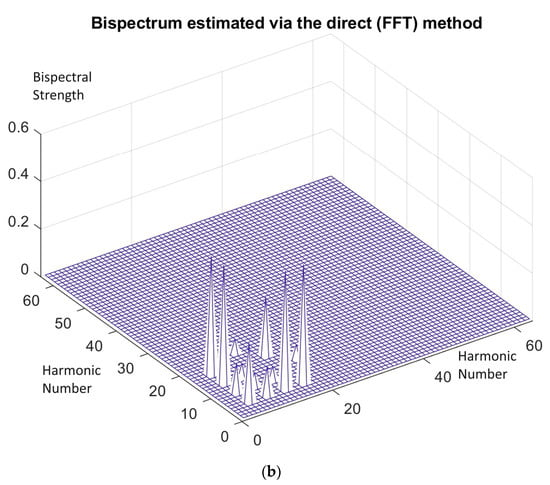
Figure 8.
(a) Harmonics power derived after passing two sinusoids with frequencies and including a dc component through a quadratic non-linearity. (b) With the presence of dc component, the two sinusoids derive many peaks in the bispectral representation when passed through a quadratic non-linearity, as explained in Section 4.2.
According to the above material, when a signal consisting of two sinusoids and of equal strength plus a dc component equal to 1 is going through a quadratic non-linearity, it presents a lot of bispectral peaks, which are given in Table 2.

Table 2.
Bispectral coordinates and at which bispectral peaks appear. They are given with respect to the two equal-in-power sinusoids and containing a dc term and going through a quadratic non-linearity (.
5. Bispectrum at the Output of Cubically Non-Linear System
Consider three signals, and , where . The representation in the bispectral space of signal reveals its derivation from the cube of the summation of the other two signals ( and ). Therefore, the signal is calculated as
The observations of the above relationships highlight a combination of scenarios involving both the square of the sum of two signals (as discussed in the previous section) and the presence of a dc component. Consequently, following the principles outlined in Section 2 and Section 3, the appearance of coupling edges in the phase pairs formed by their summation (or subtraction) from one or more of the other signals is expected.
The subsequent example in Figure 9 provides a concrete illustration with and .
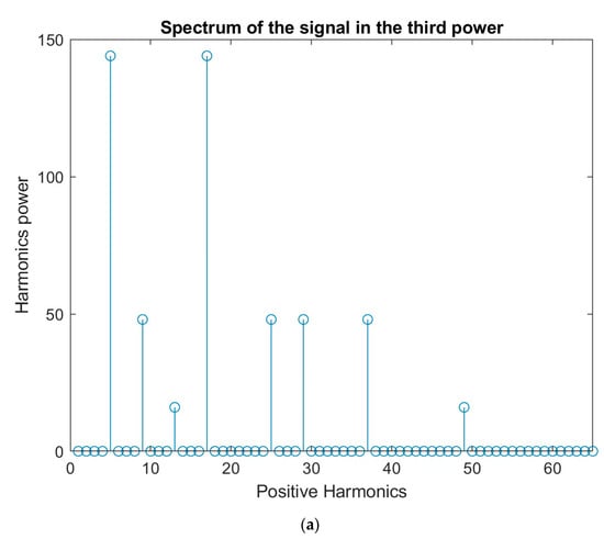
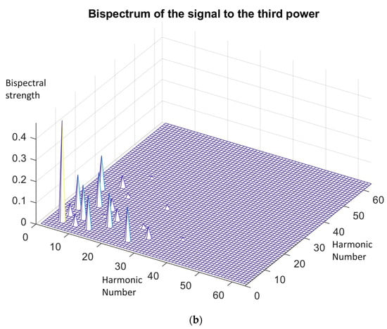
Figure 9.
(a) Harmonics power derived after passing two sinusoids with frequencies and without a dc component through a cubic non-linearity. (b) The two sinusoids derive many peaks in the bispectral representation when passed through a cubic non-linearity. Peaks with different strengths are present.
According to the above material, a signal consisting of two sinusoids and of equal strength, when going through a cubic non-linearity presents a lot of bispectral peaks, which are given in Table 3.

Table 3.
Bispectral coordinates for two equal-in-power sinusoids with frequencies and , with , going through a cubic non-linearity.
6. Bispectrum at the Output of a Logarithmic Non-Linear System
Finally, considering the case when the signal with and goes through a logarithmic transformation, where is selected so that the signal is always positive, a large variety of new frequency components appear, as shown in Figure 10a (in the example using and ). The produced peaks in the bispectrum cover all the available region in points that are additions or subtractions of and and their multiples. This result is depicted in Figure 10b.
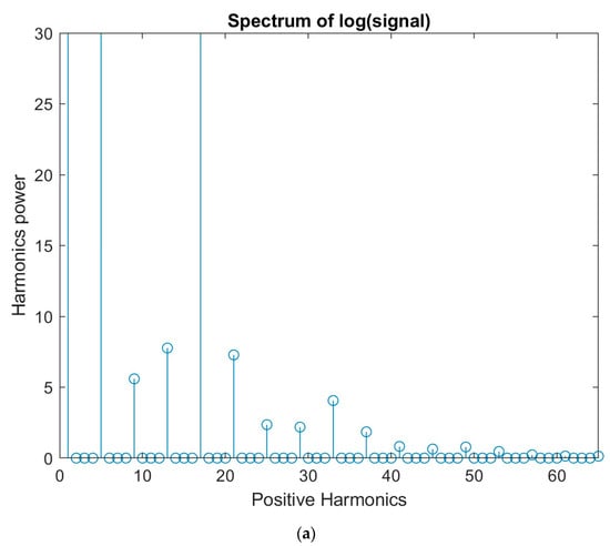
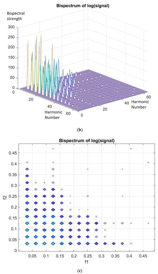
Figure 10.
(a) Harmonics power derived after passing two sinusoids with frequencies and through a logarithmic non-linearity. (b) The two sinusoids derive many peaks in the bispectral representation when passed through a logarithmic non-linearity. Peaks with different strengths are present. (c) The two sinusoids derive many peaks in the bispectral representation when are passed through a logarithmic non-linearity. Bispectral representation is depicted in carpet form which reveals that the bispectral energy covers like a textile the whole bispectral region of interest in points that are additions or subtraction of and and their multiples.
In order to be able to recover weak peaks at the output of the bispectral representation of the specific logarithmic non-linearity, a special preprocessing was applied. Explicitly, all the derived bispectral content was multiplied by 1000 so that all values became quite large, and much larger than 1, so that the weak peaks could be easily preserved as far as their strength has a comparable size to the strong peaks. For this specific case, in Figure 10c the same bispectral representation is depicted in carpet form, which reveals that the bispectral energy covers like a textile the whole bispectral region of interest in points that are additions or subtraction of and and their multiples.
7. Detecting Non-Linearities and Simultaneous Non-Linearities
According to the experimental results obtained in the previous sections, it is evident that the quadratic non-linearity gave a restricted number of bispectral peaks even if the original signal contains a dc component b and Figure 8b). These peaks appeared in positions where the largest of their coordinates at most being at the sum of the original frequencies. The same happened for the case with dc present, although more peaks were present. All peaks were restricted to a region, the maximum coordinate of which was again at most the sum of the original frequencies.
Similarly, in the case of the cubic non-linearity, a more extensive coverage of the bispectral region was obtained, although it was restricted by a coordinate at where (Figure 9b).
Finally, the output from the logarithmic non-linearity covered all of the spectral region, although most of the peaks were very weak, a fact that corresponds to the generation of new coupled frequencies that are weak but strongly coupled (Figure 10b,c).
However, when two non-linearities were present in sequential mode, then the obtained output had a bispectral content, which extended all over the region in which the bispectrum was defined. This is explicitly shown in Figure 11. Accordingly, the presence of two sequential non-linearities can be concluded when the whole bispectral region of support is covered with bispectral peaks.
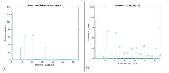
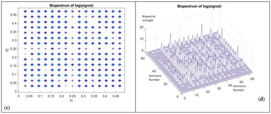
Figure 11.
The two sinusoids and with and going through a quadratic non-linearity gives the spectrum in (a). This composite signal is then fed to a logarithmic non-linearity providing a signal with the specific spectrum in (b). The bispectrum of the signal at the output of the logarithmic non-linearity is presented in two forms (c,d). Both these figures show the extension of the bispectrum to all of the available bispectral region. Bispectral representation is depicted as a carpet which reveals that the bispectral energy covers like a textile the whole bispectral region of interest in points that are additions or subtraction and and their multiples, with strong existence everywhere.
In conclusion:
- The sequential effect of two non-linearities of polynomial type in any order gives an output with bispectrum which normally covers the bispectral region to a certain extent, as defined by the degree of the polynomials.
- In case a logarithmic non-linearity is one of the two sequential non-linearities affecting the signal, then since the output of the logarithmic non-linearity is very rich in bispectral content, the total bispectral content covers all the available bispectral region. This example is depicted graphically in Figure 11a–d.
8. Conclusions
In this work, the effect of specific non-linearities on simple sinusoids was elaborated. In general, new frequencies were created which were phase coupled with the original sinusoids. The way the original frequencies and the new created frequencies were interrelated was extensively investigated. The bispectral space was used to prove the above relationships and to demonstrate graphically the coupled frequencies.
Quadratic, cubic and logarithmic non-linearities were examined as far as their effect on the bispectral signature of their output. Furthermore, simple recommendations were given on how the underlying non-linearity can be detected. The total approach is novel when considering the capability to distinguish from the bispectral content if two non-linearities are simultaneously present.
In the case of a quadratic non-linearity, its output has a restricted number of bispectral peaks even if the original signal contains a dc component. Similarly, in the case of cubic non-linearity, a more extensive coverage of the bispectral region was obtained, although this was again restricted in the area of bispectral region of support. In contrast, the output from the logarithmic non-linearity covered all of the spectral region, although most of the peaks were very weak when they were not close to the origin ().
Finally, when two non-linearities were present in sequential mode then the obtained output had a bispectral content which extended all over the region in which the bispectrum was defined. Accordingly, the presence of two sequential non-linearities can be determined when the bispectral region of support is covered by bispectral peaks.
It was found that the sequential effect of two non-linearities of the polynomial type in any order gives an output with a bispectrum which normally covers the bispectral region to a certain extent, as defined by the degree of the polynomials. In cases when a logarithmic non-linearity is one of the two sequential non-linearities affecting the signal, then since the output of the logarithmic non-linearity is very rich in bispectral content, the total bispectral content covers all of the available bispectral region.
Funding
This research received no external funding.
Data Availability Statement
Data available upon request.
Conflicts of Interest
The author declares no conflict of interest.
References
- Nikias, C.L.; Petropulu, A.P. Higher-Order Spectra Analysis a Nonlinear Signal Processing Framework; Prentice-Hall: Englewood Cliffs, NJ, USA, 1993. [Google Scholar]
- Mendel, J.M. Tutorial on higher-order statistics (spectra) in signal processing and system theory: Theoretical results and some applications. Proc. IEEE 1991, 79, 278–305. [Google Scholar] [CrossRef]
- Peng, Z.K.; Zhang, W.M.; Yang, B.T.; Meng, G.; Chu, F.L. The parametric characteristic of bispectrum for nonlinear systems subjected to Gaussian input. Mech. Syst. Signal. Process. 2013, 36, 456–470. [Google Scholar] [CrossRef]
- Saidi, L.; Ali, J.B.; Fnaiech, F. Bi-spectrum based-EMD applied to the non-stationary vibration signals for bearing faults diagnosis. ISA Trans. 2014, 53, 1650–1660. [Google Scholar] [CrossRef]
- Saidi, L.; Benbouzid, M.; Diallo, D.; Amirat, Y.; Elbouchikhi, E.; Wang, T. Higher-order Spectra Analysis-Based Diagnosis Method of Blades Biofouling in a PMSG Driven Tidal Stream Turbine. Energies 2020, 13, 2888. [Google Scholar] [CrossRef]
- Messina, A.R.; Vittal, V. Assessment of nonlinear interaction between nonlinearly coupled modes using higher order spectra. IEEE Trans. Power Syst. 2005, 20, 375–383. [Google Scholar] [CrossRef]
- Newman, J.; Pidde, A.; Stefanovska, A. Defining the wavelet bispectrum. Appl. Comput. Harmon. Anal. 2021, 51, 171–224. [Google Scholar] [CrossRef]
- Saidi, L.; Fnaiech, F.; Henao, H.; Capolino, G.; Cirrincione, G. Diagnosis of broken-bars fault in induction machines using higher order spectral analysis. ISA Trans. 2013, 52, 140–148. [Google Scholar] [CrossRef]
- Saidi, L. The deterministic bispectrum of coupled harmonic random signals and its application to rotor faults diagnosis considering noise immunity. Appl. Acoust. 2017, 122, 72–87. [Google Scholar] [CrossRef]
- Guo, J.; Shi, Z.; Li, H.; Zhen, D.; Gu, F.; Ball, A.D. Early fault diagnosis for planetary gearbox based wavelet packet energy and modulation signal bispectrum analysis. Sensors 2018, 18, 2908. [Google Scholar] [CrossRef]
- Iglesias-Martínez, M.E.; Antonino-Daviu, J.A.; Fernández de Córdoba, P.; Conejero, J.A. Rotor fault detection in induction motors based on time-frequency analysis using the bispectrum and the autocovariance of stray f lux signals. Energies 2019, 12, 597. [Google Scholar] [CrossRef]
- Zhang, M.; Wang, T.; Tang, T. An imbalance fault detection method based on data normalization and EMD for marine current turbines. ISA Trans. 2017, 68, 302–312. [Google Scholar] [CrossRef]
- Li, Z.; Wang, T.; Wang, Y.; Amirat, Y.; Benbouzid, M.; Diallo, D. A wavelet threshold denoising-based imbalance fault detection method for marine current turbines. IEEE Access 2020, 8, 29815–29825. [Google Scholar] [CrossRef]
- Touimi, K.; Benbouzid, M.E.H.; Tavner, P. Tidal stream turbines: With or without a gearbox? Ocean Eng. 2018, 170, 74–88. [Google Scholar] [CrossRef]
- Titah-Benbouzid, H.; Benbouzid, M.E.H. Biofouling issue on marine renewable energy converters: A state of the art review on impacts and prevention. Int. J. Energy Convers. 2017, 5, 67–78. [Google Scholar] [CrossRef]
- Tian, X.; Gu, J.X.; Rehab, I.; Abdalla, G.M.; Gu, F.; Ball, A. A robust detector for rolling element bearing condition monitoring based on the modulation signal bispectrum and its performance evaluation against the kurtogram. Mech. Syst. Signal. Process. 2018, 100, 167–187. [Google Scholar] [CrossRef]
- Chen, H.; Tang, T.; Ait-Ahmed, N.; Benbouzid, M.E.H.; Machmoum, M.; Zaim, E.H. Attraction, challenge and current status of marine current energy. IEEE Access 2018, 6, 12665–12685. [Google Scholar] [CrossRef]
- Park, H.; Jang, B.; Powers, E.J.; Grady, W.M.; Arapostathis, A. Machine condition monitoring utilizing a novel bispectral change detection. In Proceedings of the 2007 IEEE Power Engineering Society General Meeting, Tampa, FL, USA, 24–28 June 2007; pp. 1–6. [Google Scholar]
- Mitiche, I.; Jenkins, M.D.; Boreham, P.; Nesbitt, A.; Morison, G. An expert system for EMI data classification based on complex Bispectrum representation and deep learning methods. Expert Syst. Appl. 2021, 171, 114568. [Google Scholar] [CrossRef]
- Grover, C.; Turk, N. A novel fault diagnostic system for rolling element bearings using deep transfer learning on bispectrum contour maps. Eng. Sci. Technol. Int. 2022, 31, 101049. [Google Scholar] [CrossRef]
- Xu, Y.; Tang, X.; Sun, X.; Gu, F.; Ball, A.D. A Squeezed Modulation Signal Bispectrum Method for Motor Current Signals Based Gear Fault Diagnosis. IEEE Trans. Instrum. Meas. 2022, 71, 3521508. [Google Scholar] [CrossRef]
- Bollineni, J.; Sharma, A.; Naidu, V. Bispectrum and Convolution Neural Network Based Bearing Fault Diagnosis. In Proceedings of the 4th International Conference on Circuits, Control, Communication and Computing, Bangalore, India, 21–23 December 2022; pp. 456–461. [Google Scholar] [CrossRef]
- Guo, J.; He, Q.; Yang, Y.; Zhen, D.; Gu, F.; Ball, A.D. A local modulation signal bispectrum for multiple amplitude and frequency modulation demodulation in gearbox fault diagnosis. Struct. Health Monit. 2023, 22, 3189–3205. [Google Scholar] [CrossRef]
- Hashempour, Z.; Agahi, H.; Mahmoodzadeh, A. A novel method for fault diagnosis in rolling bearings based on bispectrum signals and combined feature extraction algorithms. Signal Image Video Process. 2022, 16, 1043–1051. [Google Scholar] [CrossRef]
- Cui, L.; Xu, H.; Ge, J.; Cao, M.; Xu, Y.; Xu, W.; Sumarac, D. Use of Bispectrum Analysis to Inspect the Non-Linear Dynamic Characteristics of Beam-Type Structures Containing a Breathing Crack. Sensors 2021, 21, 1177. [Google Scholar] [CrossRef] [PubMed]
- Sharma, A.; Patra, G.K.; Naidu, V.P.S. Bispectral analysis and information fusion technique for bearing fault classification. Meas. Sci. Technol. 2024, 35, 015124. [Google Scholar] [CrossRef]
- Zhu, H.; Li, Q. Target Classification by Conventional Radar Based on Bispectrum and Deep CNN. Prog. Electromagn. Res. C 2023, 130, 127–138. [Google Scholar] [CrossRef]
- Liu, X.; Song, Y.; Chen, K.; Yan, S.; Chen, S.; Shi, B. Modulation Recognition of Low-SNR UAV Radar Signals Based on Bispectral Slices and GA-BP Neural Network. Drones 2023, 7, 472. [Google Scholar] [CrossRef]
- Tassiopoulou, S.; Koukiou, G.; Anastassopoulos, V. Revealing Coupled Periodicities in Sunspot Time Series Using Bispectrum—An Inverse Problem. Appl. Sci. 2024, 14, 1318. [Google Scholar] [CrossRef]
- Huang, L.; Wang, Y.; Liu, J.; Wang, J. Evaluation of ischemic states using bispectrum parameters of EEG and neural networks. In Proceedings of the 26th Annual International Conference of the IEEE Engineering in Medicine and Biology Society, San Francisco, CA, USA, 1–5 September 2004; Volume 1, pp. 582–585. [Google Scholar]
- Schwab, K.; Eiselt, M.; Schelenz, C.; Witte, H. Time-variant parametric estimation of transient quadratic phase couplings during electroencephalographic burst activity. Methods Inf. Med. 2005, 44, 374–383. [Google Scholar] [PubMed]
- Raghavan, R.; Chen, X.; Yip, K.P.; Marsh, D.J.; Chon, K.H. Interactions between TGF-dependent and myogenic oscillations in tubular pressure and whole kidney blood flow in both SDR and SHR. Amer. J. Physiol. Renal. Physiol. 2006, 290, F720–F732. [Google Scholar] [CrossRef]
- Chon, K.H.; Raghavan, R.; Chen, Y.M.; Marsh, D.J.; Yip, K.P. Interactions of TGF-dependent and myogenic oscillations in tubular pressure. Amer. J. Physiol. Renal. Physiol. 2005, 288, F298–F307. [Google Scholar] [CrossRef][Green Version]
- Jamsek, J.; Stefanovska, A.; McClintock, P.V. Nonlinear cardiorespiratory interactions revealed by time-phase bispectral analysis. Phys. Med. Biol. 2004, 49, 4407–4425. [Google Scholar]
- Al-Fahoum, A.; Khadra, L. Combined bispectral and bicoherency approach for catastrophic arrhythmia classification. In Proceedings of the 2005 IEEE Engineering in Medicine and Biology 27th Annual Conference, Shanghai, China, 17–18 January 2006; Volume 1, pp. 332–336. [Google Scholar]
- Wodey, E.; Tirel, O.; Bansard, J.Y.; Terrier, A.; Chanavaz, C.; Harris, R.; Ecoffey, C.; Senhadji, L. Impact of age on both BIS values and EEG bispectrum during anaesthesia with sevoflurane in children. Br. J. Anaesth. 2005, 94, 810–820. [Google Scholar] [CrossRef] [PubMed]
- Bullock, T.H.; Achimowicz, J.Z.; Duckrow, R.B.; Spencer, S.S.; Iragui-Madoz, V.J. Bicoherence of intracranial EEG in sleep, wakefulness and seizures. Electroencephalogr. Clin. Neurophysiol. 1997, 103, 661–678. [Google Scholar] [CrossRef] [PubMed]
- Liu, Z.; Jiang, H.; Zhang, F.; Ouyang, W.; Li, X.; Pan, X. Heart sound classification based on bispectrum features and Vision Transformer mode. Alex. Eng. J. 2023, 85, 49–59. [Google Scholar] [CrossRef]
- Wang, Q.; Jia, X.; Luo, T.; Yu, J.; Xia, S. Deep learning algorithm using bispectrum analysis energy feature maps based on ultrasound radiofrequency signals to detect breast cancer. Front. Oncol. 2023, 13, 272427. [Google Scholar] [CrossRef]
- Li, X.; Zhao, H.; Yu, L.; Chen, H.; Deng, W.; Deng, W. Feature Extraction Using Parameterized Multisynchrosqueezing Transform. IEEE Sens. J. 2022, 22, 14263–14272. [Google Scholar] [CrossRef]
- Hinich, M.J.; Wolinsky, M. Normalizing bispectra. J. Stat. Plan. Inference 2005, 130, 405–411. Available online: https://www.sciencedirect.com/science/article/pii/S0378375804002745?via%3Dihub (accessed on 1 September 2023). [CrossRef]
- Nichols, J.M.; Murphy, K.D. Modeling and detection of delamination in a composite beam: A polyspectral approach. Mech. Syst. Signal. Process. 2010, 24, 365–378. Available online: https://www.sciencedirect.com/science/article/pii/S0888327009002465?via%3Dihub (accessed on 1 September 2023). [CrossRef]
- Nichols, J.; Olson, C.; Michalowicz, J.; Bucholtz, F. The bispectrum and bicoherence for quadratically nonlinear systems subject to non-Gaussian inputs. IEEE Trans. Signal Process. 2009, 57, 3879–3890. Available online: https://ieeexplore.ieee.org/document/5061633 (accessed on 1 September 2023). [CrossRef]
- Wang, X.; Chen, Y.; Ding, M. Testing for statistical significance in bispectra: A surrogate data approach and application to neuroscience. IEEE Trans. Biomed. Eng. 2007, 54, 1974–1982. Available online: https://ieeexplore.ieee.org/document/4352070 (accessed on 1 September 2023).
Disclaimer/Publisher’s Note: The statements, opinions and data contained in all publications are solely those of the individual author(s) and contributor(s) and not of MDPI and/or the editor(s). MDPI and/or the editor(s) disclaim responsibility for any injury to people or property resulting from any ideas, methods, instructions or products referred to in the content. |
© 2024 by the author. Licensee MDPI, Basel, Switzerland. This article is an open access article distributed under the terms and conditions of the Creative Commons Attribution (CC BY) license (https://creativecommons.org/licenses/by/4.0/).