Article

Fusion of Coherent and Non-Coherent Pol-SAR Features for Land Cover Classification

by
Konstantinos Karachristos
,
Georgia Koukiou
and
Vassilis Anastassopoulos
*
Electronics Laboratory, Physics Department, University of Patras, 26504 Rio, Greece
*
Author to whom correspondence should be addressed.
Electronics 2024, 13(3), 634; https://doi.org/10.3390/electronics13030634
Submission received: 4 January 2024 / Revised: 29 January 2024 / Accepted: 31 January 2024 / Published: 2 February 2024

Abstract

:
Remote Sensing plays a fundamental role in acquiring crucial information about the Earth’s surface from a distance, especially through fully polarimetric data, which offers a rich source of information for diverse applications. However, extracting meaningful insights from this intricate data necessitates sophisticated techniques. In addressing this challenge, one predominant trend that has emerged is known as target decomposition techniques. These techniques can be broadly classified into coherent and non-coherent methods. Each of these methods provides high-quality information using different procedures. In this context, this paper introduces innovative feature fusion techniques, amalgamating coherent and non-coherent information. While coherent techniques excel in detailed exploration and specific feature extraction, non-coherent methods offer a broader perspective. Our feature fusion techniques aim to harness the strengths of both approaches, providing a comprehensive and high-quality fusion of information. In the first approach, features derived from Pauli coherent decomposition, Freeman–Durden non-coherent technique, and the Symmetry criterion from Cameron’s stepwise algorithm are combined to construct a sophisticated feature vector. This fusion is achieved using the well-established Fisher Linear Discriminant Analysis algorithm. In the second approach, the Symmetry criterion serves as the basis for fusing coherent and non-coherent coefficients, resulting in the creation of a new feature vector. Both approaches aim to exploit information simultaneously extracted from coherent and non-coherent methods in feature extraction from Remote Sensing data through fusion at the feature level. To evaluate the effectiveness of the feature generated by the proposed fusion techniques, we employ a land cover classification procedure. This involves utilizing a basic classifier, achieving overall accuracies of approximately 82% and 86% for each of the two proposed techniques. Furthermore, the accuracy in individual classes surpasses 92%. The evaluation aims to gauge the effectiveness of the fusion methods in enhancing feature extraction from fully polarimetric data and opens avenues for further exploration in the integration of coherent and non-coherent features for remote sensing applications.

1. Introduction

In the domain of remote sensing data, the techniques of feature and information fusion are employed to combine and integrate diverse sources of information derived from polarimetric features, or different sources [1,2,3]. The goal is to leverage the wealth of information, thereby enhancing the analysis, discrimination, and classification of scenes observed through different sensors. These methodologies contribute to a more thorough understanding of the scattering behavior exhibited by observed targets.
Recent advancements introduced various approaches, primarily grounded in deep learning and machine learning, with the primary objective of intricately integrating polarimetric features. These methodologies are mostly applied to Fully Polarimetric data, among other data types. Notably, inspired by the relationship between model accuracy and feature count, the study [4] employs twelve incoherent target decomposition algorithms and two coherent target decomposition algorithms, resulting in the generation of 79 features. Additionally, 18 polarimetric descriptors and 10 elements of the coherency and covariance matrix are combined to form a feature vector comprising 107 elements for each pixel, serving as the input for subsequent classification. While the classification performance is highly satisfactory, the simultaneous application of all these decomposition techniques appears to pose computational challenges. In [5], Han. F et al. proposed a novel feature fusion method, which is based on the confidence degree according to the Dempster–Shater theory, in order to enhance the robustness and separability of PolSAR extracted features by deep learning models. In the same vein, drawing inspiration primarily from deep learning methodologies, Jiaqiu Ai et al. [6] introduced a PolSAR terrain classification method. This approach involves a sophisticated process that effectively combines low-level texture features with high-level deep features, resulting in notable enhancements in PolSAR terrain classification. In contrast, Yanan Wang et al. [7] opt for a more sophisticated classifier, proposing a convolutional neural network for multichannel fusion based on scattering mechanisms. This network utilizes only three features per PolSAR cell, extracted by the well-established incoherent decomposition technique of Freeman–Durden. The three scattering mechanisms provided by the decomposition algorithm are employed to fuse a new feature output, which in combination with a novel loss function, enhances the classification procedure. Another perspective aiming to integrate polarimetric and spatial features was introduced by Imani Maryam [8]. Specifically, a novel scattering and contextual fusion method based on the complex wavelet transform is introduced, yielding satisfactory results in land cover classification procedures. Likewise, Ref. [9] proposes that the collaborative representation of a PolSAR cell by its neighborhood provides a fused feature space containing both a polarimetric and spatial feature. Furthermore, Ali Sebt M. Darvishnezhad M. [10] introduced a local graph-based fusion method that combines features extracted by Convolutional Neural Networks (CNNs) with their version of Graph Neural Networks (GNNs), referred to as mini GNN.
In another approach [11], rather than relying on features or machine learning algorithms, the focus is on increasing the average peak signal-to-noise ratio (PSNR) and reducing the average mean absolute error (MAE). This is achieved through an image fusion network based on the distinct resolution provided by SAR data. Similarly, Jian et al. [12] present a fusion of data sources incorporating Multispectral and PolSAR images. The objective was to overcome the limitations of poor color information in PolSAR and the low resolution of Multispectral data, aligning with the idea of utilizing diverse data types for comprehensive analysis.
The challenge of employing various sensing methods lies in determining how to integrate information in a meaningful and practical manner. Consequently, ref. [13] introduces a framework for efficiently merging data from optical and polarimetric synthetic aperture radar sensing techniques. The results underscore that combining data from both imaging methods can enhance terrain classification compared to using each modality individually.
The originality of this work is underscored by the novel presentation of two feature fusion techniques, designed to bring a fresh perspective to fully polarimetric data processing for classification procedures. Expanding on this fundamental idea, we intricately combine a non-coherent and a coherent decomposition algorithm, aiming to extract and utilize the information optimally for terrain classification. The first approach employs a fusion procedure utilizing Fisher Linear Discriminant (FLD) analysis, while the second methodology incorporates Cameron’s proposed significant feature of symmetry. This unique combination strives to construct a novel feature vector by seamlessly blending the strengths of coherent and non-coherent algorithms. The deliberate focus on the feature level in our research is a strategic choice to sidestep the complexities associated with combining different types of data. Instead, we capitalize on the distinct ways in which the scattering content of pixels can be interpreted by well-established techniques. This novel approach not only highlights the originality of our contributions but also positions our research as a valuable resource in advancing the field of fully polarimetric data analysis.
The paper is structured as follows: It begins with a concise introduction, initially delving into coherent and non-coherent techniques. Following this, a detailed analysis of the two methods, Pauli and Freeman–Durden decomposition, earmarked for utilization, is provided in Section 3. In Section 4, a thorough examination of the dataset employed in the experimental procedure is conducted. Section 5 unveils the proposed fusion approaches and in Section 6 the evaluation of the proposed features is conducted. Finally, Section 7 encapsulates the drawn conclusions.

2. Coherent and Incoherent Decompositions for Feature Extraction

Polarimetric target decompositions have been introduced to extract features that comprehensively characterize PolSAR (Polarimetric Synthetic Aperture Radar) images. These features serve the purpose of facilitating their utilization in classification and target detection processes. In the existing body of literature, a range of methods and theorems have been proposed for the analysis of the polarimetric scattering matrix, spanning references [14,15,16,17,18,19,20,21,22,23,24,25,26,27,28,29,30,31]. These approaches can be broadly classified into either coherent or non-coherent decomposition techniques [16]. The primary objective of each method is to interpret the information embedded in PolSAR resolution cells, guided by the initial assumption about the nature of the target.

2.1. Coherent Decomposition

In particular, coherent decompositions [14,15,16,17,18,19] operate under the deterministic assumption that each resolution cell contains a singular and dominant scattering mechanism. Consequently, these methodologies strive to extract this dominant scattering behavior and associate it with a fundamental scattering mechanism, typically represented as a simple geometric structure. This extraction process involves expressing the backscattering matrix S , as observed in the HV basis, as a coherent sum of basis matrices. Each basis matrix corresponds to an elementary scattering mechanism, forming the basis for the interpretation and understanding of the complex scattering behavior within PolSAR imagery.

2.2. Non-Coherent Decomposition

On the other hand, non-coherent decomposition techniques [21,22,23,24,25,26,27,28,29,30] have been devised with the premise that the target is spread across multiple adjacent pixels, influenced by the speckle noise inherent in SAR imaging processes. In scenarios where there is no prevalent scattering mechanism within each resolution cell, extracting information necessitates the use of second-order statistics. Non-coherent targets, characterized by their intrinsic stochastic nature, can be discerned by employing the concepts of covariance and coherency matrices. To achieve this, a four-element complex vector is employed, encapsulating the same information as the polarimetric scattering matrix. Subsequently, covariance and coherency matrices are constructed based on this vector, which is defined as follows:
S = S H H S H V S V H S V V k = 1 2 T r a c e S Ψ = [ k 0 , k 1 ,   k 2 ,   k 3 ]
where Ψ is a complete set of 2 × 2 complex basis matrices under the Hermitian inner product [18]. In case of using the lexicographic basis, referred as Borgeaud basis:
Ψ l = 2 1 0 0 0 ,   2 0 1 0 0 ,   2 0 0 1 0 ,   2 0 0 0 1
the corresponding vector is formatted as follows:
k l = S H H ,   S H V ,   S V H ,   S V V T
and the polarimetric covariance matrix C 4 is constructed by the outer product < k l k l > of the scattering vector k l with its conjugate transposed k l :
C 4 v = S H H 2 S H H S H V * S H H S V H * S H H S V V * S H V S H H * S H V 2 S H V S V H * S H V S V V * S V H S H H * S V H S H V * S V H 2 S V H S V V * S V V S H H * S V V S H V * S V V S V H * S V V 2
where   denotes a spatial ensemble averaging assumed homogeneity of the random scattering medium.
Otherwise by using another widely referred basis, the Pauli basis:
Ψ p = 2 1 0 0 1 ,   2 1 0 0 1 , 2 0 1 1 0 , 2 0 i i 0
the vector’s form is:
k p = 1 2 S H H + S V V ,   S H H S V V ,   S H V + S V H ,   i ( S V H S H V ) T
Equivalent to the covariance matrix, the polarimetric coherency matrix is calculated as follows:
T 4 v = < k p k p >
In the absence of ensemble averaging, both matrices depict a deterministic scattering mechanism. These matrices are inherently Hermitian semi-definite matrices, characterized by identical real non-negative eigenvalues. Nevertheless, they diverge in terms of their eigenvectors.

3. Pauli Coherent Decomposition and Freeman–Durden Non-Coherent Approach

3.1. Pauli Decomposition

The fundamental and most well-known coherent decomposition technique is the Pauli approach. The Pauli decomposition serves to express the polarimetric scattering matrix, denoted as S , as a complex sum of the Pauli spin matrices. Each Pauli spin matrix is multiplied by a complex coefficient, signifying an elementary scattering mechanism associated with it:
S = S H H S H V S V H S V V = a 2 S a + b 2 S b + c 2 S c + d 2 S d
where the basis set is defined as:
S a = 1 0 0 1           S b = 1 0 0 1           S c = 0 1 1 0           S d = 0 j j 0
and the Pauli complex coefficients are given by:
a = ( S H H + S V V ) 2   ,   b = ( S H H S V V ) 2 ,   c = ( S H V + S V H ) 2 ,   d = j ( S H V S V H ) 2
These coefficients represent the strength of four superimposed scattering mechanisms, which characterize deterministic targets within each PolSAR cell, and include the following:
  • The single or odd bounce scattering mechanism, denoted as S a , corresponds to plate, sphere, or trihedral scattering;
  • The diplane scattering mechanism, represented by S b , corresponds to dihedral scattering;
  • For a relative orientation of 0°, it denotes even bounce scattering, while for 45°, it corresponds to S c ;
  • The antisymmetric mechanisms are depicted through S d .
Analyzing the amplitudes of these components enables the identification and evaluation of scattering mechanisms within a PolSAR cell.
In the monostatic case, with a single antenna used for both receiving and transmitting (based on the reciprocity theorem for monostatic configuration, S H V = S V H ) , the scattering matrix is expressed as follows:
S = S H H S H V S H V S v v = a S a + b S b + c S c = a 1 0 0 1 + b 1 0 0 1 + c 0 1 1 0
where
a = ( S H H + S V V ) 2   ,   b = ( S H H S V V ) 2 ,   c = 2 S H V
The span of the reduced matrix S can be easily obtained as:
                          S P A N = S H H 2 + S V V 2 + 2 S H V 2 = a 2 + b 2 + c 2
The coefficients’ magnitude can be used to interpret each cell in a PolSAR image. Specifically, the polarimetric data of each cell can be represented by combining the a 2 ,   b 2 ,   c 2 in an RGB image.

3.2. Freeman–Durden Decomposition

As per the classification proposed by J. S. Lee & E. Pottier [15], non-coherent techniques can be categorized into three groups. The first category comprises decompositions grounded in the dichotomy of the Kennaugh matrix [16]. The second category encompasses model-based decompositions [25,26,27,28,29,30], and the third category includes algorithms employing eigenvector analysis [28,29,30].
This study employs the Freeman–Durden three-component decomposition, a foundational and proven technique that has demonstrated success over many years in a diverse range of tasks, owing to its efficacy in handling the distributed nature of targets [32,33,34,35,36]. A brief analysis of the techniques follows.
The Freeman–Durden decomposition method dissects the polarization covariance matrix, dispensing with the necessity for ground truth measurements, and identifies three key components in the radar backscatter phenomenon as follows:
  • Canopy scatter, which arises from a cloud of randomly oriented dipoles or volume;
  • Even- or double-bounce scatter, originating from a pair of orthogonal surfaces with differing dielectric constants;
  • Bragg scatter, emanating from a moderately rough surface.
This integrated scattering model proves invaluable in elucidating the intricacies of polarimetric backscatter from naturally occurring scatterers [22]. The Freeman decomposition shares certain traits with the Pauli-based decomposition, but it offers a more realistic portrayal by incorporating scattering models with dielectric surfaces.
Assuming the absence of any correlation among the volume, even-bounce, and surface scatterer components, the second-order statistics for the collective scattering behavior can be derived by summing the contributions of each distinct scattering mechanism. Consequently, the model for the entire backscatter can be described as:
[ C ] 3 = C 3 v + C 3 d + [ C 3 ] s
where [ C ] 3 is defined as:
[ C ] 3 = S V V 2 2 S V V S V H * S V V S H H * 2 S V H S V V * 2 | S V H | 2 2 S V H S H H * S H H S V V * 2 S H H S V H * S H H 2 =   f v + f d + f s 0 f v 3 + f d α * + f s β * 0 f v 3 0     f v 3 + f d α + f s β 0 f v + f d α 2 + f s β
This model generates four equations involving five unknowns. However, since neither the surface nor the even-bounce scattering mechanism contributes to the HV term, it becomes feasible to directly calculate the volume contribution, which can then be subtracted from the | S H H |   2 , | S V V |   2 , S H H S V V * terms, leaving the three equations below:
S H H 2 = f s β 2 + f d α 2  
S V V 2 = f s + f d  
S H H S V V * = f s β + f d α  
If a particular unknown is held constant, a solution can be ascertained. Van Zyl [24] suggests that the real part of S H H S V V * should be considered to determine whether double bounce scattering, or surface scattering, is prevalent in the residual. If R e S h h S v v * 0 , surface scattering is regarded as dominant, and the parameter α is fixed at α = 1 . If R e S h h S v v * is negative, double bounce scattering is deemed dominant, and the parameter β is fixed at β = 1 . The estimations for the contributions of f s and f d , along with parameters α and β, can be derived from the residual radar measurements. Ultimately, the contribution of each scattering mechanism to the span can be assessed:
S p a n = S H H 2 + 2 S H V 2 + S V V 2 = P s + P d + P v
where
P s = f s 1 + β 2
P d = f d 1 + a 2
P v = 8 3 f v

3.3. Cameron’s Angle of Symmetry
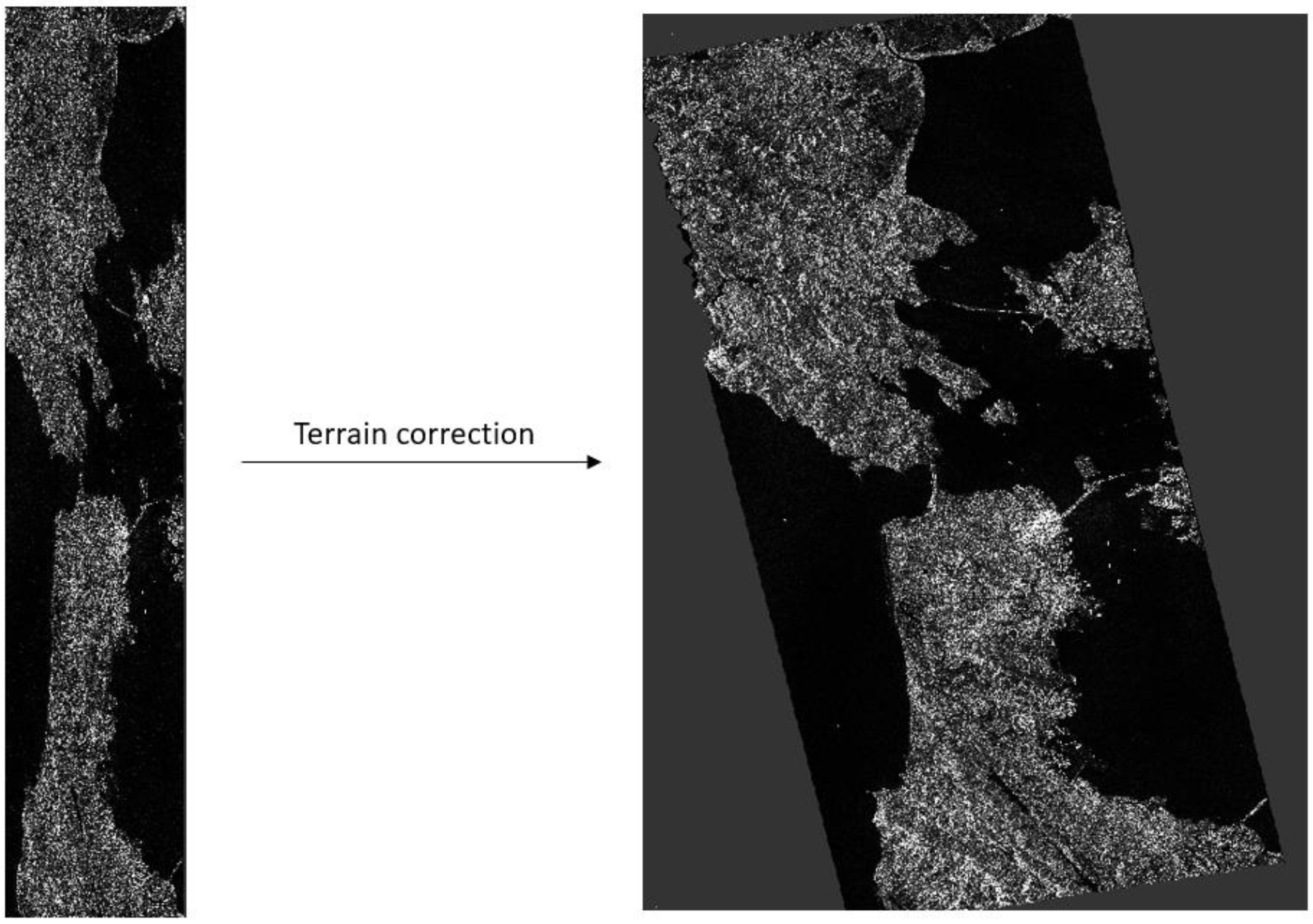
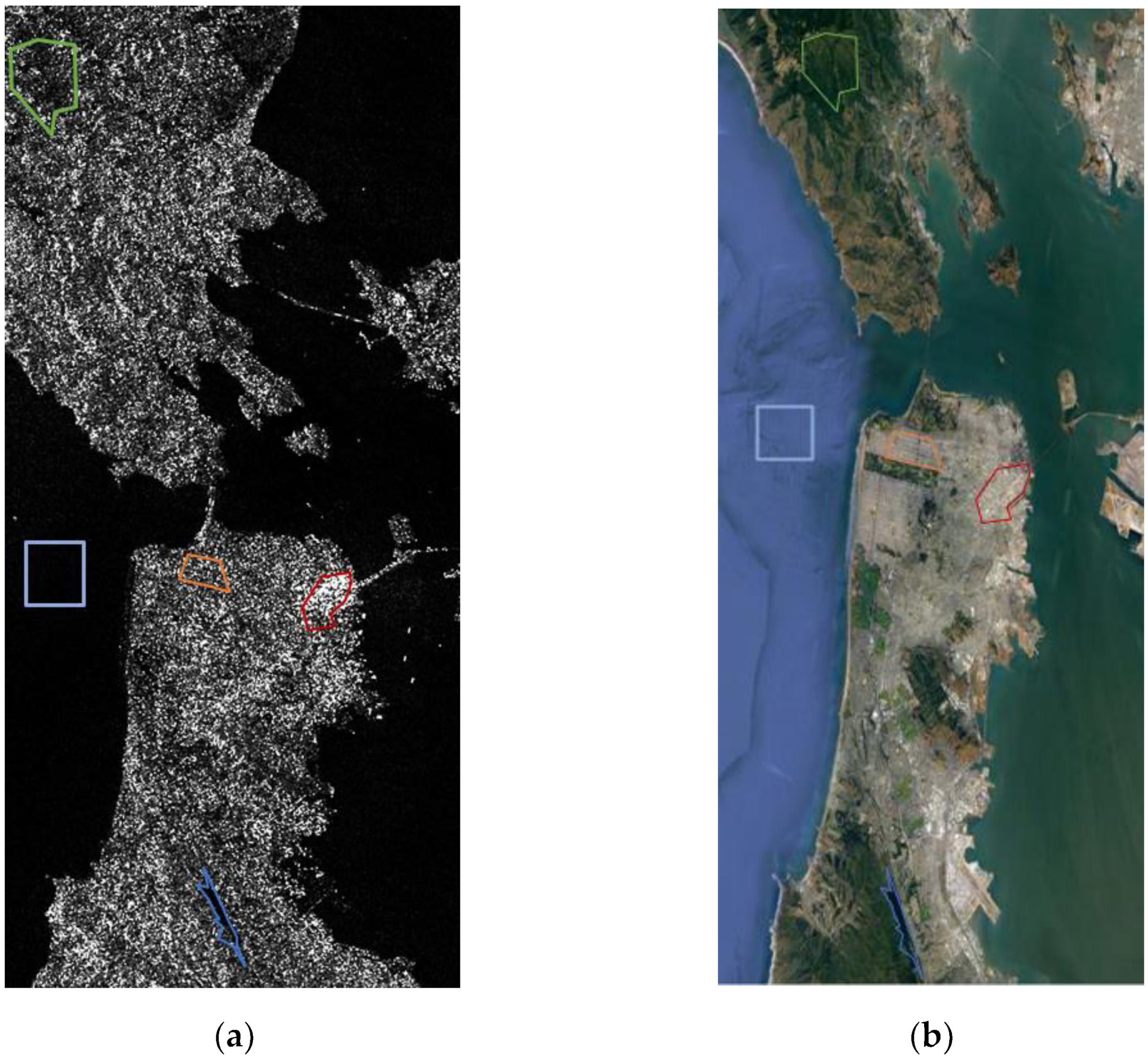
Cameron’s decomposition builds upon Pauli’s methodology, introducing a notable innovation by incorporating the concept of symmetry. The decomposition process consists of two stages: Initially, the scattering matrix undergoes decomposition into its reciprocal and non-reciprocal components through the application of the angle θ r e c . Subsequently, the reciprocal term undergoes a secondary decomposition into its symmetric and non-symmetric components, facilitated by the angle τ s y m .
Cameron’s Coherent Target Decomposition (CTD) analysis [18,19,20] integrates Huynen’s hypothesis [21] regarding the two fundamental properties of scatterers: reciprocity and symmetry. A scatterer is deemed reciprocal when its backscattering matrix’s non-diagonal elements are pairwise equal. Reciprocity holds true for all monostatic Synthetic Aperture Radar (SAR) systems, given that transmitting and receiving antennas are co-located. Consequently, all scatterers imaged by monostatic SAR systems are considered reciprocal. A reciprocal scatterer is further classified as symmetric if it exhibits an axis of symmetry in the plane perpendicular to the radar line of sight (LOS).
Transforming the scattering matrix S into a vectorial form, for computational simplicity and efficiency, yields the following expression based on Pauli decomposition:
s = V S = α s ^ a + β s ^ b + γ s ^ c + δ s ^ d
The hat s ^ of vector s symbolizes a unit vector ( s ^ = 1 , where | | stands for vector magnitude).
Based on the reciprocity theorem, according to which S H V = S V H , Cameron divides the respective target into either reciprocal or non-reciprocal, by the projection angle θ r e c in the reciprocal subspace, as follows:
θ r e c = cos 1 P r e c S , 0 θ r e c π 2
where
P r e c = 1 0 0 0 0 1 2 1 2 0 0 1 2 1 2 0 0 0 0 1
If θ r e c 45 o the elementary scattering mechanism is considered as reciprocal, otherwise it is taken as non-reciprocal. The scattering matrix of a reciprocal scatterer is now decomposed as:
S = S r e c = α s ^ a + β s ^ b + γ s ^ c
where
α = S H H + S V V 2 , β = S H H S V V 2 , γ = 2 S H V
Ultimately, the reciprocal scatterer is expressed as follows:
s r e c = α 1 2 1 0 0 1 + β 1 2 1 0 0 1 + γ 1 2 0 1 1 0
The symmetric classification of a reciprocal scatterer is established when the target exhibits an axis of symmetry in the plane perpendicular to the radar Line of Sight (LOS). Alternatively, symmetry is affirmed if a rotation angle ψ c exists, nullifying the projection of S r e c on the antisymmetric component S c . The presence of such an angle ensures that the symmetric component of the reciprocal scatterer attains its maximum value. This rotation angle, ψ c , corresponds to the orientation angle of the scatterer. The peak value of the symmetric component of the reciprocal scatterer is defined as follows:
S s y m m a x = α S a + ε S b
with
ε = β c o s χ + γ s i n χ
and
t a n 2 χ = β γ * + β * γ ( β 2 + γ 2 )
when β  γ . Alternatively, if β  = γ then χ = 0 . The orientation angle of the scatterer can be found as follows:
ψ = 1 4 χ ,           π χ π
As for the degree of symmetry, it is expressed as the degree to which S deviates from S s y m m a x and it can be calculated as:
cos   τ sym = | ( S ,   S sym max ) | S S sym max | | , 0 τ s y m π 4
where | | | | stands for the norm of a complex vector form to which the matrix corresponds.
If τ s y m = 0 then the scattering matrix corresponds to a perfectly symmetric target. If τ s y m = π 4 the target that backscattered the radiation is considered asymmetric. Cameron considers as symmetric any elementary scatterer with angle τ s y m π 8 , otherwise he considers it as asymmetric.

4. Dataset

The evaluation of the proposed fusion approach involving both coherent and non-coherent algorithms was conducted using the benchmark fully polarimetric dataset of San Francisco Bay. Specifically, the Level-1 Single Look Complex (SLC) product from RADARSAT-2 was employed for this purpose. RADARSAT-2, a satellite system developed by the Canadian Space Agency, operates in the C-band. The acquired images utilized the Fine Quad-Pol Beam mode, providing full polarimetric imaging with a nominal resolution of 5.2 × 7.6 [Range × Azimuth] (m) and swath widths of approximately 25 km. This coverage spans from an incidence angle of 18 degrees to at least 49 degrees.
SLC images are characterized by complex (I and Q) magnitude values, encompassing both amplitude and phase information. Radiometric calibration processes were essential for handling SLC data, converting raw digital image data from the satellite to a standardized physical scale based on known reflectance measurements from ground surface objects. The calibration procedure took place within the Sentinel Application Platform (SNAP) environment, a universal architecture for various Sentinel Toolboxes, and was provided free of charge by ESA/ESRIN to the Earth Observation Community [37].
The image, initially in the acquisition geometry of the sensor, introduced distortions associated with the side-looking geometry. To address this, geocoding was imperative. This was achieved through the application of the range Doppler orthorectification method within the SNAP platform, in conjunction with the calibration process. The range Doppler terrain correction operator utilized orbit state vector information, radar timing annotations, slant to ground range conversion parameters, and reference digital elevation model data to derive precise geolocation information. The data transformation process is illustrated in Figure 1.
For the selection of different land cover types, we relied on the alignment between the geocoded image and the corresponding region on Google Earth, as depicted below (Figure 2).

5. Fusing Coherent and Non-Coherent SAR Features

5.1. Fusion Approaches for Comprehensive Information Integration

The objective of the current study is to propose two refined approaches for fusing features extracted from the aforementioned techniques. These methods are designed to effectively consolidate a substantial amount of information from both coherent techniques and incoherent ones into a unified feature vector.
To accomplish this objective, the initial approach leverages seven features extracted through the coherent Pauli decomposition and Freeman–Durden non-coherent methodology. Additionally, it explores the angle of symmetry as initially proposed in Cameron target decomposition. These features collectively form a seven-component vector that serves as an input for the well-established FLD analysis scheme. Consequently, a set of new features is derived through a linear combination of these vectors. This novel feature set is then presented as a result of the analytical process. Rather than consolidating features into a new vector and introducing a novel feature space, the second proposed methodology investigates how information is distributed, whether it is concentrated within a single pixel or spatially dispersed in a neighborhood. This exploration is achieved by analyzing the symmetrical degree of the scattering matrix that describes the target under examination. The angle of symmetry is employed as the criterion for constructing a unique feature vector, achieved through the fusion of coefficients from both Pauli and Freeman–Durden techniques.

5.2. Feature Fusion Utilizing FLD

In this subsection we elaborate on the statistics of the features for each separate class as well as the distribution and the separability of the classes in the 7D feature space.
The covariance of each class indicates the degree of the extent of the features towards various directions as well as their correlation. The correlation of the features in each class is clearly indicated by the correlation coefficient matrix. However, the extent of the features of each class in the feature space is mainly provided by the eigenvalues of the covariance matrix. It is very well known that each semi-axis (on a specific eigenvector) of the 7D hyper ellipsoid, which represents a specific class, is analogous to the square root of the corresponding eigenvalue.
In the following the correlation coefficient matrix, the eigenvalues and their squared root are provided for the class of the city.
From Table 1. It is evident that there exists a strong correlation between many of the features for the city class especially for the couples where the correlation coefficient is of the order of 0.1 or larger. Furthermore, the eigenvalues of the 7D cluster which correspond to the city region along with their squared roots are provided in Table 2. Accordingly, it is evident that all axes of the 7D hyper ellipsoid are of significant extent, with the largest being 3 times longer than the shorter one. The same happens for the rest of the clusters of our experiment (Table 3).

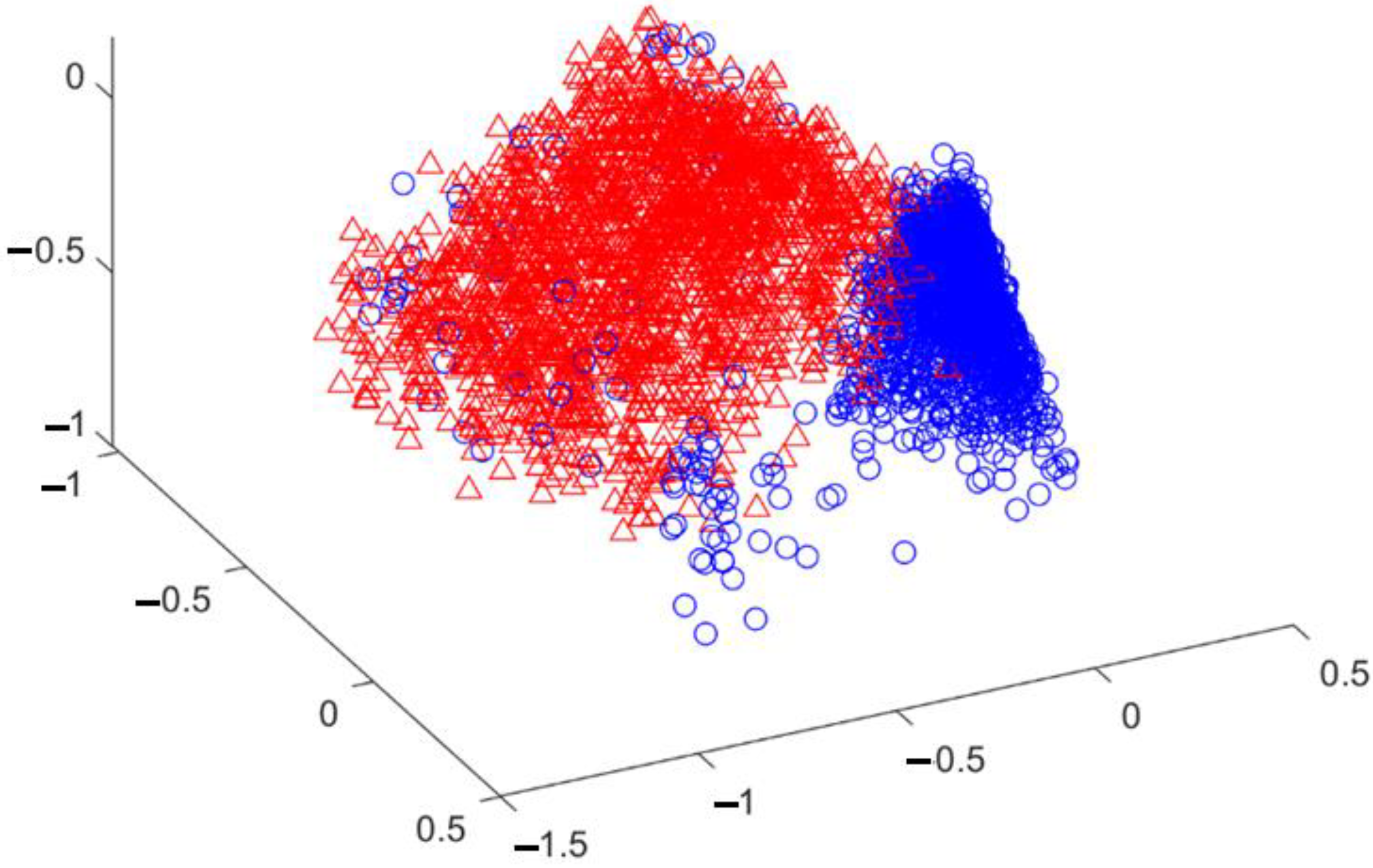
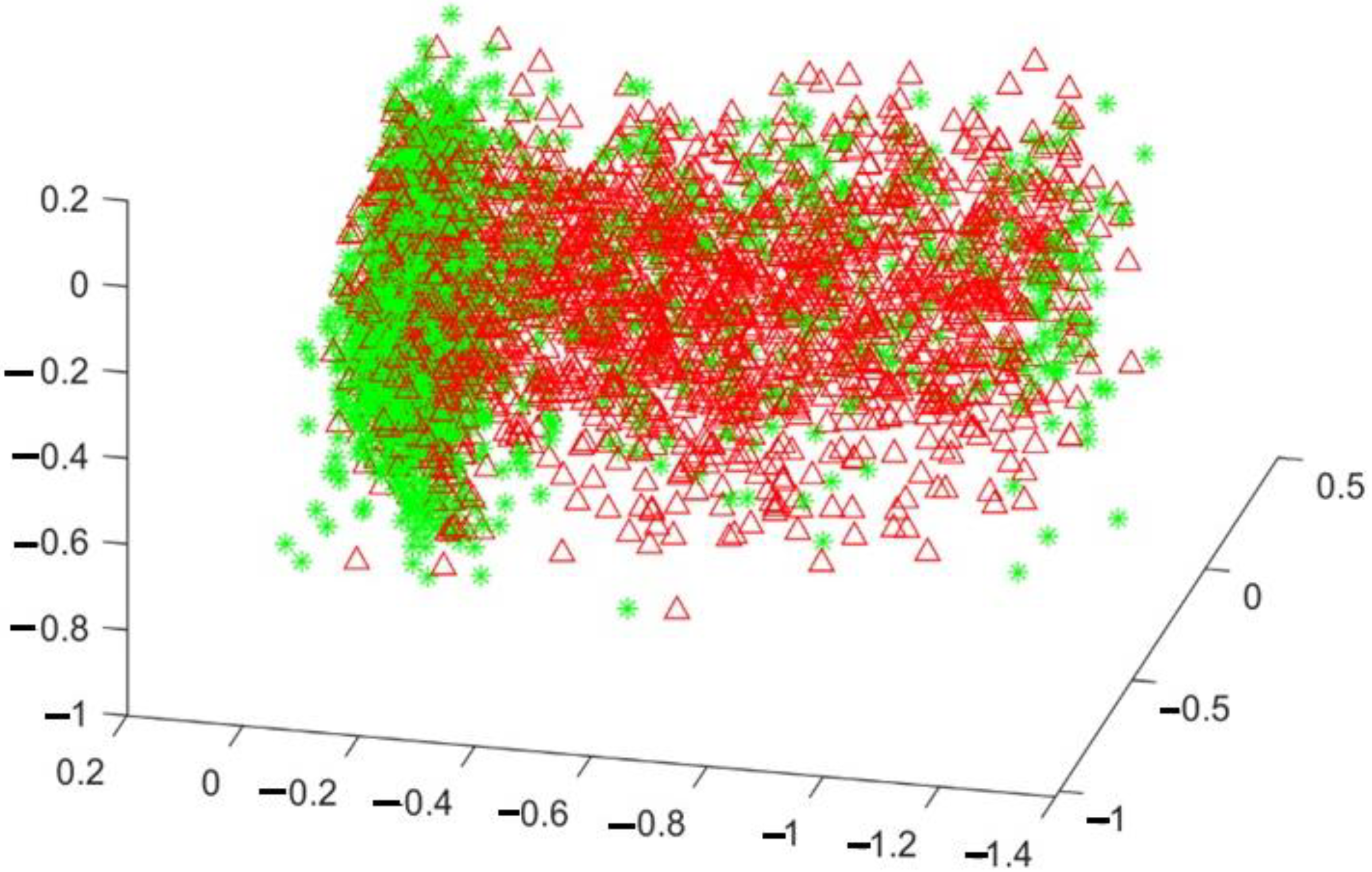
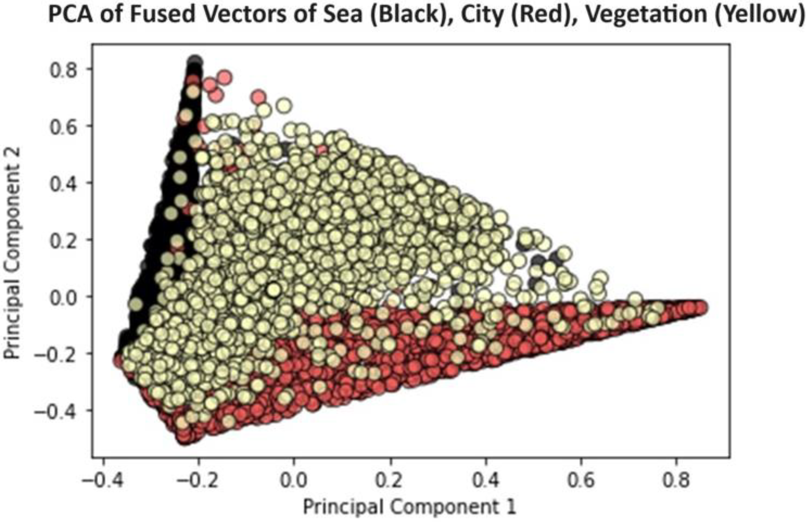
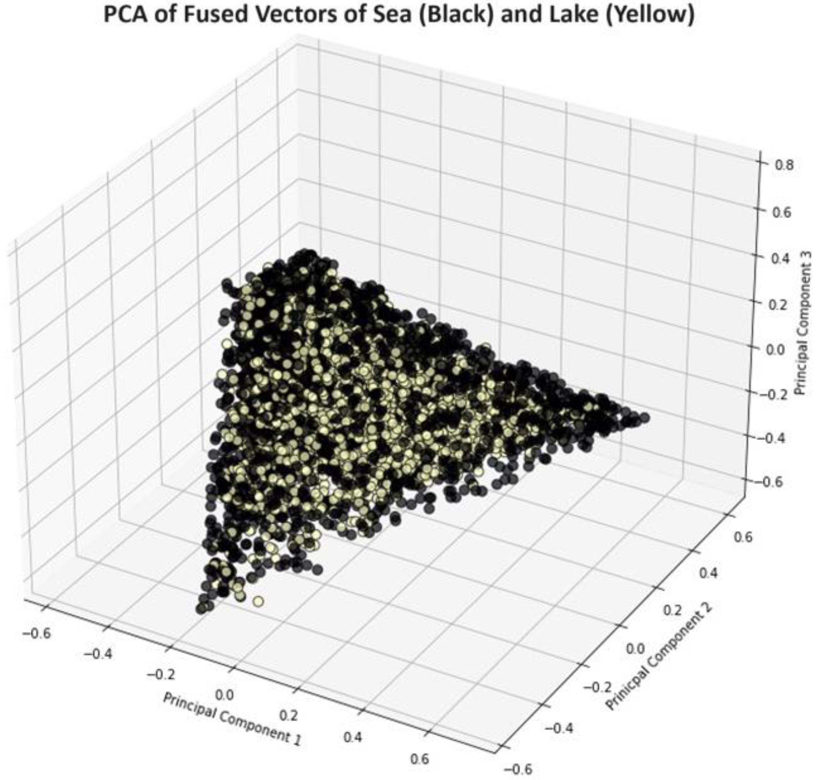
5.3. Dimensionality Reduction–Direction of Fused Features

Dimensionality reduction from 7 dimensions onto three dimensions is necessary to perceptually understand the separability of the clusters. It is achieved by means of the FLD method [38], i.e., the projection by means of a suitable linear transformation W in a new space. The vectors wi of W are the new directions where each 7D vector vi, derived as explained in the previous sections, will be projected. This linear transformation is:
y i = W t v i
where yi is the transformed vi. One of the important criteria used for best separating the clusters is given by maximizing the function J(w) in the transformed space [38]:
J w = w t S B w w t S W w
The transformation vectors w i of W are obtained from the solution of the generalized eigenvalue problem:
S B w i = λ i S W w i
where SW is called the within-scatter-matrix while SB is the between-scatter-matrix. The solution of Equation (36) gives the eigenvalues which correspond to each of the above eigenvectors w i . From this solution we will employ the most important directions corresponding to the largest eigenvalues. Accordingly, the sum of the three largest eigenvalues over the sum of all eigenvalues gives the quality of cluster separability in the reduced 3D feature space. The largest eigenvalues obtained are those given in Table 4.
It is well known that the separability information in each direction is relevant to the square root of the corresponding eigenvalues. Accordingly, almost 90% of the information for cluster separability is held in the three directions corresponding to the first three largest eigenvalues. Obviously, the clusters are separable even though we are working in the three dimensions which correspond to the three largest eigenvalues. We have to mention that since we have a 5-class problem only 4 eigenvalues are non-zero, while the use of the rest dimensions can support better separability. For demonstration purposes, two pairs of clusters in our experiment are demonstrated (Figure 3 and Figure 4) in the 3D space determined by the eigenvectors corresponding to the largest eigenvalues.
In practice, using neural networks with all available inputs, the separability information distributed in all feature space dimensions is taken into consideration. This gives the neural structures the superiority of giving higher class separability.

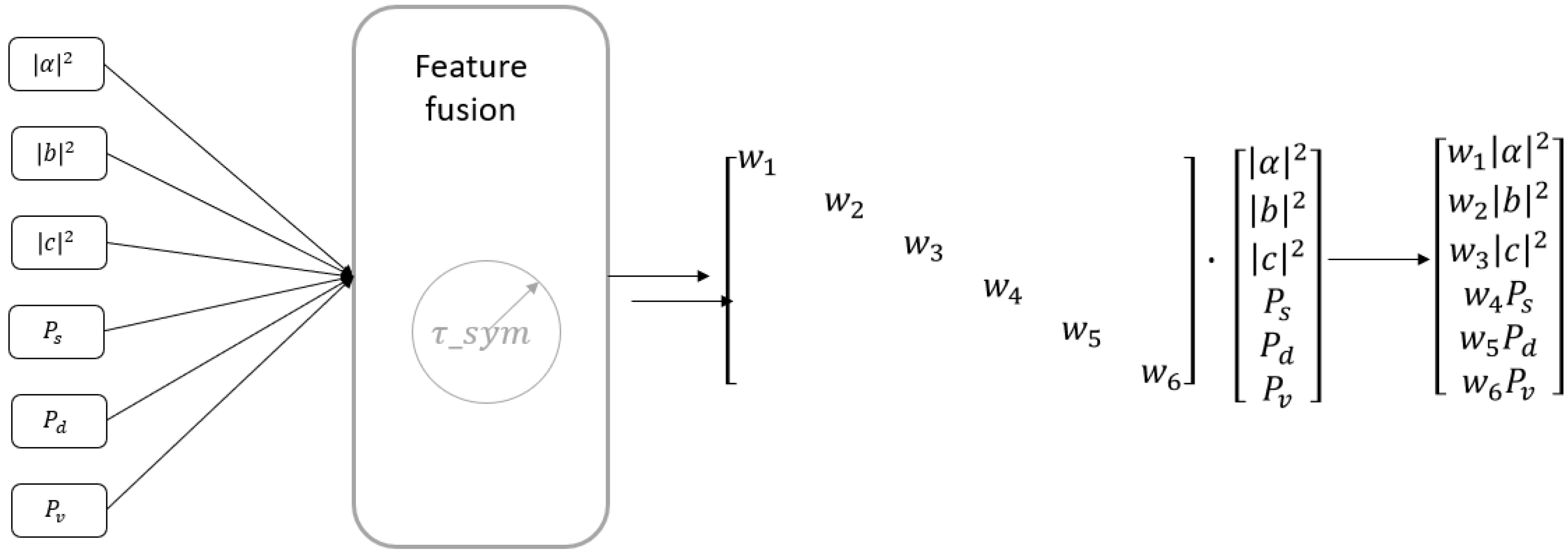
5.4. Feature Fusion Using the Angle of Symmetry

Regarding the methodology that incorporates the angle of symmetry proposed by Cameron as a criterion for constructing a new vector, rather than merely a component of a new feature, the central tenet is in the manner in which a target is deemed symmetric according to Cameron’s methodology. Specifically, adhering to Cameron’s algorithm, if the scattering matrix corresponding to a target under examination is reciprocal, the subsequent step involves assessing symmetry through the angle introduced in Equation (33).
Cameron posited that a target can be classified as symmetrical if this angle falls within the interval of 0–45 degrees, has a value lower than the half, specifically below 22.5 degrees. Extending this conceptual framework and integrating it with the fundamental disparity between coherent and non-coherent approaches—predicated on the distribution of the target across neighboring pixels in non-coherent methods, as opposed to its confinement within a single cell in coherent methods—the principal aspect of this approach emerges.
If the angle of symmetry is less than 11.25 degrees, constituting the half threshold of Cameron’s proposal, we can infer that almost all of the relevant information is encompassed within the specific cell under examination, with only minimal information disseminated into the pixel’s vicinity. Conversely, if this angle exceeds 11.25 degrees, the information pertaining to the target appears to be distributed across multiple pixels, aligning with the non-coherent approach.
To formalize this conceptual framework into an algorithm, we employ the angle of symmetry as a criterion, partitioning weights into six coefficients: 3 corresponding to the Pauli coherent decomposition and 3 to the Freeman–Durden non-coherent technique. Consequently, when the target exhibits high symmetry, the weights corresponding to the coherent approach assume greater significance compared to those associated with the non-coherent approach. Conversely, as the angle of symmetry surpasses 11.25 degrees, the weights of the coefficients aligned with the non-coherent technique become more prominent. When the angle of symmetry deviates from the prescribed symmetry boundaries, the cell corresponds to an asymmetric case. To achieve this, the concept of symmetry angle introduced by Cameron [13] is employed to establish the significance weights among all features. The outlined approach can be succinctly summarized in the following workflow (Figure 5):
In an effort to visualize the feature vectors crafted through this approach, we employ Principal Component Analysis (PCA). This technique is utilized to extract the two most significant components, capturing the utmost informational content. The objective is to generate 2D representations that vividly illustrate the feature vectors associated with each distinct land cover (Figure 6 and Figure 7). Additionally, as previously implemented, the same neural network is employed to conduct a comprehensive classification procedure. This serves to underscore the efficacy and quality of these newly fused features.
As has already been studied, differentiating between the lake and the sea proves to be the most challenging aspect. Therefore, in this specific case, the three components of PCA are employed to illustrate how these features are positioned within the feature space.
The evaluation of the second feature vector, produced through this fusion procedure, is scrutinized using the same neural network employed in the first feature fusion approach to facilitate a more comprehensive comparison.

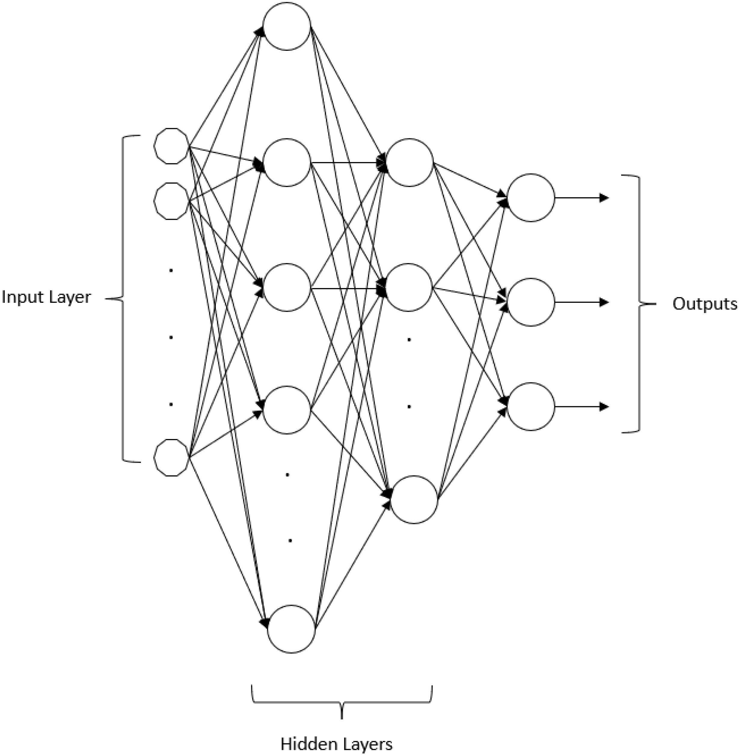
6. Evaluation of the Fused Features in a Land Cover Classification Procedure Based on a Simple Neural Network

As previously mentioned, to assess the robustness and significance of the feature vectors generated through the two proposed fusion techniques, a land cover classification procedure is employed. The evaluation utilizes a well-established neural network classifier with a deliberately simple architecture. This choice ensures that accuracy primarily relies on the sophisticated nature of the features and the information they encapsulate, rather than being overly influenced by the elegance of the classifier.
In its broadest sense, a neural network is a computational model designed to emulate the cognitive processes of the human brain in addressing specific tasks or functions. To attain optimal performance, neural networks deploy an extensive network of basic computing units known as “neurons” or processing units. The network acquires knowledge from its environment through a learning process. Synaptic weights, representing interneuron connection strengths, are employed to store acquired knowledge. The learning process is executed through a learning algorithm, tasked with systematically modifying the synaptic weights of the network to achieve a predetermined design objective. The Multilayer Perceptron (MLP) neural network, a model employing single or multi-layer perceptrons to approximate input–output relationships, stands out as the most widely used network model for image classification in remote sensing [39,40]. Typically, the network comprises sensory units forming the input layer, one or more hidden layers of computational units, and an output layer (Figure 8). The essential components of the MLP include the network’s architecture, consisting of a number of neurons and layers, and the learning algorithm. Supervised backpropagation (BP) is the prevalent training algorithm for MLP networks [41], grounded in the error-correction learning rule. The error backpropagation learning process involves two passes through the network layers: a forward pass and a backward pass. During the forward pass, an input vector is applied to the sensory nodes, and its impact propagates through the network layers, culminating in the generation of outputs. Synaptic weights remain fixed during the forward pass. In the backward pass, synaptic weights are adjusted based on an error-correction rule. Specifically, the actual network response is subtracted from the desired response, generating an error signal that propagates backward through the network, hence the term “error backpropagation”. Synaptic weights are then adjusted to align the actual response statistically closer to the desired response. Beyond the MLP architecture and learning algorithm, operational factors such as data characteristics and training parameters can influence model performance. However, these considerations are application specific and will be addressed in conjunction with the case study in the subsequent section.
The neural network designed for this research is a fully interconnected linkage of three layers. The input layer is composed of 7 neurons in the first experimental procedure, in which the feature fused based on FLD analysis is examined, and 6 of which are in the second fusion case. Two layers including 18 and 12 neurons, respectively, are termed the hidden layers. The output layer is composed of 4 neurons representing the target classes of land covers (sea, city, vegetation, and suburban) that were to be produced by the network. Every neuron within one layer is fully interconnected with the neurons in the adjacent layers. The activation function in the present task is the sigmoid function:
f x = 1 1 + e x
The sigmoid function’s monotonic, continuous, and differentiable nature, combined with its derivative expressible in terms of itself, simplifies the derivation of update equations for weight learning in a neural network using the backpropagation algorithm, as employed in our developed network. Typically, the backpropagation algorithm utilizes a gradient-based approach for learning neural network weights. In our case, the “adam” optimizer was chosen, and a comprehensive description of this optimization method can be found in the work by Diederik P. Kingma and Jimmy Lei Ba [42].
In the designed MLP network, epoch training is preferred for its efficiency and stability over pixel-by-pixel training [43]. An epoch involves passing the entire dataset forward and backward through the neural network once. Given the impracticality of processing the entire epoch at once, it is divided into smaller batches. The batch size, a key hyperparameter in the proposed ANN, denotes the total number of training samples passed through the network at once. For this study, 5000 epochs were selected to acquire ample knowledge of class membership from the training dataset, ensuring avoidance of overtraining, while the batch size is set to 128 to promote effective generalization on the data.
To assess the model’s performance on the available dataset, k-fold cross-validation was implemented. The dataset is partitioned into K folds, with each fold used to evaluate the model’s performance when exposed to new data. In our study, K is set to 5, constituting a 5-fold cross-validation. Each fold serves as a testing set at one point in the process.
The outcomes are consolidated in Table 5, accompanied by a more detailed interpretation elucidated through the examination of confusion matrices in Figure 9a,b. The evaluation of classification accuracy is a crucial aspect in validating the effectiveness of proposed techniques within a scientific paper. In our study, we meticulously examined the accuracy percentages across various folds, affirming the reliability of the introduced feature fusion methodologies and emphasizing the prevention of overfitting in our classification system.
Our approach involved utilizing a feature fusion technique, where the symmetry angle served as a criterion for weight distribution. Notably, we observed a slightly elevated success rate, reaching an average of 86%. Furthermore, even when fusing features based on Fisher’s Linear Discriminant (FLD) analysis, our results remained satisfactory, exhibiting success rates ranging from 81% to 83% across different folds. It is essential to acknowledge that these results are preliminary, and the potential for optimization, from data selection to classification processes, could further enhance the accuracy of our proposed techniques. This optimism underscores our belief in the promising nature of these feature fusion approaches.
A detailed examination of the confusion matrices provides deeper insights into our findings. Notably, within the sea category, characterized by homogeneity, our classification success rates surpassed 92% in both scenarios. However, challenges emerged in distinguishing vegetation land cover, with the lowest percentages recorded. Specifically, using the first feature fusion method, only 61% of samples were successfully classified as vegetation, with the remainder erroneously categorized as part of the urban fabric. This misclassification can be attributed to less rigorous region selection, allowing the inclusion of vegetation patches in urban fabric and vice versa. Additionally, preprocessing procedures played a pivotal role, as both urban and vegetation targets appeared dispersed across multiple PolSAR cells, contributing to lower accuracy percentages.
Applying the second feature fusion methodology yielded remarkable success rates of 96% in classifying PolSAR cells within urban areas. While this method displayed notable proficiency, confusion was observed primarily between suburban and vegetation categories, as anticipated. Nonetheless, the overall process demonstrated high satisfaction. It is important to note that addressing dark spots through more precise area selection and sophisticated preprocessing is an avenue for potential improvement, albeit beyond the scope of this current work.
In summary, our comprehensive analysis of classification accuracy, bolstered by detailed examination through confusion matrices, underscores the robustness of our proposed techniques. The identified challenges provide valuable insights for future refinement, emphasizing the ongoing evolution and optimization of our methodologies.

7. Conclusions

Our research endeavors to showcase the innovation stemming from advanced fusion processes utilizing fully polarimetric data. By integrating both coherent and non-coherent techniques at the feature level, our synthesized algorithms exhibit promise for the fusion of satellite data during feature extraction. This unique approach combines the precision of coherent techniques, especially beneficial in PolSAR cell-targeted scenarios, with the ability to provide detailed target descriptions when scattering behavior extends across PolSAR cell neighborhoods. The validation of our fusion procedures through land cover classification, employing a straightforward neural network, underscores our primary focus on emphasizing the quality and robustness of the introduced fused feature vectors. Despite the simplicity of our classification approach, we achieve notable accuracy rates. Graphical representations further illustrate the clear separation of vectors in the feature space, even in areas prone to entanglement, such as those representing lakes and seas.
This research establishes that the concurrent application and fusion of coherent and non-coherent techniques, particularly at the feature level, holds significant promise in elevating accuracy in computer vision and machine learning processes. The fused features not only contribute to constructing sophisticated classifiers but also showcase impressive speed and accuracy. Derived from just three decomposition techniques applied to satellite data, our findings advocate for a comprehensive exploration of feature fusion techniques within the realm of remote sensing information extraction. The potential demonstrated herein paves the way for further advancements in the optimization of performance and accuracy in this critical field.

Author Contributions

K.K., G.K. and V.A. have equally contributed to Conceptualization, Methodology, Validation, and Writing—Original Draft Preparation. All authors have read and agreed to the published version of the manuscript.

Funding

No funding was received for conducting this study.

Data Availability Statement

Data availability for reasonable requests.

Conflicts of Interest

The authors declare no conflict of interest.

References

  1. Simone, G.; Farina, A.; Morabito, F.C.; Serpico, S.B.; Bruzzone, L. Image fusion techniques for remote sensing applications. Inf. Fusion 2002, 3, 3–15. [Google Scholar] [CrossRef]
  2. Gómez-Chova, L.; Tuia, D.; Moser, G.; Camps-Valls, G. Multimodal Classification of Remote Sensing Images: A Review and Future Directions. Proc. IEEE 2015, 103, 1560–1584. [Google Scholar] [CrossRef]
  3. Alparone, L.; Bruno Aiazzi, B.; Baronti, S.; Garzelli, A. Remote Sensing Image Fusion, 1st ed.; Routledge Taylor & Francis Group: London, UK, 2015. [Google Scholar]
  4. Ni, J.; Zhang, F.; Yin, Q.; Li, H.C. Robust weighting nearest regularized subspace classifier for PolSAR imagery. IEEE Signal Process. Lett. 2019, 26, 1496–1500. [Google Scholar] [CrossRef]
  5. Han, F.; Zhang, L.; Dong, H. Trusted Polarimetric Feature Fusion for Polsar Image Classification. In Proceedings of the 2023 SAR in Big Data Era (BIGSARDATA), Beijing, China, 20–22 September 2023; pp. 1–4. [Google Scholar] [CrossRef]
  6. Ai, J.; Wang, F.; Mao, Y.; Luo, Q.; Yao, B.; Yan, H.; Xing, M.; Wu, Y. A Fine PolSAR Terrain Classification Algorithm Using the Texture Feature Fusion-Based Improved Convolutional Autoencoder. IEEE Trans. Geosci. Remote Sens. 2022, 60, 5218714. [Google Scholar] [CrossRef]
  7. Wang, Y.; Cheng, J.; Zhou, Y.; Zhang, F.; Yin, Q. A Multichannel Fusion Convolutional Neural Network Based on Scattering Mechanism for PolSAR Image Classification. IEEE Geosci. Remote Sens. Lett. 2022, 19, 4007805. [Google Scholar] [CrossRef]
  8. Imani, M. Scattering and contextual features fusion using a complex multi-scale decomposition for polarimetric SAR image classification. Geocarto Int. 2022, 37, 17216–17241. [Google Scholar] [CrossRef]
  9. Imani, M. Scattering and Regional Features Fusion Using Collaborative Representation for PolSAR Image Classification. In Proceedings of the 2022 9th Iranian Joint Congress on Fuzzy and Intelligent Systems (CFIS), Bam, Iran, 2–4 March 2022; pp. 1–6. [Google Scholar] [CrossRef]
  10. Sebt, M.A.; Darvishnezhad, M. Feature fusion method based on local binary graph for PolSAR image classification. IET Radar Sonar Navig. 2023, 17, 939954. [Google Scholar] [CrossRef]
  11. Lin, L.; Li, J.; Shen, H.; Zhao, L.; Yuan, Q.; Li, X. Low-Resolution Fully Polarimetric SAR and High-Resolution Single-Polarization SAR Image Fusion Network. IEEE Trans. Geosci. Remote Sens. 2022, 60, 5216117. [Google Scholar] [CrossRef]
  12. Wang, J.; Chen, J.; Wang, Q. Fusion of POLSAR and Multispectral Satellite Images: A New Insight for Image Fusion. In Proceedings of the 2020 IEEE International Conference on Computational Electromagnetics (ICCEM), Singapore, 24–26 August 2020; pp. 83–84. [Google Scholar] [CrossRef]
  13. West, R.D.; Yocky, D.A.; Redman, B.J.; Van Der Laan, J.D.; Anderson, D.Z. Optical and Polarimetric SAR Data Fusion Terrain Classification Using Probabilistic Feature Fusion. In Proceedings of the 2020 IEEE International Geoscience and Remote Sensing Symposium, Waikoloa, HI, USA, 26 September–2 October 2020; pp. 2097–2100. [Google Scholar] [CrossRef]
  14. Touzi, R.; Boerner, W.M.; Lee, J.S.; Lueneburg, E. A review of polarimetry in the context of synthetic aperture radar: Concepts and information extraction. Can. J. Remote Sens. 2004, 30, 380–407. [Google Scholar] [CrossRef]
  15. Lee, J.S.; Pottier, E. Polarimetric Radar Imaging, 1st ed.; CRC Press: New York, NY, USA, 2009. [Google Scholar]
  16. López-Martínez, C.; Pottier, E. Basic Principles of SAR Polarimetry. In Polarimetric Synthetic Aperture Radar, 1st ed.; Hajnsek, I., Desnos, Y.L., Eds.; Springer: Cham, Switzerland, 2021; Volume 25, pp. 1–58. [Google Scholar] [CrossRef]
  17. Krogager, E. New decomposition of the radar target scattering matrix. Electron. Lett. 1990, 26, 1525–1527. [Google Scholar] [CrossRef]
  18. Cameron, W.L.; Leung, L.K. Feature Motivated Polarization Scattering Matrix Decomposition. In Proceedings of the IEEE International Conference on Radar, Arlington, VA, USA, 7–10 May 1990. [Google Scholar]
  19. Cameron, W.L.; Youssef, N.N.; Leung, L.K. Simulated Polarimetric Signatures of Primitive Geometrical Shapes. IEEE Trans. Geosci. Remote Sens. 1996, 34, 793–803. [Google Scholar] [CrossRef]
  20. Cameron, W.L.; Rais, H. Conservative Polarimetric Scatterers and Their Role in Incorrect Extensions of the Cameron Decomposition. IEEE Trans. Geosci. Remote Sens. 2006, 44, 3506–3516. [Google Scholar] [CrossRef]
  21. Huynen, J.R. Phenomenological Theory of Radar Targets. Ph.D. Thesis, TU Delft Repository, Delft, The Netherlands, 1970. [Google Scholar]
  22. Freeman, A.; Durden, S.L. A three-component scattering model for polarimetric SAR data. IEEE Trans. Geosci. Remote Sens. 1998, 36, 963–973. [Google Scholar] [CrossRef]
  23. Yamaguchi, Y.; Moriyama, T.; Ishido, M.; Yamada, H. Four-component scattering model for polarimetric SAR image decomposition. IEEE Trans. Geosci. Remote Sens. 2005, 43, 1699–1706. [Google Scholar] [CrossRef]
  24. Van Zyl, J.J.; Arii, M.; Kim, Y. Model-based decomposition of polarimetric SAR covariance matrices constrained for nonnegative eigenvalues. IEEE Trans. Geosci. Remote Sens. 2011, 49, 3452–3459. [Google Scholar] [CrossRef]
  25. Eltoft, T.; Doulgeris, A.P. Model-Based Polarimetric Decomposition with Higher Order Statistics. IEEE Trans. Geosci. Remote Sens. Lett. 2019, 16, 992–996. [Google Scholar] [CrossRef]
  26. Wang, X.; Zhang, L.; Zou, B. A new Six-Component Decomposition based on New Volume Scattering Models for PolSAR Image. In Proceedings of the 2021 CIE International Conference on Radar (Radar), Haikou, China, 15–19 December 2021; pp. 631–634. [Google Scholar] [CrossRef]
  27. Singh, G.; Malik, R.; Mohanty, S.; Rathore, V.S.; Yamada, K.; Umemura, M.; Yamaguchi, Y. Seven-Component Scattering Power Decomposition of POLSAR Coherency Matrix. IEEE Trans. Geosci. Remote Sens. 2019, 57, 8371–8382. [Google Scholar] [CrossRef]
  28. Cloude, S.R.; Pottier, E. An entropy based classification scheme for land applications of polarimetric SAR. IEEE Trans. Geosci. Remote Sens. 1997, 35, 68–78. [Google Scholar] [CrossRef]
  29. Gui, R.; Xu, X.; Wang, L.; Yang, R.; Pu, F. Eigenvalue Statistical Components-Based PU-Learning for PolSAR Built-Up Areas Extraction and Cross-Domain Analysis. IEEE J. Sel. Top. Appl. Earth Obs. Remote Sens. 2020, 13, 3192–3203. [Google Scholar] [CrossRef]
  30. Addabbo, P.; Biondi, F.; Clemente, C.; Orlando, D.; Pallotta, L. Classification of covariance matrix eigenvalues in polarimetric SAR for environmental monitoring applications. IEEE Aerosp. Electron. Syst. Mag. 2019, 34, 28–43. [Google Scholar] [CrossRef]
  31. Karachristos, K.; Koukiou, G.; Anastassopoulos, V. PolSAR Cell Information Representation by a Pair of Elementary Scatterers. Remote Sens. 2022, 14, 695. [Google Scholar] [CrossRef]
  32. Ballester-Berman, J.D.; Lopez-Sanchez, J.M. Application of Freeman-Durden Decomposition to Polarimetric SAR Interferometry. In Proceedings of the 8th European Conference on Synthetic Aperture Radar, Aachen, Germany, 7–10 June 2010; pp. 1–4. [Google Scholar]
  33. Haldar, D.; Dave, R.; Dave, V.A. Evaluation of full-polarimetric parameters for vegetation monitoring in rabi (winter) season. Egypt. J. Remote Sens. Space Sci. 2018, 21 (Suppl. S1), S67–S73. [Google Scholar] [CrossRef]
  34. He, Z.; Li, S.; Lin, S.; Dai, l. Monitoring Rice Phenology Based on Freeman-Durden Decomposition of Multi-Temporal Radarsat-2 Data. In Proceedings of the IGARSS 2018-IEEE International Geoscience and Remote Sensing Symposium, Valencia, Spain, 22–27 July 2018; pp. 7691–7694. [Google Scholar] [CrossRef]
  35. Feng, X.; Liang, W.; Liu, C.; Nilot, E.; Zhang, M.; Liang, S. Application of freeman decomposition to full polarimetric GPR. In Proceedings of the 2013 IEEE International Geoscience and Remote Sensing Symposium—IGARSS, Melbourne, VIC, Australia, 21–26 July 2013; pp. 3534–3537. [Google Scholar] [CrossRef]
  36. Xu, X.O.; Marino, A.; Li, L. Biomass related parameter retrieving from quad-pol images based on Freeman-Durden decomposition. In Proceedings of the 2011 IEEE International Geoscience and Remote Sensing Symposium, Vancouver, BC, Canada, 24–29 July 2011; pp. 405–408. [Google Scholar] [CrossRef]
  37. Available online: https://www.esa.int (accessed on 12 October 2023).
  38. Duda, R.; Hart, P.; Stork, D. Pattern Classification, 2nd ed.; Wiley & Sons: New York, NY, USA, 2001. [Google Scholar]
  39. Kanellopoulos, I.; Wilkinson, G.G. Strategies and best practice for neural network image classification. Int. J. Remote Sens. 1997, 18, 711–725. [Google Scholar] [CrossRef]
  40. Foody, G.M.; McCulloch, M.B.; Yates, W.B. The effect of training set size and composition on artificial neural network classification. Int. J. Remote Sens. 1995, 16, 1707–1723. [Google Scholar] [CrossRef]
  41. Rumelhart, D.E.; Hinton, G.E.; Williams, R.J. Parallel Distributed Processing; MIT Press: Cambridge, MA, USA, 1986. [Google Scholar]
  42. Kingma, D.P.; Lei Ba, J. Adam: A Method for Stochastic Optimization. arXiv 2015, arXiv:1412.6980. [Google Scholar] [CrossRef]
  43. Principe, J.C.; Euliano, N.R.; Lefebvre, W.C. Neural and Adaptive Systems: Fundamentals through Simulations; John Wiley & Sons, Inc.: New York, NY, USA, 1999; pp. 100–222. [Google Scholar]
Figure 1. Intensity of HV channel of PolSAR SLC data depicting the broader area of San Francisco Bay, before and after preprocessing (radiometric calibration & geometric correction).
Electronics 13 00634 g001
Figure 2. (a) The intensity of the HV channel in the fully polarimetric dataset, which has undergone calibration and geocoding processes, illustrates the San Francisco Bay area. (b) The ground truth data as depicted through Google Earth. The highlighted regions in both images correspond to the dataset used for evaluating the proposed method.
Electronics 13 00634 g002
Figure 3. Sea (Red)–City (Blue) cluster in the 3D space determined by the eigenvectors corresponding to the largest eigenvalues.
Electronics 13 00634 g003
Figure 4. Sea (Red)–lake (Green) cluster in the 3D space determined by the eigenvectors corresponding to the largest eigenvalues.
Electronics 13 00634 g004
Figure 5. The proposed workflow for the feature fusion approach that utilizes the angle of symmetry introduced by Cameron.
Electronics 13 00634 g005
Figure 6. Presentation showcasing the two principal components containing the most significant information from the feature vectors corresponding to the Sea region (depicted in black), City (depicted in red) and Vegetation (depicted in yellow).
Electronics 13 00634 g006
Figure 7. Presentation showcasing the three principal components containing the most significant information from the feature vectors corresponding to the Sea region (depicted in black) and Lake (depicted in yellow).
Electronics 13 00634 g007
Figure 8. The structure of a fully connected Artificial Neural Network comprises several components. It consists of the input layer, representing the feature results from the preceding procedure in each case. Additionally, there are two hidden layers; the first one, as illustrated, incorporates a larger number of neurons, specifically 18 in our experimental process, while the second comprises 12 neurons. Finally, the number of outputs aligns with the classes, with four classes in our case.
Electronics 13 00634 g008
Figure 9. (a) Confusion Matrix that visualizes the performance of the proposed fusion method that explores the angle of Symmetry proposed by Cameron as the criterion to achieve the fusion. (b) Confusion Matrix that visualizes the performance of the proposed fusion method utilizes all the features in the new feature space constructed based on the FLD method.
Electronics 13 00634 g009
Table 1. Correlation coefficients matrix for the features of the pixels in the city area.
1234567
110.10570.4238−0.01060.3731−0.03560.0046
20.105710.22400.00140.1885−0.0016−0.0201
30.42380.22401−0.04690.3997−0.0344−0.2007
4−0.01060.0014−0.04691−0.22920.41230.0353
50.37310.18850.3997−0.22921−0.1921−0.1015
6−0.0356−0.0016−0.03440.4123−0.19211−0.0044
70.0046−0.0201−0.20070.0353−0.1015−0.00441
Table 2. Eigenvalues of the covariance matrix of the 7D hyper ellipsoid corresponding to the city area.
λ:0.01380.0190.02870.02950.03970.04870.1163
λ : 0.1170.1370.1690.1710.1990.2200.341
Table 3. Eigenvalues of the covariance matrices of rest 4 7D hyper ellipsoids of our experiments.
Eigenvalues λ 1 λ 2 λ 3 λ 4 λ 5 λ 6 λ 7
suburban0.02250.03510.03930.04820.05340.07460.1667
lake0.00690.04150.04810.05670.05910.08180.0996
sea0.00590.03690.04780.05400.06420.08470.1103
vegetation0.01210.02570.03090.04010.04380.05300.0613
Table 4. Four largest eigenvalues corresponding to the most prominent directions for cluster separability in 7D feature space and their roots.
λ:22874658474
λ : 4921.59.18.6
Table 5. Results of Land Cover Classification based on both proposed approaches.
Feature Fusion Based on FLD
Folds12345
Accuracy/Fold0.8670.8680.8540.8610.860
Average Accuracy0.862
Feature   Fusion   based   on   the   criterion   of   angle   τ s y m
Folds12345
Accuracy/Fold0.8300.8140.8160.8020.811
Average Accuracy0.815
Disclaimer/Publisher’s Note: The statements, opinions and data contained in all publications are solely those of the individual author(s) and contributor(s) and not of MDPI and/or the editor(s). MDPI and/or the editor(s) disclaim responsibility for any injury to people or property resulting from any ideas, methods, instructions or products referred to in the content.

