Deep Convolutional Dictionary Learning Denoising Method Based on Distributed Image Patches

Abstract

To address susceptibility to noise interference in Micro-LED displays, a deep convolutional dictionary learning denoising method based on distributed image patches is proposed in this paper. In the preprocessing stage, the entire image is partitioned into locally consistent image patches, and a dictionary is learned based on the non-local self-similar sparse representation of distributed image patches. Subsequently, a convolutional dictionary learning method is employed for global self-similarity matching. Local constraints and global constraints are combined for effective denoising, and the final denoising optimization algorithm is obtained based on the confidence-weighted fusion technique. The experimental results demonstrate that compared with traditional denoising methods, the proposed denoising method effectively restores fine-edge details and contour information in images. Moreover, it exhibits superior performance in terms of PSNR and SSIM. Particularly noteworthy is its performance on the grayscale dataset Set12. When evaluated with Gaussian noise $\sigma =50$, it outperforms DCDicL by 3.87 dB in the PSNR and 0.0012 in SSIM.

1. Introduction

Micro-LED displays are pivotal in human–computer interaction and are renowned for their brightness and contrast [1,2]. They are indispensable in military applications like helmet displays and tactical goggles [3,4,5] and have revolutionized civilian sectors, enhancing automotive displays and medical imaging [6,7,8]. Despite their versatility, challenges during manufacturing, including thermal, optical, and Gaussian noise, compromise image quality [9,10,11]. Thus, effective denoising methods are crucial for optimal visual clarity. Traditional image denoising methods include filtering-based denoising methods, which smooth the image to reduce the impact of noise. There are also some traditional denoising methods based on the sparse representation theory of images, which remove noise by finding sparse representations of images under appropriate dictionaries [12,13]. With the continuous advancement of science and technology, denoising methods based on deep learning have been continuously proposed. Among them, deep learning models are used to denoise images through end-to-end learning. There are also generative adversarial networks that learn to generate noise-free images, resulting in more realistic images [14,15,16].

In addressing these challenges, traditional denoising methods offer foundational approaches and can be roughly divided into two categories [12,15]. The first category is based on the filtering principle, including various noise reduction methods for different image processing scenarios. Among them, bilateral filtering [17] stands out as a spatial method which can reduce noise and effectively maintain edges. Gaussian filtering [18] is a common method of traditional image denoising; using a Gaussian filter to smooth the image can suppress the high-frequency noise in the image. Additionally, wavelet transform [19] excels at capturing both high- and low-frequency components, making it versatile for various applications. In addition, block-matching 3D (BM3D) filtering [20] is a collaborative filtering approach which uses the similarities in image patches to enhance the denoising effect. The second category is based on sparse representation theory and includes various denoising methods that improve image restoration by using mathematical frameworks. One prominent method within this category is K-singular value decomposition (K-SVD) [21]. K-SVD effectively captures the basic features of images by decomposing them into sparse representations. Another noteworthy method is total variational (TV) [22] denoising, which focuses on minimizing the total variation of the image, preserving its structural details and reducing noise. Weighted nuclear norm minimization (WNNM) [23], another method in this category, combines sparse representation with nuclear norm minimization, thus enhancing its ability to handle complex noise patterns. Although these traditional denoising methods exhibit good performance in certain image processing scenarios, they usually need fine parameter adjustment and rely on prior information constructed manually.

In addition to traditional denoising methods, recent advancements in deep learning have introduced novel approaches that leverage the power of neural networks for effective noise reduction in Micro-LED displays. Compared with traditional methods, deep learning-based approaches do not require pre-made assumptions and can automatically learn network parameters [14,24,25]. Therefore, they are widely used in image denoising. Zhang et al. [18] proposed a simple and effective denoising convolutional neural network (DnCNN), which enhances denoising performance by overlapping convolutional layers, batch normalization, and residual networks. In the same year, they introduced an iterative residual convolutional neural network (IRCNN) [26], employing multiple iterations for image denoising. Zhang et al. [27] introduced a fast and flexible denoising network (FFDNet). By learning the distribution and characteristics of image noise, the adaptability and robustness of neural networks to different levels of noise were enhanced. Alsaiari et al. [28] proposed a generative adversarial network (GAN) by using a small number of samples for rendering and passing the noisy image to the network, which generates high-quality realistic images. Im et al. [29] introduced a denoising approach utilizing variational autoencoder (VAE), which learns to generate a noise-free rendition of an image, thereby simulating noise and producing a clean image. Simon et al. [30] proposed the compressed sparse column (CSC) with rotation-invariant convolution, a method that employs convolutional neural networks to learn sparse coding constraints. Scetbon et al. [31] introduced an end-to-end deep method based on K-singular value decomposition called learned K-singular value decomposition (DK-SVD). They replaced the prior of $L_0$ in K-SVD with the prior of $L_1$ and unfolded the sparse coding through the iterative shrinkage thresholding algorithm (ISTA) [32]; the dictionary was parameterized by using a multi-layer perceptron (MLP) module. Subsequently, Zheng et al. [33] proposed the deep convolutional dictionary learning (DCDicL) denoising method, which simultaneously learns deep priors for both dictionaries and coefficients. While these methods have made progress in adaptability, robustness, the understanding of complex structures, and denoising effectiveness, most deep denoising methods still face challenges such as a large number of parameters, high complexity, and weak robustness.

Inspired by both traditional K-SVD and DCDicL methods, the current trend in research is to integrate the strengths of each approach while mitigating their respective limitations. The traditional K-SVD method excels in mathematical definitions and interpretability, whereas the DCDicL method shines in adapting to complex data structures and handling large-scale datasets. This paper proposes a deep convolutional dictionary learning denoising method based on distributed image patches for Micro-LED displays, as shown in Figure 1. At first, the whole image is divided into locally consistent distributed image patches. Then, non-local self-similar sparse representation dictionary learning is applied to distributed image patches, capturing their detailed structural characteristics. Subsequently, a deep convolutional network is used to match the global self-similarity. Finally, the denoising results of small image patches are merged through the weighted superposition of confidence evaluations. The proposed method makes full use of the advantages of distributed image patches, dictionary learning, and convolutional sparse coding structures and overcomes the limitations of the artificial prior. The experimental results demonstrate that the method proposed in this paper achieves significant improvement in image denoising, highlighting its potential contribution to the field of Micro-LED display technology. The main contributions of this paper are listed below.

Figure 1. The overall structure of Dcidicl+.

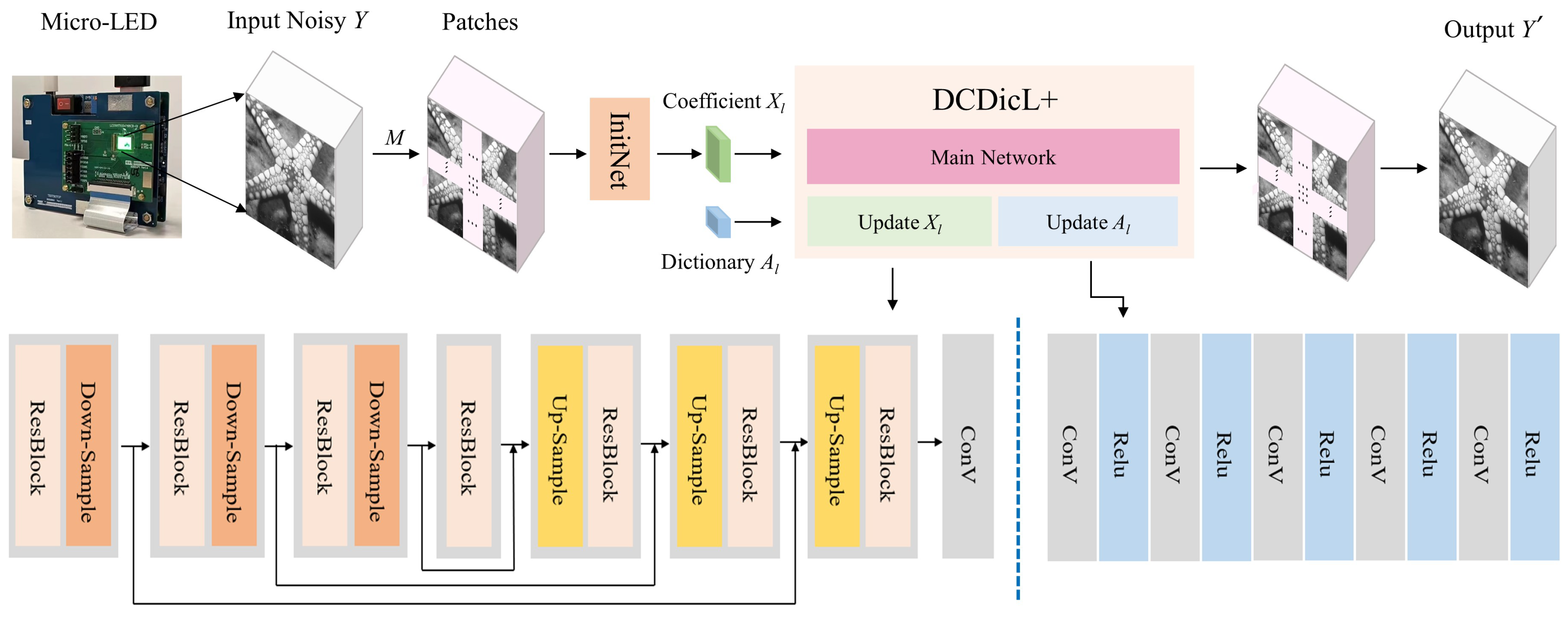
• Novel denoising method. An improved denoising method based on deep convolutional dictionary learning, where images are decomposed into small patches and adaptive dictionary learning is conducted, is proposed. This method provides a better representation of the fine structure of images, as both global and local features are incorporated, allowing for a more comprehensive representation of the fine structure present in images.
• Optimization algorithm. A new confidence-weighted fusion algorithm is developed to optimize the proposed method in our model; it can utilize the structures of the convolutional sparse coding structure, and local and global operators.
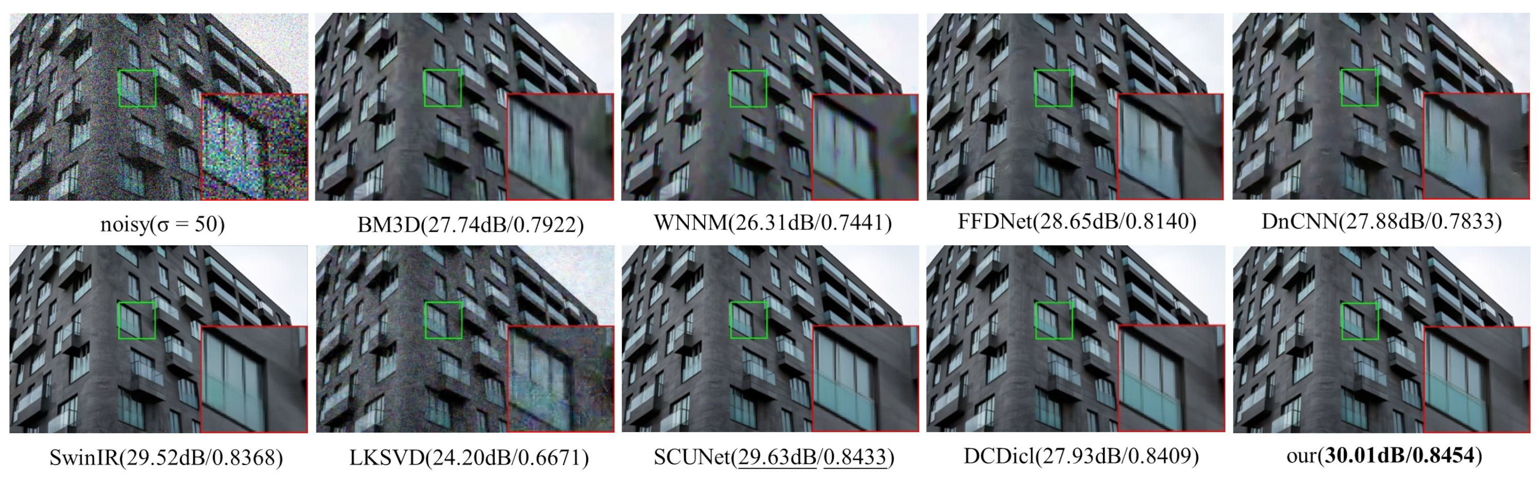
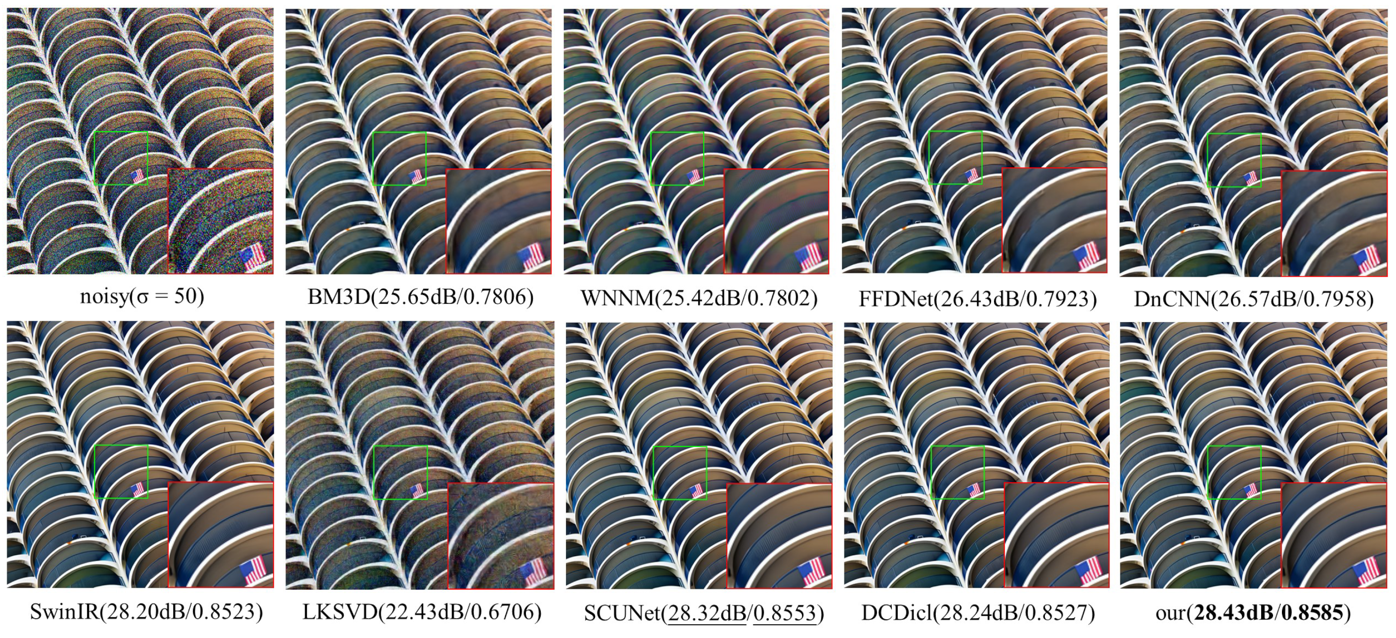
• Different applications. On the grayscale dataset Set12, compared with DCDicL, the PSNR and SSIM of the proposed method are increased by 3.87 dB and 0.0012 at the noise level of $\sigma =50$. On the color dataset Urban100, compared with DCDicL, the PSNR and SSIM of the proposed method are increased by 3.49 dB and 0.0133 at the noise level of $\sigma =50$.

The structure of this paper is as follows: Section 2 provides an extensive review of the relevant literature. In Section 3, we introduce our denoising method in detail. Comparative experiments demonstrating the effectiveness of the proposed denoising method are presented in Section 4. Finally, Section 5 summarizes the research results of this paper.

2. Related Works

2.1. Patch Denoising

Patch denoising is an image denoising method which eliminates or reduces noise around the modeling and processing of small patches in the image. The motivation behind patch denoising is to use the correlation between adjacent pixels in an image, aiming at restoring the real information of the image more accurately through the modeling of local patches. It is worth noting that the deep K-SVD (DK-SVD) method, which is integrated with deep learning, is an outstanding example in this category.

The DK-SVD method redesigns a learnable architecture based on K-SVD. Suppose that $x\in {\mathbb{R}}^{\sqrt{m}\times \sqrt{m}}$ is the input clean image patch. We define $\mathrm{x}=\mathrm{A}\alpha$, where $A\in {\mathbb{R}}^{m\times n}$ denotes a dictionary atom and $\alpha \in {\mathbb{R}}^n$ denotes the sparse vector. The noisy patch $y\in {\mathbb{R}}^{\sqrt{m}\times \sqrt{m}}$ is degraded by additive white Gaussian noise (AWGN) with standard deviation $\sigma$. Unlike K-SVD, DK-SVD uses the $l_1$-norm instead of the $l_0$-norm, replacing the greedy algorithm with the $l_1$-based iterative soft-thresholding algorithm (ISTA) [32]. This objective can be formulated as

$$\widehat{\alpha }=arg\underset{\alpha }{min}\frac{1}{2}{∥A\alpha -y∥}_2^2+\lambda {∥\alpha ∥}_1,$$

(1)

where $\lambda$ is the regularization coefficient and ${∥·∥}_1$ denotes the sum of the absolute values of the vector, which is the $l_1$-norm.

DK-SVD employs the iterative soft-thresholding algorithm (ISTA) to learn sparse matrix $\widehat{\alpha }$, which can be represented by the following iterative formula:

$${\widehat{\alpha }}_{k+1}=S_{\lambda /c}({\widehat{\alpha }}_k-\frac{1}{c}{A}^T(A{\widehat{\alpha }}_k-y));{\widehat{\alpha }}_0=0,$$

(2)

where k is the number of iterations, c denotes the square spectral norm of A, and $S_{\lambda /c}$ represents the soft-thresholding operator function.

$${\left[S_{\mu }\left(w\right)\right]}_i=\mathrm{s}gn\left(w_i\right){(\left|w_i\right|-\mu )}_{+},$$

(3)

As illustrated in Formula (3), by utilizing the proximal gradient descent approach, the sparse coding component is transformed into a trainable version. Performing operations on each patch of the image is essentially equivalent to convolving the image.

To control the error in a manageable way, a separate parameter, ${\lambda }_k$, is learned for each $y_k$. A multi-layer perceptron (MLP) network is utilized to learn a regression function, which maps inputs to outputs in the following manner: $\lambda =f_{\theta }\left(y\right)$, where $\theta$ represents the parameters of the MLP network.

During the patch reconstruction phase, the denoised image patch matrix ($\widehat{y}$) is obtained. Based on the already determined dictionary A and sparse vector $\widehat{\alpha }$, the denoised image patch can be reconstructed as follows: $\widehat{y}=A\widehat{\alpha }$, where A represents a set of learnable parameters. The entire patch denoising and patch reconstruction process is highly correlated with the convolutional sparse coding approach.

The complete end-to-end method architecture can be described as follows: The input image is segmented into fully overlapping patches at first; then, each corrupted patch is processed through the aforementioned patch denoising stage, and finally, the denoised versions of these patches are averaged to reconstruct the image. In the final step, the original K-SVD is abandoned, and a learnable method is designed to reconstruct the image. Let $u\in {\mathbb{R}}^{\sqrt{m}\times \sqrt{m}}$ be the weight coefficient for each patch; the reconstructed image is obtained by the following formula:

$$\widehat{X}=\frac{{\displaystyle \sum _k}{R}_k^T(u\odot {\widehat{\alpha }}_k)}{{\displaystyle \sum _k}{R}_k^{T}u},$$

(4)

where ⊙ is the Schur product. In the entire algorithm, the parameters that can be learned are $\theta$ (the vector of the parameters of the MLP), c (the step size in the ISTA), A (the dictionary), and u (the average weight of patches).

The main contribution of DK-SVD is to propose an end-to-end framework for deep learning methods. The framework retains the original computing path of K-SVD and redesigns a framework based on supervised learning. This architecture needs fewer learning parameters and retains the essence of K-SVD. Compared with the classical K-SVD method, its performance is significantly improved, and it is very close to the most advanced denoising method based on deep learning.

However, DK-SVD still uses fixed priors and adopts a generic dictionary rather than an image adaptive dictionary. In addition, the performance of the DK-SVD method is still behind that of many deep learning methods.

2.2. Convolutional Dictionary Learning

Convolutional dictionary learning denoising is a signal processing- and machine learning-based method employed for handling images contaminated by noise [34,35]. This method includes two key steps: dictionary learning and denoising processing.

In the initial stage, dictionary learning represents the first step of convolutional dictionary learning denoising. During this stage, the method endeavors to learn a set of fundamental structures or features from the input image, forming a dictionary. This dictionary encompasses convolutional kernels capable of efficiently representing the content of the image. The objective of dictionary learning is to compactly represent the input image, ensuring that the dictionary can effectively capture the local structures within the image.

Following the acquisition of the dictionary, the input image can undergo sparse representation using the dictionary. Sparse representation means that the image can be represented as a linear combination of several bases in a dictionary, thus producing a more concise representation. Through sparse representation, the basic structures of the image can be extracted, and the noise is represented by a small coefficients.

The noise in the sparse representation coefficients can be effectively reduced by convolutional denoising. In this step, convolutional kernels are employed to filter the sparse representation coefficients, eliminating noise components. Finally, through inverse sparse coding and inverse convolutional operations, the denoised coefficients are restored to the ultimate denoised image. Suppose that $Y_i\in {\mathbb{R}}^{h\times w}$ is the i-th training sample; the objective function can be written as follows:

$$\underset{A,\left\{X_i\right\}}{min}\frac{1}{N}\sum _{i=1}^N\frac{1}{2}{∥A\otimes X_i-Y_i∥}_2^2+{\lambda }_X\psi \left(X_i\right)+{\lambda }_A\varphi \left(A\right),$$

(5)

where $A\otimes X_i={\displaystyle \sum _{c=1}^C}{A}_c\ast X_{i,c}$, ∗ is the two-dimensional convolutional operation, C is the number of channels, A represents the convolutional dictionary, $X_i={\left\{X_{i,c}\right\}}_{c=1}^C$ is the sparse feature map of image $Y_i$, ${\lambda }_{X_i}$ and ${\lambda }_A$ are penalty parameters for $X_i$ and A, $\psi \left(X_i\right)$ denotes the prior distribution of input variable $X_i$, and $\varphi \left(A\right)$ is a regularization term for dictionary A.

Based on the learning method of convolutional dictionary mentioned above, Zheng et al. [33] proposed an improved deep convolutional dictionary learning (DCDicL) method. This method not only learns the deep prior of coefficient X but also learns the deep prior of convolutional dictionary A from the training data, and provides an adaptive dictionary for each image. The learning process can be expressed by the following formula:

$$\underset{\{A_i,X_i\}}{min}\frac{1}{N}\sum _{i=1}^N\frac{1}{2}{∥A_i\otimes X_i-Y_i∥}_2^2+{\lambda }_X\psi \left(X_i\right)+{\lambda }_A\varphi \left(A_i\right),$$

(6)

The expression above can be rewritten as the following optimization problem:

$$\begin{array}{cc}\hfill & min\frac{1}{N}\sum _{i=1}^{N}F(A_i\otimes X_i,Y_i^{gt})\hfill \\ \hfill \mathrm{s}.\mathrm{t}.M\{A_i,X_i\}& =arg\underset{A,X}{min}\frac{1}{2{\sigma }_i^2}{∥A\otimes X-Y_i∥}_2^2+{\lambda }_X\psi \left(X\right)+{\lambda }_A\varphi \left(A\right),\hfill \end{array}$$

(7)

where $Y_i^{gt}$ is the ground truth version of $Y_i$, $F(,)$ is a function for measuring loss, and ${\sigma }_i$ represents the level of noise.

DCDicL strictly follows the mathematical formula of dictionary learning, learning the prior knowledge of X and A from training data, and learning a specific dictionary for each image. The dictionary can adapt to the image content and perceive the global information, thus giving DCDicL a powerful ability to recover the fine image structures even under severe noise. However, the DCDicL denoising method still cannot represent the fine structure of images very well, and its performance still needs to be improved.

3. Methodology

3.1. Proposed Method

Inspired by the related work, we put forward a deep convolutional dictionary learning denoising method based on distributed image patches (DCDicL+). This method not only processes the images globally but also processes the segmented image patches locally through similar patches. The proposed method enhances the restoration of fine details in the images. The fundamental method can be expressed as a minimization problem with the following formula:

$$\begin{array}{c}\hfill \underset{A,X}{min}\left\{\frac{1}{2}{∥A\otimes X-Y∥}_F^2+{\lambda }_1\psi \left(X\right)+{\lambda }_2\phi \left(A\right)\right\}.\end{array}$$

(8)

In this method, the complete noisy image is represented by Y, the global image dictionary is denoted by A, and X is introduced as the sparse coefficient.

3.2. Optimization Algorithm

Convolutional dictionary learning decomposes the entire image using convolutional operations, reducing redundancy in patch representations. Patch denoising helps preserve more details in the image. To obtain an effective method, Equation (8) is rewritten in the following forms of problems:

$$\begin{array}{cc}\hfill & \underset{\left\{A_l,X_l\right\}}{min}\left\{\sum _{l=1}^d\frac{1}{2}{∥A_l\otimes X_l-Y_l∥}_F^2+{\lambda }_1\psi \left(X_l\right)+{\lambda }_2\varphi \left(A_l\right)\right\},\hfill \\ \hfill & \mathrm{s}.\mathrm{t}.A_l\otimes X_l\in M,\hfill \end{array}$$

(9)

where M is the given global constraint, ${\lambda }_1$ and ${\lambda }_2$ are penalty parameters for $X_l$ and $A_l$, $\psi \left(X_l\right)$ denotes the prior distribution of input variable $X_l$, and $\varphi \left(A_l\right)$ is a regularization term for dictionary $A_l$. By introducing auxiliary variables ${X_l}^{\prime }$ and ${A_l}^{\prime }$ to incorporate the denoising prior, Equation (9) can be expressed as

$$\begin{array}{cc}\hfill & \underset{X_l,{X_l}^{\prime }}{min}\left\{\frac{1}{2}{∥A_l\otimes {X_l}^{\prime }-Y_l∥}_F^2+{\lambda }_1\psi \left(X_l\right)\right\},\hfill \\ \hfill & \mathrm{s}.\mathrm{t}.X_l={X_l}^{\prime },A_l\otimes X_l\in M.\hfill \end{array}$$

(10)

$$\begin{array}{cc}\hfill & \underset{A_l,{A_l}^{\prime }}{min}\left\{\frac{1}{2}{∥{A_l}^{\prime }\otimes X_l-Y_l∥}_F^2+{\lambda }_2\varphi \left(A_l\right)\right\},\hfill \\ \hfill & \mathrm{s}.\mathrm{t}.A_l={A_l}^{\prime },A_l\otimes X_l\in M.\hfill \end{array}$$

(11)

The constrained optimization problem above can be solved by using the half quadratic splitting (HQS) method [36]; then, the optimization problems are equivalent to minimizing the following two formulas:

$$\begin{array}{cc}\hfill & \underset{X_l,{X_l}^{\prime }}{min}\left\{\frac{1}{2}{∥A_l\otimes {X_l}^{\prime }-Y_l∥}_F^2+{\lambda }_1\psi \left(X_l\right)+\frac{{\mu }_X}{2}{∥X_l-{X_l}^{\prime }∥}_F^2\right\},\hfill \\ \hfill & \mathrm{s}.\mathrm{t}.A_l\otimes X_l\in M.\hfill \end{array}$$

(12)

$$\begin{array}{cc}\hfill & \underset{A_l,{A_l}^{\prime }}{min}\left\{\frac{1}{2}{∥{A_l}^{\prime }\otimes X_l-Y_l∥}_F^2+{\lambda }_2\varphi \left(A_l\right)+\frac{{\mu }_A}{2}{∥A_l-{A_l}^{\prime }∥}_F^2\right\},\hfill \\ \hfill & \mathrm{s}.\mathrm{t}.,A_l\otimes X_l\in M,\hfill \end{array}$$

(13)

where ${\mu }_X$ and ${\mu }_A$ are penalty parameters. The above equations can be solved iteratively, and auxiliary variables ${X_l}^{\mathrm{\Theta }}$ and ${A_l}^{\mathrm{\Theta }}$ are introduced in the following formulas. For the update of sparse coefficient $X_l$, Equation (12) can be resolved by alternately optimizing the following subproblems:

$$\begin{array}{cc}\hfill {X_{l,\left(t\right)}}^{\prime }& =arg\underset{{X_l}^{\mathrm{\Theta }}}{min}\left\{\frac{1}{2}{∥A_{l,(t-1)}\otimes {X_l}^{\mathrm{\Theta }}-Y_l∥}_F^2+\frac{{\beta }_X}{2}{∥{X_l}^{\mathrm{\Theta }}-{X_l}_{,(t-1)}∥}_F^2\right\}\hfill \\ \hfill & =\frac{1}{{\beta }_X}{F}^{-1}\left\{\left(a\circ y_{\uparrow C}+{\beta }_{X}x\right)-a\circ \left[\frac{\overline{a}\odot \left(a\circ y_{\uparrow C}+{\beta }_{X}x\right)}{{\alpha }_1+\left(\overline{a}\odot a\right)}{\uparrow }_C\right]\right\},\hfill \\ \hfill \mathrm{s}.\mathrm{t}.& {\beta }_X={\mu }_X{\sigma }^2,y=F\left(Y_l\right),a=F\left(A_l\right),x=F\left(X_l\right),A_l\otimes X_l\in M.\hfill \end{array}$$

(14)

$$\begin{array}{cc}\hfill X_{l,\left(t\right)}& =arg\underset{{X_l}^{\mathrm{\Theta }}}{min}\left\{\psi \left({X_l}^{\mathrm{\Theta }}\right)+\frac{{\omega }_X}{2}{∥{X_{l,\left(t\right)}}^{\prime }-{X_l}^{\mathrm{\Theta }}∥}_F^2\right\}\hfill \\ \hfill & =prior\left({X_{l,\left(t-1\right)}}^{\prime }\right),\hfill \\ \hfill \mathrm{s}.\mathrm{t}.& {\omega }_X={\mu }_X/\phantom{{\mu }_X{\lambda }_1}{\lambda }_1,A_l\otimes X_l\in M,\hfill \end{array}$$

(15)

where $\sigma$ represents the noise level of the image patch and t denotes the number of iterations. Equation (14) obtains a closed-form solution for $X_{l,\left(t\right)}$ through fast Fourier transform (FFT) [37]. $F\left(\right)$ and $F^{-1}\left(\right)$ represent 2D FFT and its corresponding inverse transform, respectively. As a common operation in neural networks, the convolutional operation in the equations is typically implemented through matrix multiplication. ∘ is the Hadamard product. ${\uparrow }_C$ expands the channel dimension. $\overline{d}\odot d={\sum }_{C=1}^C{{\overline{d}}_C\circ d}_C$. Equation (15) is updated through a neural network for the variables. $prior\left(\right)$ represents the nonlinear mapping of the neural network. The prior knowledge of sparse coefficients $X_l$ is learned through a U-Net structure [38]. For hyperparameters ${\beta }_X$ and ${\omega }_X$, we employ a configuration consisting of two Conv layers followed by a SoftPlus layer with input $\sigma$ to predict the hyperparameters for each stage. For updating dictionary $A_l$, Equation (13) can be reformulated as the following subproblem:

$$\begin{array}{cc}\hfill {A_{l,\left(t\right)}}^{\prime }& =arg\underset{{A_l}^{\mathrm{\Theta }}}{min}\left\{\frac{1}{2}{∥{A_l}^{\mathrm{\Theta }}\otimes {X_{l,}}_{\left(t\right)}-Y_l∥}_F^2+\frac{{\beta }_A}{2}{∥{A_l}^{\mathrm{\Theta }}-{A_l}_{,(t-1)}∥}_F^2\right\}\hfill \\ \hfill & =ve{c}^{-1}\left\{{\left({\mathrm{X}}^T\mathrm{X}+{\beta }_{A}I\right)}^{-1}\left({\mathrm{X}}^T{\rm Y}+{\beta }_A\mathrm{A}\right)\right\},\hfill \\ \hfill \mathrm{s}.\mathrm{t}.& {\beta }_A={\mu }_A{\sigma }^2,\mathrm{A}=ve{c}^{-1}\left(A_l\right).\hfill \end{array}$$

(16)

$$\begin{array}{cc}\hfill A_{l,\left(t\right)}& =arg\underset{{A_l}^{\mathrm{\Theta }}}{min}\left\{\varphi \left({A_l}^{\mathrm{\Theta }}\right)+\frac{{\omega }_A}{2}{∥A_l{{ }_{,\left(t\right)}}^{\prime }-{A_l}^{\mathrm{\Theta }}∥}_F^2\right\}\hfill \\ \hfill & =prior\left({A_{l,\left(t-1\right)}}^{\prime }\right),\hfill \\ \hfill \mathrm{s}.\mathrm{t}.& {\omega }_A={\mu }_A/\phantom{{\mu }_A{\lambda }_2}{\lambda }_2,A_l\otimes X_l\in M,\hfill \end{array}$$

(17)

where $vec\left(\right)$ is the vectorization operator and $ve{c}^{-1}\left(\right)$ reverses the vectorization. $\mathrm{X}$, ${\rm Y}$, and $\mathrm{A}$ denote the dimensional transformation results of matrices $X_l$, $Y_l$, and $A_l$, respectively. The convolutional multiplication in Equation (16) is expanded into matrix multiplication, and the solution for $A_{l,\left(t\right)}$ is obtained using the least squares method. Furthermore, Equation (17) is updated through a shallower neural network. Prior knowledge on dictionary $A_l$ is learned through a relatively shallow network, consisting of six Conv layers with ReLU activation. For hyperparameters ${\beta }_A$ and ${\omega }_A$, we employ a configuration consisting of two Conv layers followed by a SoftPlus layer [39] with input $\sigma$ to predict the hyperparameters for each stage. For updating global parameter M, by introducing auxiliary variables $M^{\prime }$ to incorporate the global denoising prior, the problem can be reformulated as the following formulas:

$$\begin{array}{c}\hfill {M_{\left(t\right)}}^{\prime }={M_{(t-1)}}^{\prime }-{\alpha }_M{\mu }_M({M_{(t-1)}}^{\prime }-M_{(t-1)}).\end{array}$$

(18)

$$\begin{array}{c}\hfill M_{\left(t\right)}=M_{(t-1)}-{\alpha }_M\nabla f\left(M_{(t-1)}\right),\end{array}$$

(19)

where ${\alpha }_M$ represents the learning rate and ∇ denotes the gradient. Specifically, $\nabla f\left(M_{\left(t\right)}\right)$ represents the gradient of the objective function ($f\left(M\right)$) with respect to variable M at iteration t. The output image patch can be obtained through convolutional multiplication:

$$\begin{array}{c}\hfill {Y_{l,\left(t\right)}}^{\prime }=A_{l,\left(t\right)}\otimes X_{l,\left(t\right)}\end{array}$$

(20)

3.3. Confidence-Weighted Fusion of Image Patches

The denoised image patches processed as mentioned above are combined into a complete output image according to specified offsets. Initially, a confidence matrix is generated by calculating the probability density values for each point in the image patches. Subsequently, the final denoised image is obtained by weighted summation of confidence-weighted input image patches. This approach ensures the preservation of high-confidence information and can be expressed as

$$\begin{array}{c}\hfill P\left({Y_{l,\left(t\right)}}^{\prime }\right)=\frac{exp\left(-\frac{1}{2}{\left({Y_{l,\left(t\right)}}^{\prime }-\alpha \right)}^T{\mathrm{\Sigma }}^{-1}\left({Y_{l,\left(t\right)}}^{\prime }-\alpha \right)+\tau M\right)}{{\sqrt{\left(2\pi \right)}}^{k}det\mathrm{\Sigma }},\end{array}$$

(21)

$$\begin{array}{c}\hfill Y^{\prime }=\left\{\begin{array}{c}{\displaystyle \sum _t}\left[P\left({Y_{1,\left(t\right)}}^{\prime }\right)\times {Y_{1,\left(t\right)}}^{\prime }\right],\hfill \\ {\displaystyle \sum _t}\left[P\left({Y_{2,\left(t\right)}}^{\prime }\right)\times {Y_{2,\left(t\right)}}^{\prime }\right],\hfill \\ ...,{\displaystyle \sum _t}\left[P\left({Y_{d,\left(t\right)}}^{\prime }\right)\times {Y_{d,\left(t\right)}}^{\prime }\right]\hfill \end{array}\right\},\end{array}$$

(22)

where $P\left(\right)$ denotes the probability density function of a multivariate Gaussian distribution, ${Y_l}^{\prime }$ is the image patch processed after denoising, $Y^{\prime }$ is the fully assembled denoised image, $\tau$ represents the penalty term for the global component, ∑ represents the covariance matrix, $det\sum$ is the determinant of ∑, k is the dimensionality, and $\alpha$ denotes the mean.

In conclusion, the solution steps of the method proposed in this paper are shown in Algorithm 1. More specifically, InitNet, consisting of two Conv layers with ReLU activation, is employed to learn initialization coefficient $X_{l,\left(0\right)}$. Subsequently, for each of the t iterations, the value of ${X_{l,\left(t\right)}}^{\prime }$ is calculated by Equation (14). This result is then fed into Equation (15), which includes three connected up-sampling blocks and three down-sampling blocks, allowing for the estimation of the sparse coefficient by using the prior learned from the training data. Similar procedures are applied for updating dictionary $A_{l,\left(t\right)}$ and $M_{\left(t\right)}$. The final image is obtained through convolutional operation and confidence fusion.

The effectiveness of our proposed method will be analyzed in the experimental part of Section 4.

Algorithm 1: DCDicL+

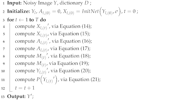
4. Experimental Results

In this section, we report the experimental results. The training data were generated by using the WED [40] (4744 images), DIV2K [41] (900 images), and BSD400 [42] (400 images) datasets. The tests were conducted on the grayscale datasets Set12 (12 images), BSD68 [43] (68 images), and Urban100 [44] (100 images) and the color datasets Urban100 [44] (100 images), CBSD48 [43] (48 images), and Kodak24 [45] (24 images). All experiments were carried out on the GTX 1080Ti GPU with CUDA version 11.2 using PyTorch.

Peak signal-to-noise ratio (PSNR) [46] and structural similarity (SSIM) [47] were employed for assessing the local consistency within image patches. Additionally, the consistency between different local regions was evaluated with the mean square error (MSE) [48]. For the given clean image $Y^{\prime }$ and noisy image Y with a size of $m\times n$, MSE is defined as follows:

$$\begin{array}{c}\hfill MSE=\frac{1}{\mathrm{mn}}\sum _{i=0}^{m-1}\sum _{j=0}^{n-1}{\left[Y^{\prime }\left(i,j\right)-Y\left(i,j\right)\right]}^2\end{array},$$

where the PSNR value is contingent on the MSE, implying that a smaller MSE corresponds to a higher PSNR value. This relationship indicates a diminished distinction between the reconstructed image and the actual image. PSNR is defined as

$$\begin{array}{c}\hfill PSNR=10·{log}_{10}\left(\frac{MA{X}^2}{MSE}\right)\end{array},$$

where $MAX$ represents the maximum pixel value of the image. In parallel, SSIM serves as a metric for gauging the likeness between the reconstructed and actual images in dimensions such as brightness, contrast, and structure. SSIM can be mathematically formulated as follows:

$$\begin{array}{c}\hfill SSIM=\frac{\left(2{\mu }_{Y^{\prime }}{\mu }_Y+c_1\right)\left(2{\sigma }_{Y^{\prime }Y}+c_2\right)}{\left({\mu }_{Y^{\prime }}^2+{\mu }_Y^2+c_1\right)\left({\epsilon }_{Y^{\prime }}^2+{\epsilon }_Y^2+c_2\right)},\end{array}$$

where ${\sigma }_{Y^{\prime }Y}$ is the covariance between the reconstructed and original images, ${\mu }_{Y^{\prime }}$ and ${\mu }_Y$ represent the means, ${\epsilon }_{Y^{\prime }}$ and ${\epsilon }_Y$ represent the variance, and $c_1$ and $c_2$ are constants. A greater SSIM value denotes heightened similarity between the two images, signifying superior image quality.

4.1. Parameter Settings

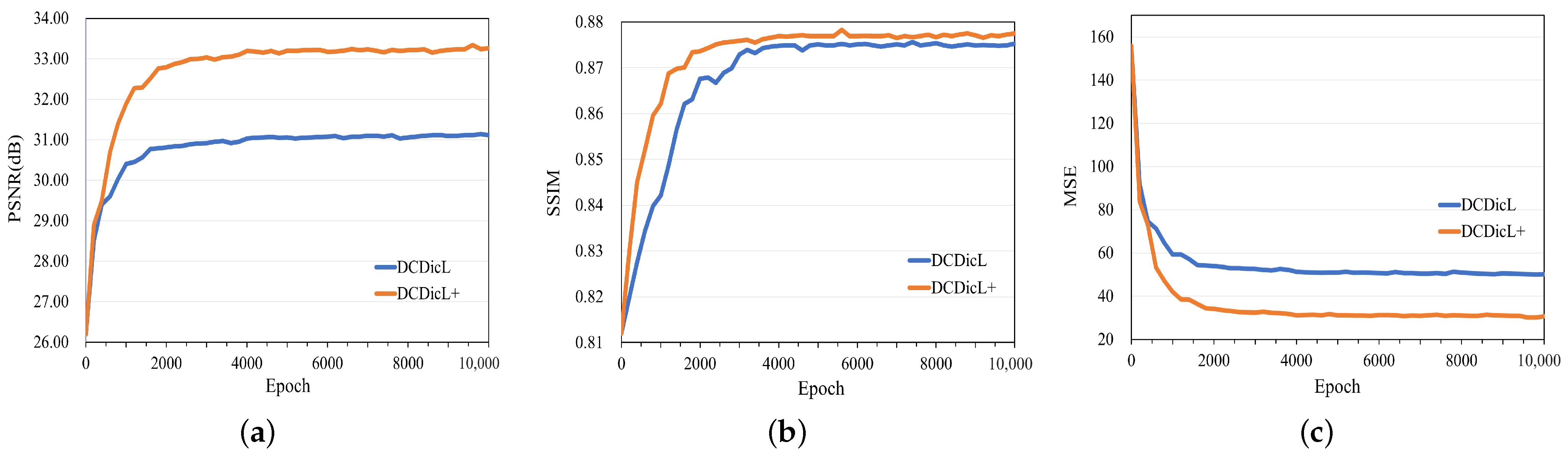
4.1.1. Training Iterations

For each input image, the image patch size was set to $128\times 128$, and the confidence merging step size was set to 8. During the training process, Gaussian noise with zero average value and a noise level in the range of $\sigma \in [0,50]$ was added to the images. These noisy images were trained in batches. The learning rate was set to ${10}^{-4}$, and the batch size was set to 16 on the GTX 1080Ti GPU. The loss function utilized $L_1$ loss, and the Adam optimizer [49] was employed for updating the network parameters. Iteration T was carried out in four stages, which are discussed in Section 4.3. The number of atoms in dictionary A was fixed at 64, and the size of A was set to 5. Simultaneously, to ensure the convergence of the training function, this study employed a self-constructed dataset for validation. Figure 2a,b illustrate the changes in PSNR (dB) and SSIM with the increase in training iterations when the noise level is $\sigma =25$. Figure 2c illustrates the changes in MSE with the increase in training iterations. It can be observed that with a greater number of iterations, the values of PSNR and SSIM gradually improve, and MSE gradually converges. After 4000 iterations, a favorable outcome is achieved, prompting the decision to establish the final number of iterations at 4000.

Figure 2. Contrast curves of noise level of $\sigma =25$ during training. (a) PSNR (dB) trends of DCDicL and DCDicL+, (b) SSIM trends of DCDicL and DCDicL+, and (c) MSE trends of DCDicL and DCDicL+.

4.1.2. Confidence Scaling Factor

Different values of confidence scaling factor p produce different regions of interest, potentially resulting in excessive smoothing or loss of local detail information in the image. Parameter p controls the size of the covariance matrix for confidence-weighted multivariate normal distributions, influencing the spatial range of the multivariate normal distribution around the center of the image patch and consequently affecting the confidence distribution of each pixel. A larger p value leads to a wider confidence distribution, exerting a greater impact on surrounding pixels during the mosaic process, whereas a smaller p value results in a more localized confidence distribution.

To assess the influence of different confidence scaling factors, this study additionally performed ablation analysis by varying the scaling factor (p), demonstrating that $p=2$ is the optimal parameter selection. Moreover, it was observed that further increases in p did not significantly enhance performance. Further details can be found in Section 4.3. The experimental results are shown in Table 1 and Table 2 (where the bold values represent the best values).

Table 1. Comparison of PSNR (dB)/SSIM average values with different scaling factors on grayscale datasets.

Dataset		Noise	$\mathit{p}=0.5$	$\mathit{p}=2$
Set12		15	34.45/0.9142	34.45/$\mathbf{0}.\mathbf{9143}$
		25	33.17/0.8765	$\mathbf{33}.\mathbf{19}/\mathbf{0}.\mathbf{8769}$
		50	31.25/0.8109	$\mathbf{31}.\mathbf{87}/\mathbf{0}.\mathbf{8116}$
BSD68		15	32.14/0.9136	32.14/$\mathbf{0}.\mathbf{9137}$
		25	31.15/0.8577	$\mathbf{31}.\mathbf{16}/\mathbf{0}.\mathbf{8579}$
		50	30.23/0.7292	$\mathbf{30}.\mathbf{25}/\mathbf{0}.\mathbf{7295}$
Urban100		15	33.42/0.9472	$\mathbf{33}.\mathbf{43}/\mathbf{0}.\mathbf{9473}$
		25	32.20/0.9179	$\mathbf{32}.\mathbf{22}/\mathbf{0}.\mathbf{9182}$
		50	30.93/0.8556	$\mathbf{30}.\mathbf{96}/\mathbf{0}.\mathbf{8562}$

Table 2. Comparison of PSNR (dB)/SSIM average values with different scaling factors on color datasets.

Dataset		Noise	$\mathit{p}=0.5$	$\mathit{p}=2$
Set12		15	34.45/0.9142	34.45/$\mathbf{0}.\mathbf{9143}$
		25	34.16/0.9460	$\mathbf{34}.\mathbf{18}/\mathbf{0}.\mathbf{9462}$
		50	32.46/0.9014	$\mathbf{32}.\mathbf{48}/\mathbf{0}.\mathbf{9017}$
CBSD68		15	34.90/0.9381	$\mathbf{34}.\mathbf{91}$/0.9381
		25	33.32/0.8976	$\mathbf{33}.\mathbf{34}/\mathbf{0}.\mathbf{8977}$
		50	31.94/0.8156	$\mathbf{31}.\mathbf{96}/\mathbf{0}.\mathbf{8159}$
Kodak24		15	35.70/0.9316	$\mathbf{35}.\mathbf{71}/\mathbf{0}.\mathbf{9317}$
		25	34.11/0.8947	$\mathbf{34}.\mathbf{13}/\mathbf{0}.\mathbf{8949}$
		50	32.63/0.8230	$\mathbf{32}.\mathbf{64}/\mathbf{0}.\mathbf{8233}$

Compared with $p=0.5$ for original input images with noise levels of $\sigma =15,25,$ and 50 in the grayscale dataset Urban100, using $p=2$ for denoising can increase the PSNR by 0.01 dB, 0.02 dB, and 0.03 dB and SSIM by 0.0001, 0.0003, and 0.0006, respectively. In the color dataset Urban100, compared with $p=0.5$, using $p=2$ for denoising can increase the PSNR by 0.01 dB, 0.02 dB, and 0.02 dB and SSIM by 0.0002, 0.0002, and 0.0003, respectively. The experiments indicate that when the scale factor (p) is set to 2, the values of the PSNR and SSIM are better, so $p=2$ was set in subsequent experiments.

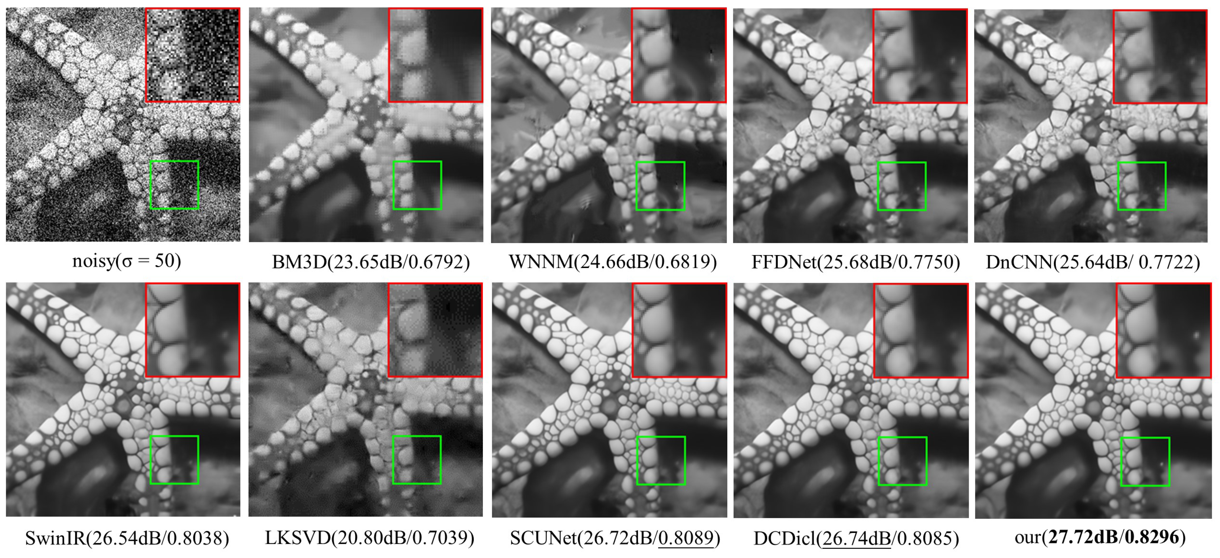
4.2. Comparison Results

In order to verify the proposed denoising method, DCDicL+, noise levels of 15, 25, and 50 were added to the original input images. DCDicL+ was compared with several representative denoising methods, including BM3D [20], WNNM [23], FFDNet [27], DnCNN [18], SwinIR [45], LKSVD [31], DCDicL [33], and SCUNet [47]. The implementation codes of these comparison methods are provided by their respective authors (https://github.com/natezhenghy/DCDicL_denoising, accessed on 17 December 2023) and tested on the same datasets.

4.2.1. Grayscale Datasets

As shown in Table 3, the best PSNR and SSIM for each noise level in each dataset are displayed in bold, indicating the best results, and those underlined indicate the second best results. It can be observed that compared with other denoising methods, the proposed denoising method achieves superior performance on the grayscale datasets Set12, BSD68, and Urban100. The improvement range for the PSNR is 0.15 dB to 11.03 dB, and the improvement range for SSIM is 0.0002 to 0.1851. On the dataset Set12, compared with DCDicL, the PSNR/SSIM of the proposed method are increased by 1.11 dB/0.0028, 2.16 dB/0.0021, and 3.87 dB/0.0012, respectively; Compared with SCUNet, they are increased by 1.02 dB/0.0126, 2.10 dB/0.0015, and 3.83 dB/0.0002, respectively. This can be attributed to the excellent learning capability of DCDicL+ with a large number of training data. The proposed method explores the inherent characteristics in images and performs finer denoising and restoration of the fine structure in the images.

Table 3. Comparison of PSNR (dB)/SSIM average values on different grayscale datasets.

	Dataset	Set12			BSD68			Urban100
Method		$\mathbf{\sigma }=\mathbf{15}$	$\mathbf{\sigma }=\mathbf{25}$	$\mathbf{\sigma }=\mathbf{50}$	$\mathbf{\sigma }=\mathbf{15}$	$\mathbf{\sigma }=\mathbf{25}$	$\mathbf{\sigma }=\mathbf{50}$	$\mathbf{\sigma }=\mathbf{15}$	$\mathbf{\sigma }=\mathbf{25}$	$\mathbf{\sigma }=\mathbf{50}$
BM3D		32.37/	29.97/	26.72/	31.07/	28.57/	25.60/	32.35/	29.70/	25.95/
		0.8952	0.8504	0.7676	0.8717	0.8013	0.6864	0.9220	0.8777	0.7791
WNNM		32.71/	30.26/	27.05/	31.37/	28.83/	25.87/	32.53/	30.38/	26.83/
		0.8988	0.8557	0.7775	0.8766	0.8087	0.6982	0.9271	0.8885	0.8047
FFDNet		32.75/	30.43/	27.32/	31.63/	29.19/	26.29/	32.40/	29.90/	26.50/
		0.9024	0.8631	0.7899	0.8902	0.8288	0.7239	0.9265	0.8979	0.8048
DnCNN		32.86/	30.44/	27.18/	31.73/	29.23/	26.23/	32.64/	29.95/	26.26/
		0.9024	0.8617	0.7828	0.8907	0.8279	0.7189	0.9246	0.8781	0.7856
SwinIR		33.36/	31.01/	27.91/	31.97/	29.50/	26.58/	32.70/	31.30/	27.98/
		0.8898	0.8482	0.8119	0.8959	0.8321	0.7298	0.9104	0.8724	0.8039
LKSVD		28.72/	24.85/	20.84/0	28.48/	24.96/	20.97/	28.46/	23.80/	20.22/
		0.7826	0.7354	0.7042	0.7835	0.7371	0.7035	0.7836	0.7331	0.7018
DCDicL		33.34/	31.03/	28.00/	31.95/	29.52/	26.63/	32.31/	29.65/	26.22/
		0.9115	0.8748	0.8122	0.8957	0.8379	0.7395	0.9383	0.9129	0.8336
SCUNet		33.43/	31.09/	28.04/	31.99/	29.55/	26.67/	32.88/	31.58/	28.56/
		0.9017	0.8754	0.8132	0.9001	0.8402	0.7456	0.9458	31.58/	0.8392
Our		$\mathbf{34}.\mathbf{45}/$	$\mathbf{33}.\mathbf{19}/$	$\mathbf{31}.\mathbf{87}/$	$\mathbf{32}.\mathbf{14}/$	$\mathbf{31}.\mathbf{16}/$	$\mathbf{30}.\mathbf{25}/$	$\mathbf{33}.\mathbf{43}/$	$\mathbf{32}.\mathbf{22}/$	$\mathbf{30}.\mathbf{96}/$
		$\mathbf{0}.\mathbf{9143}$	$\mathbf{0}.\mathbf{8769}$	$\mathbf{0}.\mathbf{8134}$	$\mathbf{0}.\mathbf{9137}$	$\mathbf{0}.\mathbf{8579}$	$\mathbf{0}.\mathbf{7478}$	$\mathbf{0}.\mathbf{9473}$	$\mathbf{0}.\mathbf{9182}$	$\mathbf{0}.\mathbf{8562}$

Simultaneously, this paper selected two images from Set12 and introduced Gaussian noise at the level of $\sigma =50$ to further validate the visual denoising effect. The experimental results are shown in Figure 3 and Figure 4. The green boxes are enlarged images of the red boxes. Upon closer inspection of the enlarged comparison diagrams, it becomes evident that DCDicL+ restores more edge and texture information. According to the analysis of specific numerical values, the proposed method demonstrates significant improvement compared with other methods on the image Starfish, exhibiting enhancements ranging from 0.98 dB to 6.92 dB in the PSNR and improvements from 0.0207 to 0.1504 in SSIM. Likewise, on the image House, the proposed method exhibits clear superiority over other methods, manifesting improvements in the PSNR from 2.57 dB to 12.59 dB and enhancements in SSIM from 0.0308 to 0.1007.

Figure 3. Grayscale image Starfish with noise level $\sigma =50$: results of different methods (PSNR (dB)/SSIM).

Figure 4. Grayscale image House with noise level $\sigma =50$: results of different methods (PSNR (dB)/SSIM).

4.2.2. Color Datasets

For the color datasets Urban100, CBSD68, and Kodak24, Table 4 provides a comparative analysis of various methods based on the PSNR and SSIM. Compared with DCDicL, the PSNR/SSIM of the proposed method are improved by 0.91 dB/0.0149, 1.41 dB/0.0162, and 3.49 dB/0.0133, respectively, on the color dataset Urban100. Compared with SCUNet, these performance metrics are improved by 0.63 dB/0.0107, 1.15 dB/0.0120, and 2.34 dB/0.0116, respectively. It can be observed that the proposed method also demonstrates effective denoising performance on color images and restores them effectively.

Table 4. Comparison of PSNR (dB)/SSIM average values on different color datasets.

	Dataset	Urban100			CBSD68			Kodak24
Method		$\mathbf{\sigma }=\mathbf{15}$	$\mathbf{\sigma }=\mathbf{25}$	$\mathbf{\sigma }=\mathbf{50}$	$\mathbf{\sigma }=\mathbf{15}$	$\mathbf{\sigma }=\mathbf{25}$	$\mathbf{\sigma }=\mathbf{50}$	$\mathbf{\sigma }=\mathbf{15}$	$\mathbf{\sigma }=\mathbf{25}$	$\mathbf{\sigma }=\mathbf{50}$
BM3D		33.93/	31.36/	27.93/	33.50/	30.69/	27.36/	34.26/	31.67/	28.44/
		0.9408	0.9092	27.93/	0.9215	0.8672	0.7626	0.9147	0.8670	0.7760
WNNM		32.86/	32.86/	27.18/	31.73/	31.73/	26.23/	32.64/	29.95/	26.26/
		0.9024	0.9024	0.7828	0.8907	0.8907	0.7189	0.9246	0.8781	0.7856
FFDNet		33.83/	31.40/	28.05/	33.87/	31.21/	27.96/	34.63/	32.13/	28.98/
		0.9418	0.9120	0.8476	0.9290	0.8821	0.7887	0.9224	0.8791	0.7952
DnCNN		32.98/	30.81/	27.59/	33.89/	31.23/	27.92/	34.48/	32.03/	28.85/
		0.9314	0.9015	0.8331	0.9290	0.8830	0.7896	0.9209	0.8775	0.7917
SwinIR		35.13/	32.90/	29.82/	34.42/	31.78/	28.56/	35.34/	32.89/	29.79/
		0.9532	0.9284	0.8675	0.9203	0.8862	0.7890	0.9212	0.8864	0.8041
LKSVD		32.76/	30.37/	27.12/	31.63/	29.15/	26.19/	32.46/	29.80/	26.22/
		0.8106	0.7798	0.7187	0.8282	0.7848	0.7169	0.8236	0.7831	0.7318
DCDicL		34.90/	32.77/	28.99/	34.36/	31.75/	28.57/	35.38/	32.97/	29.96/
		0.9511	0.9300	0.8884	0.9348	0.8930	0.8107	0.9300	0.8928	0.8219
SCUNet		35.18/	33.03/	30.14/	34.40/	31.79/	28.61/	35.34/	32.92/	29.87/
		0.9553	0.9342	0.8901	0.9351	0.8931	0.8130	0.9293	0.8922	0.8198
Our		$\mathbf{35}.\mathbf{81}/$	$\mathbf{34}.\mathbf{18}/$	$\mathbf{32}.\mathbf{48}/$	$\mathbf{34}.\mathbf{91}/$	$\mathbf{33}.\mathbf{34}/$	$\mathbf{31}.\mathbf{96}/$	$\mathbf{35}.\mathbf{71}/$	$\mathbf{34}.\mathbf{13}/$	$\mathbf{32}.\mathbf{64}/$
		$\mathbf{0}.\mathbf{9660}$	$\mathbf{0}.\mathbf{9462}$	$\mathbf{0}.\mathbf{9017}$	$\mathbf{0}.\mathbf{9381}$	$\mathbf{0}.\mathbf{8977}$	$\mathbf{0}.\mathbf{8159}$	$\mathbf{0}.\mathbf{9317}$	$\mathbf{0}.\mathbf{8949}$	$\mathbf{0}.\mathbf{8233}$

Similarly, from the visual representation in Figure 5 and Figure 6, it can be observed that the proposed method exhibits the best visual performance. As shown in Figure 5, compared with other methods, the PSNR and SSIM of this method are improved by 0.38 dB to 5.81 dB and by 0.0021 to 0.1783, respectively. As shown in Figure 6, it can be observed that compared with other methods, DCDicL+ can recover a finer structure, achieving an enhancement of 0.11 dB to 6.00 dB in the PSNR and an improvement of 0.0032 to 0.1879 in SSIM. This fully proves the good performance of the denoising method proposed in this paper.

Figure 5. Color image with noise level $\sigma =50$ denoised with different methods (PSNR (dB) /SSIM).

Figure 6. Color image with noise level $\sigma =50$ denoised with different methods (PSNR (dB) /SSIM).

4.3. Discussion

Figure 7 shows the experimental results of DCDicL+ compared with other methods. All experiments were conducted on the dataset Set12. Figure 7a shows the PSNR comparison between the DCDicL+ and DCDicL methods in different stages T; the experiment was carried out at $\sigma =25$. It can be seen that the PSNR continues to increase with the increase in stage T, but this also leads to an increase in time. However, we can also see that the increase in PSNR is very small after setting stage T to 4, so we choose the value of stage T as 4. Under the same conditions, the PSNR value of the proposed method is about 2 dB higher than that of the DCDicL method. Furthermore, the inference time of the proposed method was compared with that of the competitive methods; all experiments were carried out at $\sigma =50$. As can be observed in Figure 7b, DCDicL+ is slower than DnCNN, FFDNet, LKSVD, and SCUNet, but it achieves better output in terms of PSNR. Compared with SwinIR, the proposed method demonstrates higher performance in terms of PSNR and requires less inference time, further confirming its effectiveness. In conclusion, it can be deduced that DCDicL+ provides a robust solution in terms of both effectiveness and efficiency.

Figure 7. Performance comparison of DCDicL+ with other methods. (a) Comparison of PSNR (dB) obtained with DCDicL at different stages T. (b) Comparison of inference time and PSNR (dB) of different methods.

For the experimental analysis, we systematically varied the p values from 0.5 to 10 to comprehensively evaluate their impact on denoising performance. The experiments were conducted using the dataset Set12 with a noise level of $\sigma =50$. The results, shown in Figure 8, reveal a notable trend: both the PSNR (dB) and SSIM exhibit a discernible pattern of convergence when $p=2$. This convergence indicates that the denoising performance reaches a stable state at this specific p value. Given this observation, we deduce that further adjustments beyond $p=2$ do not result in significant improvements in denoising quality. Consequently, we conclude that $p=2$ represents the optimal parameter selection for our denoising method in terms of achieving the desired balance between edge preservation and noise reduction.

Figure 8. Variation curves of different p at noise level $\sigma =50$. (a) PSNR (dB) trend of DCDicL and (b) SSIM trend of DCDicL.

To evaluate the efficacy of our method in preserving edge details and overall image quality, we utilized the Edge Preservation Index (EPI) [50], a quantitative measure of edge sharpness and naturalness in denoised images. A higher EPI value, closer to 1, indicates better edge preservation. The experimental images were obtained from the dataset Set12. Table 5 illustrates the comparison between our method and DCDicL in preserving edge details across various images. Notably, our method demonstrates better performance. For instance, at noise levels of $\sigma =15,25,$ and 50, the EPI values for the image Peppers are 0.0103, 0.0073, and 0.0030 higher, respectively, compared with DCDicL. Furthermore, the average EPI values are higher than those of DCDicL by 0.0027, 0.0030, and 0.0051, respectively.

Table 5. Comparison of EPI obtained with DCDicL on Set12.

	Method	$\mathit{\sigma }=15$		$\mathit{\sigma }=25$		$\mathit{\sigma }=50$
Image		DCDicL	Our	DCDicL	Our	DCDicL	DCDicL
C.man		$\mathbf{0}.\mathbf{7705}$	0.7702	$\mathbf{0}.\mathbf{6929}$	0.6903	$\mathbf{0}.\mathbf{5845}$	0.5840
Peppers		0.7445	$\mathbf{0}.\mathbf{7548}$	0.5765	$\mathbf{0}.\mathbf{5838}$	0.4968	$\mathbf{0}.\mathbf{4998}$
House		0.7633	0.7633	$\mathbf{0}.\mathbf{7204}$	0.7194	0.6513	$\mathbf{0}.\mathbf{6515}$
Airplane		0.8480	$\mathbf{0}.\mathbf{8482}$	0.7996	$\mathbf{0}.\mathbf{8011}$	0.7155	$\mathbf{0}.\mathbf{7193}$
Couple		0.8685	$\mathbf{0}.\mathbf{8720}$	0.8312	$\mathbf{0}.\mathbf{8369}$	0.7542	$\mathbf{0}.\mathbf{7651}$
Parrot		0.7598	$\mathbf{0}.\mathbf{7616}$	0.6870	$\mathbf{0}.\mathbf{6904}$	0.5749	$\mathbf{0}.\mathbf{5797}$
Man		0.8144	$\mathbf{0}.\mathbf{8167}$	0.7447	$\mathbf{0}.\mathbf{7485}$	0.6574	$\mathbf{0}.\mathbf{6623}$
Monarch		0.6675	$\mathbf{0}.\mathbf{6701}$	0.6067	$\mathbf{0}.\mathbf{6116}$	0.5136	$\mathbf{0}.\mathbf{5171}$
Starfish		0.8743	$\mathbf{0}.\mathbf{8815}$	0.8395	$\mathbf{0}.\mathbf{8500}$	0.7533	$\mathbf{0}.\mathbf{7804}$
Boat		0.6598	$\mathbf{0}.\mathbf{6642}$	0.5865	$\mathbf{0}.\mathbf{5888}$	0.4796	$\mathbf{0}.\mathbf{4824}$
Barbara		$\mathbf{0}.\mathbf{7205}$	0.7203	0.6261	$\mathbf{0}.\mathbf{6266}$	0.4789	$\mathbf{0}.\mathbf{4826}$
Lena		0.7209	$\mathbf{0}.\mathbf{7213}$	$\mathbf{0}.\mathbf{6521}$	0.6513	$\mathbf{0}.\mathbf{5442}$	0.5422
Average		0.7677	$\mathbf{0}.\mathbf{7704}$	0.6969	$\mathbf{0}.\mathbf{6999}$	0.6004	$\mathbf{0}.\mathbf{6055}$

5. Conclusions

In order to solve the noise interference problem of Micro-LED displays, a deep convolutional dictionary learning denoising method based on distributed image patches is proposed. The initial stage includes preprocessing the original image into locally distributed image patches with uniform size and then obtaining the non-local self-similar sparse representation dictionary customized for these patches. Subsequently, the introduction of deep convolutional neural networks promotes global self-similarity matching, and under the guidance of a confidence evaluation function, weighted fusion is used to denoise the image. Notably, the experimental results show that the method is superior in preserving the details of complex images, thus reducing the potential loss. In rigorous objective and subjective evaluations, the proposed method consistently outperforms all comparative methods, establishing itself as a novel and effective denoising solution for Micro-LED displays.

In future works, there is potential for enhancing the adaptability of the denoising method to diverse noise profiles and addressing more complex denoising challenges. Additionally, exploring its scalability and applicability in Micro-LED display technologies will be crucial. Integration with other image processing techniques could further improve overall performance and contribute to advancements in image quality enhancement.

References

1. Anwar, A.R.; Sajjad, M.T.; Johar, M.A.; Hernandez-Gutierrez, C.A.; Usman, M.; Lepkowski, S. Recent progress in micro-LED-based display technologies. Laser Photonics Rev. 2022, 16, 2100427. [Google Scholar] [CrossRef]
2. Lin, C.C.; Wu, Y.R.; Kuo, H.C.; Wong, M.S.; DenBaars, S.P.; Nakamura, S.; Pandey, A.; Mi, Z.; Tian, P.; Ohkawa, K.; et al. The micro-LED roadmap: Status quo and prospects. J. Phys. Photonics 2023, 5, 042502. [Google Scholar] [CrossRef]
3. Chen, D.; Chen, Y.C.; Zeng, G.; Zhang, D.W.; Lu, H.L. Integration Technology of Micro-LED for Next-Generation Display. Research 2023, 6, 0047. [Google Scholar] [CrossRef]
4. Pandey, A.; Min, J.; Reddeppa, M.; Malhotra, Y.; Xiao, Y.; Wu, Y.; Sun, K.; Mi, Z. An Ultrahigh Efficiency Excitonic Micro-LED. Nano Lett. 2023, 23, 1680–1687. [Google Scholar] [CrossRef]
5. Zhu, G.; Liu, Y.; Ming, R.; Shi, F.; Cheng, M. Mass transfer, detection and repair technologies in micro-LED displays. Sci. China Mater. 2022, 65, 2128–2153. [Google Scholar] [CrossRef]
6. Lin, J.; Jiang, H. Development of microLED. Appl. Phys. Lett. 2020, 116, 100502. [Google Scholar] [CrossRef]
7. Chen, Z.; Yan, S.; Danesh, C. MicroLED technologies and applications: Characteristics, fabrication, progress, and challenges. J. Phys. D Appl. Phys. 2021, 54, 123001. [Google Scholar] [CrossRef]
8. James Singh, K.; Huang, Y.M.; Ahmed, T.; Liu, A.C.; Huang Chen, S.W.; Liou, F.J.; Wu, T.; Lin, C.C.; Chow, C.W.; Lin, G.R.; et al. Micro-LED as a promising candidate for high-speed visible light communication. Appl. Sci. 2020, 10, 7384. [Google Scholar] [CrossRef]
9. Hsiang, E.L.; Yang, Z.; Yang, Q.; Lan, Y.F.; Wu, S.T. Prospects and challenges of mini-LED, OLED, and micro-LED displays. J. Soc. Inf. Disp. 2021, 29, 446–465. [Google Scholar] [CrossRef]
10. Zhang, X.; Yin, L.; Ren, K.; Zhang, J. Research on Simulation Design of MOS Driver for Micro-LED. Electronics 2022, 11, 2044. [Google Scholar] [CrossRef]
11. Mohammed Abd-Alsalam Selami, A.; Freidoon Fadhil, A. A study of the effects of gaussian noise on image features. Kirkuk Univ. J.-Sci. Stud. 2016, 11, 152–169. [Google Scholar] [CrossRef]
12. Fan, L.; Zhang, F.; Fan, H.; Zhang, C. Brief review of image denoising techniques. Vis. Comput. Ind. Biomed. Art 2019, 2, 7. [Google Scholar] [CrossRef] [PubMed]
13. Buades, A.; Coll, B.; Morel, J.M. A review of image denoising algorithms, with a new one. Multiscale Model. Simul. 2005, 4, 490–530. [Google Scholar] [CrossRef]
14. Tian, C.; Fei, L.; Zheng, W.; Xu, Y.; Zuo, W.; Lin, C.W. Deep learning on image denoising: An overview. Neural Netw. 2020, 131, 251–275. [Google Scholar] [CrossRef]
15. Goyal, B.; Dogra, A.; Agrawal, S.; Sohi, B.S.; Sharma, A. Image denoising review: From classical to state-of-the-art approaches. Inf. Fusion 2020, 55, 220–244. [Google Scholar] [CrossRef]
16. Yu, S.; Ma, J.; Wang, W. Deep learning for denoising. Geophysics 2019, 84, V333–V350. [Google Scholar] [CrossRef]
17. Tomasi, C.; Manduchi, R. Bilateral filtering for gray and color images. In Proceedings of the Sixth International Conference on Computer Vision, Bombay, India, 4–7 January 1998; IEEE Cat. No. 98CH36271. IEEE: New York, NY, USA, 1998; pp. 839–846. [Google Scholar]
18. Zhang, K.; Zuo, W.; Chen, Y.; Meng, D.; Zhang, L. Beyond a gaussian denoiser: Residual learning of deep cnn for image denoising. IEEE Trans. Image Process. 2017, 26, 3142–3155. [Google Scholar] [CrossRef] [PubMed]
19. Srivastava, M.; Anderson, C.L.; Freed, J.H. A new wavelet denoising method for selecting decomposition levels and noise thresholds. IEEE Access 2016, 4, 3862–3877. [Google Scholar] [CrossRef] [PubMed]
20. Dabov, K.; Foi, A.; Katkovnik, V.; Egiazarian, K. Image denoising by sparse 3-D transform-domain collaborative filtering. IEEE Trans. Image Process. 2007, 16, 2080–2095. [Google Scholar] [CrossRef] [PubMed]
21. Aharon, M.; Elad, M.; Bruckstein, A. K-SVD: An algorithm for designing overcomplete dictionaries for sparse representation. IEEE Trans. Signal Process. 2006, 54, 4311–4322. [Google Scholar] [CrossRef]
22. Jalalzai, K. Some remarks on the staircasing phenomenon in total variation-based image denoising. J. Math. Imaging Vis. 2016, 54, 256–268. [Google Scholar] [CrossRef]
23. Gu, S.; Zhang, L.; Zuo, W.; Feng, X. Weighted nuclear norm minimization with application to image denoising. In Proceedings of the IEEE Conference on Computer Vision and Pattern Recognition, Columbus, OH, USA, 23–28 June 2014; pp. 2862–2869. [Google Scholar]
24. Yao, C.; Jin, S.; Liu, M.; Ban, X. Dense residual Transformer for image denoising. Electronics 2022, 11, 418. [Google Scholar] [CrossRef]
25. Tian, C.; Xu, Y.; Fei, L.; Yan, K. Deep learning for image denoising: A survey. In Proceedings of the Genetic and Evolutionary Computing: Proceedings of the Twelfth International Conference on Genetic and Evolutionary Computing, Changzhou, China, 14–17 December 2019; Springer: Berlin/Heidelberg, Germany, 2019; pp. 563–572. [Google Scholar]
26. Zhang, K.; Zuo, W.; Gu, S.; Zhang, L. Learning deep CNN denoiser prior for image restoration. In Proceedings of the IEEE Conference on Computer Vision and Pattern Recognition, Honolulu, HI, USA, 21–26 July 2017; pp. 3929–3938. [Google Scholar]
27. Zhang, K.; Zuo, W.; Zhang, L. FFDNet: Toward a fast and flexible solution for CNN-based image denoising. IEEE Trans. Image Process. 2018, 27, 4608–4622. [Google Scholar] [CrossRef] [PubMed]
28. Alsaiari, A.; Rustagi, R.; Thomas, M.M.; Forbes, A.G.; Alhakamy, A. Image denoising using a generative adversarial network. In Proceedings of the 2019 IEEE 2nd International Conference on Information and Computer Technologies (ICICT), Kahului, HI, USA, 14–17 March 2019; IEEE: New York, NY, USA, 2019; pp. 126–132. [Google Scholar]
29. Im Im, D.; Ahn, S.; Memisevic, R.; Bengio, Y. Denoising criterion for variational auto-encoding framework. In Proceedings of the AAAI Conference on Artificial Intelligence, San Francisco, CA, USA, 4–9 February 2017; Volume 31. [Google Scholar]
30. Simon, D.; Elad, M. Rethinking the CSC model for natural images. Adv. Neural Inf. Process. Syst. 2019, 32, 11. [Google Scholar]
31. Scetbon, M.; Elad, M.; Milanfar, P. Deep k-svd denoising. IEEE Trans. Image Process. 2021, 30, 5944–5955. [Google Scholar] [CrossRef] [PubMed]
32. Daubechies, I.; Defrise, M.; De Mol, C. An iterative thresholding algorithm for linear inverse problems with a sparsity constraint. Commun. Pure Appl. Math. A J. Issued Courant Inst. Math. Sci. 2004, 57, 1413–1457. [Google Scholar] [CrossRef]
33. Zheng, H.; Yong, H.; Zhang, L. Deep convolutional dictionary learning for image denoising. In Proceedings of the IEEE/CVF Conference on Computer Vision and Pattern Recognition, Nashville, TN, USA, 19–25 June 2021; pp. 630–641. [Google Scholar]
34. Bian, S.; He, X.; Xu, Z.; Zhang, L. Hybrid Dilated Convolution with Attention Mechanisms for Image Denoising. Electronics 2023, 12, 3770. [Google Scholar] [CrossRef]
35. Ilesanmi, A.E.; Ilesanmi, T.O. Methods for image denoising using convolutional neural network: A review. Complex Intell. Syst. 2021, 7, 2179–2198. [Google Scholar] [CrossRef]
36. Sun, Y.; Yang, Y.; Liu, Q.; Chen, J.; Yuan, X.T.; Guo, G. Learning non-locally regularized compressed sensing network with half-quadratic splitting. IEEE Trans. Multimed. 2020, 22, 3236–3248. [Google Scholar] [CrossRef]
37. Reddy, B.S.; Chatterji, B.N. An FFT-based technique for translation, rotation, and scale-invariant image registration. IEEE Trans. Image Process. 1996, 5, 1266–1271. [Google Scholar] [CrossRef]
38. Huang, H.; Lin, L.; Tong, R.; Hu, H.; Zhang, Q.; Iwamoto, Y.; Han, X.; Chen, Y.W.; Wu, J. Unet 3+: A full-scale connected unet for medical image segmentation. In Proceedings of the 2020 IEEE International Conference on Acoustics, Speech and Signal Processing (ICASSP), Barcelona, Spain, 4–8 May 2020; IEEE: New York, NY, USA, 2020; pp. 1055–1059. [Google Scholar]
39. Zheng, H.; Yang, Z.; Liu, W.; Liang, J.; Li, Y. Improving deep neural networks using softplus units. In Proceedings of the 2015 International Joint Conference on Neural Networks (IJCNN), Killarney, Ireland, 12–17 July 2015; IEEE: New York, NY, USA, 2015; pp. 1–4. [Google Scholar]
40. Ma, K.; Duanmu, Z.; Wu, Q.; Wang, Z.; Yong, H.; Li, H.; Zhang, L. Waterloo exploration database: New challenges for image quality assessment models. IEEE Trans. Image Process. 2016, 26, 1004–1016. [Google Scholar] [CrossRef] [PubMed]
41. Agustsson, E.; Timofte, R. Ntire 2017 challenge on single image super-resolution: Dataset and study. In Proceedings of the IEEE Conference on Computer Vision and Pattern Recognition Workshops, Honolulu, HI, USA, 21–26 July 2017; pp. 126–135. [Google Scholar]
42. Martin, D.; Fowlkes, C.; Tal, D.; Malik, J. A database of human segmented natural images and its application to evaluating segmentation algorithms and measuring ecological statistics. In Proceedings of the Eighth IEEE International Conference on Computer Vision (ICCV 2001), Vancouver, BC, Canada, 7–14 July 2001; IEEE: New York, NY, USA, 2001; Volume 2, pp. 416–423. [Google Scholar]
43. Roth, S.; Black, M.J. Fields of experts: A framework for learning image priors. In Proceedings of the 2005 IEEE Computer Society Conference on Computer Vision and Pattern Recognition (CVPR’05), San Diego, CA, USA, 21–25 June 2005; IEEE: New York, NY, USA, 2005; Volume 2, pp. 860–867. [Google Scholar]
44. Huang, J.B.; Singh, A.; Ahuja, N. Single image super-resolution from transformed self-exemplars. In Proceedings of the IEEE Conference on Computer Vision and Pattern Recognition, Boston, MA, USA, 7–12 June 2015; pp. 5197–5206. [Google Scholar]
45. Liang, J.; Cao, J.; Sun, G.; Zhang, K.; Van Gool, L.; Timofte, R. Swinir: Image restoration using swin transformer. In Proceedings of the IEEE/CVF International Conference on Computer Vision, Montreal, BC, Canada, 11–17 October 2021; pp. 1833–1844. [Google Scholar]
46. Huynh-Thu, Q.; Ghanbari, M. Scope of validity of PSNR in image/video quality assessment. Electron. Lett. 2008, 44, 800–801. [Google Scholar] [CrossRef]
47. Guo, X.; O’Neill, W.C.; Vey, B.; Yang, T.C.; Kim, T.J.; Ghassemi, M.; Pan, I.; Gichoya, J.W.; Trivedi, H.; Banerjee, I. SCU-Net: A deep learning method for segmentation and quantification of breast arterial calcifications on mammograms. Med. Phys. 2021, 48, 5851–5861. [Google Scholar] [CrossRef] [PubMed]
48. Marmolin, H. Subjective MSE measures. IEEE Trans. Syst. Man Cybern. 1986, 16, 486–489. [Google Scholar] [CrossRef]
49. Kingma, D.P.; Ba, J. Adam: A method for stochastic optimization. arXiv 2014, arXiv:1412.6980. [Google Scholar]
50. Sahu, S.; Singh, A.K.; Ghrera, S.; Elhoseny, M. An approach for de-noising and contrast enhancement of retinal fundus image using CLAHE. Opt. Laser Technol. 2019, 110, 87–98. [Google Scholar]
Disclaimer/Publisher’s Note: The statements, opinions and data contained in all publications are solely those of the individual author(s) and contributor(s) and not of MDPI and/or the editor(s). MDPI and/or the editor(s) disclaim responsibility for any injury to people or property resulting from any ideas, methods, instructions or products referred to in the content.
Article Metrics
Citations
Article Access Statistics
Multiple requests from the same IP address are counted as one view.