SLA-Adaptive Threshold Adjustment for a Kubernetes Horizontal Pod Autoscaler

Abstract

Kubernetes is an open-source container orchestration system that provides a built-in module for dynamic resource provisioning named the Horizontal Pod Autoscaler (HPA). The HPA identifies the number of resources to be provisioned by calculating the ratio between the current and target utilisation metrics. The target utilisation metric, or threshold, directly impacts how many and how quickly resources will be provisioned. However, the determination of the threshold that would allow satisfying performance-based Service Level Objectives (SLOs) is a long, error-prone, manual process because it is based on the static threshold principle and requires manual configuration. This might result in underprovisioning or overprovisioning, leading to the inadequate allocation of computing resources or SLO violations. Numerous autoscaling solutions have been introduced as alternatives to the HPA to simplify the process. However, the HPA is still the most widely used solution due to its ease of setup, operation, and seamless integration with other Kubernetes functionalities. The present study proposes a method that utilises exploratory data analysis techniques along with moving average smoothing to identify the target utilisation threshold for the HPA. The objective is to ensure that the system functions without exceeding the maximum number of events that result in a violation of the response time defined in the SLO. A prototype was created to adjust the threshold values dynamically, utilising the proposed method. This prototype enables the evaluation and comparison of the proposed method with the HPA, which has the highest threshold set that meets the performance-based SLOs. The results of the experiments proved that the suggested method adjusts the thresholds to the desired service level with a 1–2% accuracy rate and only 4–10% resource overprovisioning, depending on the type of workload.

1. Introduction

The evolution of containerised applications has resulted in the creation of container orchestration platforms like Kubernetes [1]. Kubernetes uses the Horizontal Pod Autoscaler (HPA) [2], which determines the number of resources to be provisioned based on resource utilisation metrics such as the CPU, RAM, or network throughput. The HPA increases the number of pod replicas if the current resource utilisation metric is above a particular utilisation threshold (target utilisation). On the other hand, if the current resource utilisation metric is below the target utilisation, the HPA decreases the number of pod replicas. The target threshold utilisation setting is the most influential parameter to control the application’s performance as it controls the amount of resource provision during each autoscaling action. However, the authors of Kubernetes do not provide recommendations on setting the threshold, especially for cases when the user aims to ensure that the application performs as per the Service Level Objectives (SLOs) defined in a Service Level Agreement (SLA). As a result, the determination of the threshold becomes a long and challenging process [3]. If the thresholds are set too low, this can result in the overprovisioning of resources. However, this will allow for a quicker response to load changes and, as a result, lead to improved application performance. Conversely, choosing a threshold that is too high may lead to fewer replicas being provisioned and leaving no buffer for the detection of and reaction to the load increase [4]. These two factors may cause a decline in performance and an increased risk of failing to meet the application performance regarding the SLOs [5].

Also, the HPA has a slow reaction [6], so it is not enough to benchmark the application performance and establish a relationship between the response time and resource utilisation to find thresholds that ensure compliance with the SLOs. The utilisation threshold must be set lower to allow time for a reaction to an increase in the load and wait for new replicas to be provisioned. This buffer is essential for ensuring that the system can cope with sudden changes in demand [4]; however, it is not clear how to estimate the size of such a buffer.

The threshold determination becomes even more challenging, as the cloud environment is not homogeneous, which causes inconsistency in resource provisioning [7,8,9]. Noisy neighbours are another problem that causes inconsistency in provisioned resources’ performance [10,11]. Additionally, cloud-native applications are constantly updated and redeployed, requiring dynamic updates to autoscaling thresholds. As a result, finding a suitable threshold is a challenging process, which can be viewed as an optimisation that aims to identify the operating parameters that guarantee the desired level of system performance [7,9,12]. As a result, practitioners and academia propose many alternatives to the HPA in the form of custom autoscalers. Nevertheless, the HPA remains one of the most popular horizontal autoscaling solutions [13].

According to Amiri et al. [14], efficient resource management in the cloud addresses the SLA-fulfilment and resource-waste-avoidance aspects. When the solution is oriented towards SLA fulfilment, it aims to ensure that the obligations of the cloud for its users are met, even if this causes an increase in operational costs. On the other hand, resource waste avoidance focuses on minimising the provisioning of the required resources for SLA fulfilment, thereby reducing cost or energy waste. The HPA was specifically designed to minimise operational costs, and as a result, it inherently addresses the resource-waste-avoidance aspect. This research aims to introduce an approach for identifying the HPA target utilisation threshold, which enables the HPA to address the SLA-fulfilment aspect effectively.

It is important to note that most scientific studies addressing the issues of SLA-fulfilment-oriented autoscalers [7,9,12,15,16] propose implementing prediction methods based on complex machine learning algorithms. However, applying these methods can be quite challenging and requires custom autoscaler implementations, which may complicate their seamless integration into production environments. Additionally, operating and adopting such solutions requires in-depth knowledge of the machine learning field. In contrast, this article proposes a method that allows users to continue using the HPA. The solution solely relies on data exploration analysis techniques to adjust the thresholds without machine learning to avoid additional complexity when operating the HPA.

It is common for many solutions [7,16,17,18] to track the average response time to improve the application’s performance. However, this monitoring approach might not provide enough information about current or upcoming SLO violations, and information about small amounts of events that were not compliant with the SLO is lost due to the applied average value technique. To address this issue, the solution proposed in this work tracks the number of events where the $n^{th}$ percentile of the response time values resulted in SLO violations during the specified monitoring period. This approach helps identify the potentially upcoming violations and also considers the violations that actually happened while the system operated at a particular CPU utilisation level. This helps identify the target utilisation threshold that minimises the number of SLO violations.

To summarise, the main contributions of this research are as follows:

• A novel approach is introduced that supports the process of identifying target utilisation thresholds for the HPA. It aims to ensure that the system performance conforms to the defined SLO and does not exceed the number of allowed violations.
• A prototype of a dynamic threshold update add-on to the Horizontal Pod Autoscaler, named the SLA-Adaptive Threshold Adjuster (SATA), has been implemented. This enables the evaluation and practical testing of the proposed target utilisation-detection approach. The evaluation of the approach revealed that the type of smoothing techniques and the length of the period during which data for threshold evaluation are collected have a different impact on the efficiency of the algorithm depending on the load pattern (slowly changing or volatile).
• The proposed approach was tested in a real environment under various workload conditions using real-world workload traces to evaluate its effectiveness. The experimental results demonstrated that the proposed solution enables the HPA to manage resources in a way that ensures system performance alignment with the SLO with negligible or only around 10% resource overprovisioning.
• The experiments revealed that, even though the same application and pods with the same resource setting threshold were used, different target utilisation values must be applied depending on the load pattern.

It is important to note that the purpose of the research is not to provide a new autoscaler solution, but instead, to improve the autoscaling decision-making process of the HPA, allowing users to continue using the HPA without introducing additional complexity, in cases when there are strict SLOs, which must be met. In other words, the solution enables the HPA to address the SLA-fulfilment [14] aspect of efficient resource management.

Before continuing with the next section, it is worth noting that SLOs can cover various aspects of SLAs, including application availability, disaster recovery, and more, as mentioned in the SLA Catalog [5]. In this document, we will focus on performance-based SLOs that are measured using service level indicators (SLIs), such as response time, throughput, and tail latency.

The paper is organised in several sections. Section 2 introduces the background and related work. Section 3 introduces the threshold determination approach proposed, detailing the metrics and methods employed. Section 4 presents the prototype solution necessary to test the proposed approach with the HPA. The experimental setup is detailed in Section 5, while Section 6 presents the evaluation criteria, experiments, and the results of the experiments. Finally, the paper is concluded with Section 7, which summarises the findings and suggests areas for future research.

2. Background and Related Works

This section aims to provide a state-of-the-art overview of the autoscaling solutions that are commonly used in Kubernetes. It presents the background on Kubernetes’ autoscaling solutions, with a focus on the HPA and the research that has been performed to fine-tune its performance, followed by an overview of custom autoscaling solutions in Kubernetes. Next, as the research aims to identify target utilisation thresholds, the section provides an overview of the Kubernetes autoscaling solutions that dynamically adjust the thresholds. Moreover, the overview indicates which of the efficient resource-management aspects, SLA fulfilment or resource waste avoidance, are covered in the research works.

The next sections provide an overview of how efficient resource management is addressed in Kubernetes.

2.1. Autoscaling in Kubernetes

The autoscaling of applications in Kubernetes can be divided into Kubernetes-native and customer autoscaling solutions. There are two Kubernetes native solutions for automated application resource scaling: the Vertical Pod Autoscaler (VPA) and Horizontal Pod Autoscaler (HPA). Although the main focus of the work is on the HPA, the section will provide a brief description of the VPA to make it easier to understand the related works. The VPA is used for resource autoscaling within a pod, that is setting the resources like the CPU and RAM used by individual pods. The Horizontal Pod Autoscaler is responsible for the adjustment of a number of pod replicas reacting to load or resource utilisation changes. It is very popular due to its easy-to-understand configuration [19].

Even though the HPA is considered simple, it is not trivial to configure it [6]. As a result, the HPA is a paradigm worth its research area. For instance, HPA performance can be optimised through various parameters. The stabilisation window is set to prevent frequent fluctuations in the number of replicas due to the dynamic nature of the metrics evaluated. Autoscaling policies control the rate and the maximum and minimum number of replicas that can be provisioned or de-provisioned within the defined provisioning window. The threshold tolerance setting ensures that small changes in utilisation above or below the defined thresholds do not trigger unnecessary autoscaling actions. The target utilisation threshold setting has a direct impact on the application’s performance, thus on its ability to meet its SLO.

As can be seen, there are many configuration parameters in the HPA, so academia has made several attempts to support users in the adoption of the HPA. Nguyen et al. [20] aimed to support researchers and practitioners in configuring the HPA in Kubernetes. Their work provides an overview of the HPA’s behaviour and the impact of various characteristics and types of metrics collected on its performance and efficiency. They offer a comprehensive set of recommendations. However, their study lacks a practical implementation and recommendations for identifying threshold values.

One of the latest works that aims to dynamically optimise the performance of the HPA and address resource waste avoidance is [21]. Augustyn et al. [21] suggest an approach to identify the maximum number of pods to be provisioned by the HPA, which allows customers to continue to use the HPA while improving resource utilisation. The work does not aim to ensure system performance conforms with the [5] SLO.

Another solution that aims to minimise resource waste is provided by Huo et al. [6]. The authors found the HPA to be slow and inflexible and proposed to minimise the stabilisation window to 0s when performing upscale actions and extend the stabilisation windows for a downscale action to up to 9 min in order to minimise resource waste. This work shows the impact of the stabilisation window length on the ability to react faster to load spikes. However, it is unclear how efficient the strategy is for the risk minimisation of SLO violations.

The HPA skips scaling if the current utilisation is within 10% above or below the target utilisation. This 10% is a tolerance value and is globally configurable. Huo et al. [22] proposed a strategy that sets a higher tolerance value for utilisation thresholds than the default one of Kubernetes. The strategy minimises the number of timeout requests in high-concurrency-load scenarios compared to the default HPA settings. However, tolerance threshold adjustment is performed manually, and there are no guidelines on selecting the optimal one.

As can be seen, there are many different strategies for configuring the HPA to improve performance from both the SLA-fulfilment and resource-waste-avoidance perspectives. This makes it non-trivial to set up [6]. Consequently, several custom autoscalers have been proposed by academia as alternative solutions to the HPA.

For instance, one of the latest works [3] suggests a custom autoscaler, which aims to select the correct number of pod resources, such as the number of CPUs to be allocated to pods (pod pinning). It predicts the load and calculates the number of CPU cores and the number of pods allocated to a specific workload pinned to the CPU. The work results show that such a strategy improves response times, minimises the number of violations, and improves throughput compared to other autoscaling solutions described in their work.

An example of a solution that aims to address the resource-waste-avoidance aspect of Kubernetes’ resource management is presented by Wu et al. [18]. The authors proposed a custom autoscaler, which dynamically identifies nodes’ CPU utilisation thresholds using rules. The approach involves running a stress test to find the highest possible threshold based on the relationship between the CPU utilisation of the node and the application response time. However, it does not consider delays in autoscaling actions that can cause resource starvation and increased response time. Nevertheless, the authors claim that the method improves node utilisation by 28.9%. Still, it remains unclear whether the response time requirements are still met in terms of an acceptable number of violations during the SLA evaluation period.

An example of a custom autoscaling solution that aims to ensure SLA fulfilment is the KOSMOS solution [23]. The solution the authors introduced was KOSMOS HPA (KHPA) and KOSMOS VPA (KVPA) as alternatives to the HPA and VPA in Kubernetes, respectively. The user of KOSMOS provides the SLA requirements such as the response time, the minimum and maximum number of replicas, and the startup time. KHPA and KVPA rely on response-time-threshold-based heuristics to adjust the amount and location of resources. The utilisation thresholds used for node autoscaling are determined manually by the users. There are also works that aim to address resource waste avoidance.

For example, Phuc et al. [24] proposed the Traffic-Aware Horizontal Pod Autoscaler (THPA) in the Kubernetes-based Edge Computing Infrastructure—an autoscaler that uses the HPA and, in addition, optimises the performance of the application through load routing optimisation [25]. The algorithm distributes the number of desired pods across the nodes proportionally to the traffic load sent towards the node. The solution improves the performance of edge computing applications in terms of total throughput and response times. However, the solution does not validate the performance conformance with the defined SLO, nor does it use the HPA or dynamically adjust thresholds. Similar to Phuc et al., Ruiz et al. [26] proposed an autoscaler that optimises traffic load distribution towards pods. However, it also uses upscale and downscale thresholds to avoid the waste of resources, improving overall response times and system utilisation. However, the user needs to determine the thresholds manually to minimise resource waste.

As can be seen, the utilisation-threshold-identification problem is relevant currently. The proposed solution in this work aims to adjust the HPA threshold dynamically. However, before going deeper into it, this paper will provide an overview of custom-threshold-based autoscaler solutions so the reader will gain a better understanding of what is being performed in the research field of threshold identification and adjustment. The following section provides an overview of the threshold adjustment approaches utilised by custom autoscaler solutions.

2.2. Dynamic Threshold Adjustment

The dynamic-threshold-adjustment problem has been investigated by academia for a long time. The oldest works analysed in this regard are Beloglazov and Buyya [27]. The authors have proposed a set of heuristics to dynamically adapt the thresholds using the statistical analysis of historical data gathered during the lifetime of virtual machines (VMs). The algorithm aims to minimise power consumption during VM live migration. The struggle to identify and adjust appropriate thresholds remains a common problem for autoscaling solutions developed for Kubernetes, irrespective of whether the solution is built based on Kubernetes-native autoscalers or a custom-built solution.

2.2.1. Dynamic Threshold Adjustment in Custom Autoscalers

The solution of the adaptive scaling of Kubernetes pods, Libra [10], is a custom autoscaler solution that maps a number of requests the pod can serve within SLO constraints to actual CPU utilisation. In this way, it dynamically detects the CPU resource limits of pod resources and scales the application horizontally when the number of requests reaches 90% of the served requests related to the actual CPU limit value. According to the authors, this approach leads to better performance when compared to the HPA. However, Libra does not track the delivered service compliance in terms of the number of violations, so it is not clear if it ensures that the SLO is met over the SLO monitoring period.

Horovitz and Arian [28] adapted the Q-Learning algorithm from Reinforcement Learning to identify the dynamic threshold. The authors admitted that there is low adoption of Q-Learning as it has many challenges. They suggested a way to simplify the use of Q-Learning for threshold selection by selecting a state space that reflects the current allocation of resources and an action space that includes an action for each utilisation threshold value. The solution was then tested using a threshold-based autoscaler that directs Kubernetes when to initiate autoscaling. The solution does not modify the HPA’s thresholds. The HPA was used as a baseline for the performance evaluation in the research, and the authors manually adjusted the thresholds for the HPA for every experiment. Although the authors’ results demonstrate that their solution outperforms the HPA in terms of resource utilisation by 52%, it is uncertain whether the HPA target utilisation thresholds set during the evaluation ensured compliance with the SLO.

RScale, described in [12], is an autoscaler that predicts the end-to-end tail latency of microservice workflows using the Gaussian Process Regression (GP) model, which predicts the threshold by utilising the predicted tail latency and historical data of resource usage for a particular tail latency value. The RScale evaluation results have shown that the proposed system can meet the system SLOs (e.g., tail latency) even in the presence of varying interference and evolving system dynamics. However, it is unclear how efficient the approach is from the resource consumption point of view. RScale is a machine learning-based autoscaling algorithm that adjusts its own thresholds, but it is not used for HPA threshold adjustment.

The self-adaptive autoscaling algorithm for SLA-sensitive applications (SAA) in [17] focuses on ensuring SLA fulfilment through the use of dynamically adjusted thresholds. Although it does not explicitly address the threshold-adjustment problem as the primary goal, it employs dynamic thresholds to achieve the SLA-fulfilment [14] goal. The effectiveness of the solution in achieving the desired Service Level Objective (SLO) was demonstrated without high overprovisioning as compared to two other algorithms—HPA and Dynamic Multi-level Auto-scaling Rules (DMAR) [29]. The latter algorithm (DMAR) outperforms the cloud service provider’s state-of-the-art autoscaling algorithms.

The next section goes into an overview of solutions that aim to adjust the HPA threshold dynamically.

2.2.2. Dynamic Thresholds Adjustment for HPA

Khaleq and Ra [7] proposed the multi-component system for intelligent autoscaling, which aims to adjust the thresholds for the HPA reactively [30] in order to maintain performance below or equal to the defined SLI, such as the average response time. The solution aims to identify the maximum resource utilisation used by the application container. Then, the detected utilisation value is used as a target utilisation threshold for the HPA. This threshold is updated constantly based on the latest collected maximum utilisation values. The experiment results show that this strategy allows for a 20% improvement in response time compared to the default HPA. To improve the results, the authors proposed a theoretical threshold-adjustment solution and autoscaler based on Reinforcement Learning (RL). They found that training and validating RL agents to identify threshold values for autoscaling has the potential to satisfy the quality of service (QoS) of response time. However, all tests of the solutions were performed based on real application data, but in a simulated MatLab environment. So, the efficiency of the solution has not been evaluated in a real infrastructure environment and is left for future development and research. The SATA solution was tested in the cloud environment, demonstrating the efficacy of the solution under real-life conditions.

This work introduces an approach to identify thresholds that ensure the HPA provides a sufficient number of resources to meet the performance-based SLOs, enabling the HPA to address the SLA-fulfilment aspect. The data exploratory analysis techniques used to implement the approach are described in more detail in Section 3. The paper evaluates the proposed threshold-detection approach using a rules-based dynamic threshold adjuster prototype solution called SLA Adaptive Threshold Adjuster (SATA), which is defined in detail in Section 4.

Table 1. Overview of the approaches aiming to enhance Kubernetes’ HPA.

Authors	Enhancement	Adjustment	Resource Management Aspect	Test Environment
Huo et al. [6]	Strategy for stabilisation window length setup	Manual	Resource waste avoidance	Real infrastructure
Huo et al. [22]	Strategy for setting up tolerance threshold	Manual	SLA fulfilment	Real infrastructure
Augustyn [21]	Determination of the maximum number of pod replicas	Automated	Resource waste avoidance	Real infrastructure
Khaleq and Ra [7]	Dynamic utilisation threshold adjustment	Automated	SLA fulfilment	Simulation in MatLab
This work	Dynamic utilisation threshold adjustment	Automated	SLA fulfilment	Real infrastructure

and 

Table 2. Overview of the characteristics of autoscalers employing dynamic threshold-adjustment algorithms.

Authors	Timing Strategy	Scale Indicators	Methods	SLI	Resource-Management Aspect
Custom
Beloglazov and Buyya [27]	Proactive	Node CPU utilisation	Rules-based	Difference between requested and allocated MIPS for all VMs	Resource waste avoidance
Kang and Lama [12]	Proactive	Resource utilisation	Gaussian Process Regression	Tail latency	SLA fulfilment
Horovitz and Arian [28]	Proactive	Number of resources	Rules-based, Reinforcement Learning	Tail latency	SLA fulfilment
Pozdniakova et al. [17]	Reactive	Resource Utilisation	Rule-based	Number of violations	SLA fulfilment
HPA based
This work	Reactive	Resource utilisation	Rules-based	Number of violations	SLA fulfilment
Khaleq and Ra [7]	Reactive	Resource utilisation	Rules-based, Reinforcement Learning	QoS: response time	SLA fulfilment

summarise the differences between the above-mentioned works. Table 1 presents the solution that aims to improve HPA performance by addressing different resource-management aspects. The improvements are applied to the HPA manually or automatically. The table displays whether the suggested approaches were tested in real infrastructure or simulated environments. As indicated in the table, the method proposed in this study is the only one that aims to adjust the HPA threshold dynamically and has been tested in a real-life environment. Table 2 presents autoscaling solutions based on dynamic thresholds. In addition to the already-mentioned categories, the solutions are also categorised based on the timing of the decisions made (reactive and proactive autoscaling), the indicators used for autoscaling (utilisation, number of resources, response time, etc.) [30], and the autoscaling approaches used [31]. As can be seen, most of the works, which are threshold-based autoscaling solutions, use machine learning to predict the required thresholds proactively.

As can be seen from the summary tables, the solution proposed in this paper counts the number of violations of an SLO metric, making it more abstract compared to the use of commonly used service level indicators (SLIs), such as response times [30]. The solution is reactive and does not make any predictions about future SLIs. Consequently, there is no need for any model development or machine learning since it relies on a set of rules and uses basic exploratory data analysis techniques [32]. The solution was implemented and validated in real-life environments using real-world workload patterns. Based on the related work overview, it can be concluded that the work suggests the first rules-based HPA dynamic threshold-adjustment solution, which was practically evaluated in a real cloud infrastructure environment.

The following sections provide an in-depth description of the proposed threshold-detection approach and a prototype solution called SATA for dynamic threshold adjustment.

3. Threshold-Determination Approach

In this section, we introduce an approach to identify the target utilisation threshold that ensures the system performs at the level defined in the SLA. The implementation of this process is constituted by a series of steps. As the first step, a sufficient number of metrics are collected to be able to provide the suggestion. In the second step, the collected metrics are cleaned up, and outliers are removed to improve the accuracy of the algorithm. As a third step, the collected metrics are aggregated into CPU ranges, and the ratio between the number of compliant events and violations is calculated per each range. In the fourth step, the collected metrics are aggregated into CPU ranges, and the ratio between the number of compliant events and violations is calculated for each range. As the last step, the suitable threshold is determined by finding the highest CPU value where the desired SLO is met. The steps described above are elaborated on in more detail in the text below.

Step 1: collection of a sufficient number of monitoring data points.

As the first step, the system should collect enough metrics $M_{suff}$ to be able to identify the number of violations per threshold. To achieve the goal, the following metrics are collected at each moment n:

• $CP{U}_n$—average CPU utilisation;
• $SL{I}_n$—performance-based service level indicator value, such as average response time, tail latency, throughput (e.g., requests per second (rps));
• $RP{S}_n$—average number of requests per second;
• $Po{d}_n$—number of pods in “Ready” state.

Let us denote the set of the metrics provided above as tuple m. Then, $M_{suff}$ can be defined as $M_{suff}=\langle m_0,m_1,\cdots m_n\rangle$, where $m_n=\langle CP{U}_n,SL{I}_n,RP{S}_n,Po{d}_n\rangle$.

The size of $M_{suff}$ depends on two factors: the length of the period during which the data for threshold evaluation are collected (threshold evaluation period $T_{eval}$) and how frequently the metrics are collected (length of metric-collection period $T_m$). In other words, $|M_{suff}|=T_{eval}/T_m$. The experiment results showed that, while detecting the threshold is possible with 150 samples per evaluation period, the recommended number of samples is 300 for improved accuracy.

The $RP{S}_n$ and $Po{d}_n$ metrics are optional and are collected to remove outliers in the CPU performance values, which appear when the number of pods is very small. The process of removing outliers is explained in the following step, along with the specifics on how to clean invalid data.

Step 2: data cleaning.

This step is applied to refine the accuracy of the algorithm. It involves identifying and removing invalid values and outliers that might have been introduced due to system-specific monitoring issues. It is possible for empty requests per second or response time values to occur in the monitoring system when it is overloaded and unable to report the metrics, depending on its configuration. To clean up the data, as the first step, empty metrics are removed from $M_{suff}$. For instance, data points ($M_{nosli}$) where the $m\left(SLI\right)$ metric is not available are removed as presented in Equation (1).

$$M_{sli}=M_{suff}\setminus M_{nosli}.$$

(1)

Here, $M_{nosli}=\{m:m\in M_{suff}\wedge m\left(SLI\right)\mathit{does\; not\; exist}\}$.

Next, to ensure that the algorithm does not propose very low CPU utilisation, the metrics collected when there was no load are removed, denoted as $M_{noload}$ in Equation (2).

$$M_{nozeros}=M_{sli}\setminus M_{noload}.$$

(2)

Here, $M_{noload}=\{m:m\in M_{sli}\wedge ((m\left(RPS\right)=0)\wedge (m\left(SLI\right)=0)\wedge (m\left(RPS\right)=0)\wedge (m\left(Pod\right)=0))\}$.

During the upscale and downscale actions where the number of pod replicas is low, outliers can be introduced. For instance, during an upscale action, the system may report many violations while CPU utilisation drops. This happens because the load has yet to be distributed across all replicas, and some replicas still report high response times with low CPU utilisation. Removing such anomalous data is recommended to improve the accuracy of the algorithm. To follow the recommendation, the interquartile range (IQR) method [33,34] for outlier detection is used in this work.

The interquartile range (IQR) is a statistical technique that is used to identify outliers within a dataset. The dataset is first sorted and then divided into four equal parts. The points dividing the dataset into four equal parts are known as quartiles. The first quartile ($Q1$) represents the initial 25% of the data or the 25th percentile, while the third quartile ($Q3$) represents the final 25% or the 75th percentile. The interquartile range represents the middle half of the data, which includes all the data between the third quartile ($Q3$) and the first quartile ($Q1$). Values falling at least $1.5\times IQR$ above $Q3$ or below $Q1$ are considered anomalous. The $IQR$, $Q1$, and $Q3$ are computed as presented in Equation (3).

$$IQR=Q3-Q1,\mathrm{where}Q1=X_{\lceil (z+1)/4\rceil },Q3=X_{\lceil 3\times (z+1)/4\rceil }.$$

(3)

Here, X is an element of an ordered dataset, z is the number of elements in the dataset (size of the dataset), and the subscript of X represents the equation used to identify the index of the element belonging to the respective quartile ($Q1,Q3$).

As described at the beginning of the step description, the system may report anomalous metrics. The number of requests per second (rps) that a single CPU can handle ($RPC$) and the number of rps that a single pod can handle ($RPP$) can help detect the anomalous container performance of pods. For each metric $m_z\in M_{nozeros}$, the $RPC$ and $RPP$ values are calculated as presented in Equation (4) and Equation (5), respectively.

$$RP{C}_z=\frac{RP{S}_z}{CP{U}_z}$$

(4)

$$RP{P}_z=\frac{RP{S}_z}{Po{d}_z}.$$

(5)

Once the $RPC$ and $RPP$ are calculated, the metrics $M_{nozeroes}$ are sorted by the $RPC$ value in ascending order and the IQR method is applied to remove anomalies. The value of the first quartile ($Q_{1_{RPC}}$) and third quartile ($Q_{3_{RPC}}$) of the $RPC$ is identified using Equation (3). Finally, all the metrics, where $RP{C}_z\notin (Q_{1_{RPC}}-1.5\times IQR;Q_{3_{RPC}}+1.5\times IQR)$, are considered as outliers and are removed from $M_{nozeroes}$. The same procedure is repeated using the $RPP$, to obtain a set of metrics to proceed with CPU threshold estimation, denoted as $M_{eval}$.

Step 3: the data grouping by CPU range and number of violations’ calculation per CPU range.

In this step, the collected and cleaned metrics are grouped into ranges by the CPU using the following actions, denoted as A:

• A1. The cleaned metrics $M_{eval}$ are first ordered by the CPU from the low to high CPU value. Let the new sequence be denoted as $MC=\{m_c:m_c\in M_{eval},m_c\left(CPU\right)\le m_{c+1}\left(CPU\right))\left\}\right\}$.
• A2. The elements of $MC$ are grouped into smaller subsequences, or ranges, based on their CPU values. Metrics with CPU values that fall into the same 1% CPU range are placed into the same group ($MC{R}_i$). This procedure is applied to all available metrics while maintaining their original sorting by the CPU value. In such a way, the sequence of sequences is created $MCR=\{MC{R}_i:i\mathit{ is\; an\; integer},i\in [0;100]\}$, where $MC{R}_i=\{mc{r}_{\left(i\right)}:mc{r}_{\left(i\right)}\in MC{R}_i,i-1<mc{r}_{\left(i\right)}$$\left(CPU\right)<i+1\}$ is the sequence of metrics belonging to the same 1% CPU. Here, i is an index of the CPU range.
• A3. It is assumed that the 1% CPU range should contain at least 1% of all collected metrics during the threshold evaluation period ($T_{eval}$). However, $MC{R}_i$ might contain a smaller number of elements. As a result, up to three subsequent $MC{R}_i$ subsequences might be united into a bigger or the same size range $MC{R}_r$ to ensure they contain at least 1% of all metrics collected during $T_{eval}$, but not less than five elements ($minSize=max(5,\frac{|M_{eval}|}{100})$). If $\left|{MCR}_r\right|<minSize$, then $MC{R}_r=⌀$. Here, r denotes an index equal to the index of the last CPU range included in the combined range. For instance, if $MC{R}_r$ unites the $MC{R}_2$ and $MC{R}_3$ ranges, then $r=3$; if $MC{R}_r$ unites only one range, then $r=i$.

After grouping the metrics, the SLO ($SL{O}_r$) for each CPU range $MC{R}_r$ is calculated as presented in Equation (6).

$$SL{O}_r=\left\{\begin{array}{cc}100-\frac{1}{b}{\displaystyle \sum _{p=0}^{p=b}}{V}_p,\hfill & \mathrm{if}\left|{MCR}_r\right|\ge minSize,\hfill \\ 100,\hfill & \mathrm{if}r=0,\hfill \\ 0,\hfill & \mathrm{if}r>=99,\hfill \\ SL{O}_{r-1},\hfill & \mathrm{otherwise}.\hfill \end{array}\right.$$

(6)

Here, $\left[{\sum }_{p=0}^{p=b}{V}_p\right]$ represents the total number of events $V_p$ where the SLI value ($m{c}_p\left(SLI\right)\in MC{R}_r$) exceeded the SLI target value ($SL{I}_{tgt}$), indicating a violation of the SLO, as shown in Equation (7). The index p corresponds to the elements in the set $MC{R}_r$, and b indicates the index of the last element in the range.

As can be seen in the first line of Equation (6), $SL{O}_r$ is the percentage of events that conform with the target SLI value within a range. An SLO of 100% is assigned to the CPU range of 0%, as there are no violations when there is no or minimal load. Conversely, SLO compliance is equal to 0% when the CPU range index is 99 or higher because the SLO cannot be met when CPU utilisation is near 100%. This allows the imputation [35] of missing values by replacing missing initial and last values for the SLO.

$$V_p=\left\{\begin{array}{cc}1,\hfill & \mathrm{if}m{c}_p\left(SLI\right)>SL{I}_{tgt}\hfill \\ 0,\hfill & \mathrm{if}m{c}_p\left(SLI\right)\le SL{I}_{tgt}.\hfill \end{array}\right.$$

(7)

The mapping is created between the $SL{O}_r$ and $MC{R}_r\left(CPU\right)$ ranges corresponding the IDs, denoted as $CTR$ in Equation (8).

$$f:CTR\Rightarrow SL{O}_r.$$

(8)

Here, $CTR=\lceil maxMC{R}_r\left(CPU\right)\rceil$ is the ID of a range that is equal to the value of the CPU metric with the highest value in the range.

Before proceeding to the next step, it is important to note that the metrics are grouped into ranges larger than 1% to ensure that each range has enough metrics to calculate the SLO metric accurately. This minimises fluctuations between neighbouring values. Let us say we have two metrics collected at a very low CPU utilisation, where the CPU value is around 3%. In this scenario, each metric will be given a weight of 50% when calculating the SLO of the range. For instance, if the next range has a CPU value of 4% and contains 10 compliant values, then the SLO for the range will be 100%. However, if there is only one non-compliant event in the range of 3%, the SLO for the range may fluctuate up to 50%. While it is possible to unite more than three 1% CPU ranges ($MC{R}_i$), it is not recommended to estimate the SLO for ranges larger than 3% as this would negatively impact the algorithm’s accuracy.

The next step aims to improve the accuracy of threshold prediction and remove noise caused by fluctuations between neighbouring values.

Step 4: smoothing of the values of the SLO per the CPU range.

As the algorithm might work with a relatively low number of events, the low number of events per $MC{R}_r$ might introduce fluctuations in the relation between $CTR$ and $SL{O}_r$, as seen in Figure 1a and described in the previous step. To address this issue, a smoothing technique called the Simple Moving Average (SMA) is applied to remove fluctuations and reveal underlying trends [36]. The SMA calculates the average value of a set of numbers over a specified number of previous periods, known as a window or lag. The formula for calculating the Simple Moving Average (SMA) is presented in Equation (9).

$$SL{O}_{r_w}=\frac{1}{w}{\displaystyle \sum _{i=1}^w}SL{O}_{r-i}.$$

(9)

Here, $SL{O}_{r_w}$ is the SLO value of a range r smoothed over a window of size w; $SL{O}_{r-i}$ are the SLO values of the CPU ranges with indexes varying within the window size w (from $r-i$ to r).

The recommendation provided by [37] and discussed in [38] is followed to determine the appropriate window size w, or lag, to be applied for SMA smoothing (Equation (10)).

$$w=min\left(\right|MCR|/5,10).$$

(10)

Step 5: suggestion for the desired CPU threshold value.

After smoothing out the CPU values, the next step is to choose the highest CPU range that has a number of violations ($SL{O}_{r_w}$) that is lower than or equal to the SLO-defined number of violations ($SL{O}_{tgt}$). This chosen threshold is then considered the target utilisation threshold $CT{R}_{slo}$ and is determined using Equation (11).

$$CT{R}_{slo}=\underset{SL{O}_r\ge SL{O}_{tgt}}{max}\{f^{-1}\left(SL{O}_{r_w}\right):SL{O}_{r_w}\ge SL{O}_{tgt}\mathrm{exists}\}.$$

(11)

Here, $f^{-1}\left(SL{O}_{r_w}\right)=\{CT{R}_{slo}\in R:f(CT{R}_{slo}=SL{O}_{r_w})\}$

Before concluding this section, it is worth mentioning that, in this work, the use of the Centred Moving Average (CMA) [37] was also evaluated to smooth out the fluctuations and identify the target utilisation threshold. It was assumed that this method would provide more conservative suggestions for thresholds compared to the SMA. Three experiments using the HPA were executed, and the utilisation thresholds were set to values of 44%, 48%, and 50% to evaluate these approaches. The results are presented in Figure 1b,c, where the lines present the relationship between the CPU range ID and SLO, and the SLOs achieved by the end of each experiment are presented as dots. As can be seen, the relationship between the threshold and SLO values is identified more accurately by the SMA than the CMA. So, the SMA is used as the main smoothing technique in this work. However, experiments later demonstrated that the CMA may be effective in volatile load scenarios due to its tendency to slightly underestimate the threshold value. This causes a faster reaction to an increase in load, thus minimising the risk of SLO violation.

The algorithm presented in this section assists in the identification of a threshold value that autoscaling algorithms can use to maintain the desired quality of service (QoS) levels. This approach is most effective when there are no significant changes in performance or load during the period when the threshold was estimated. Additionally, it is best suited when there is no significant difference in the load patterns between the future period and the period for which the threshold was estimated. However, in real-life production environments, load fluctuations are common, and the algorithm may select the lowest CPU threshold when assessing performance for longer periods, leading to resource overprovisioning. Additionally, the performance of cloud resources can also fluctuate, and the provisioned resources may not be uniform. As a result, the target utilisation threshold that ensures that the system operates at the performance level required to achieve the SLO during the night might fail to achieve the SLO during the day. Therefore, there is a need to adjust the proposed threshold value dynamically to meet the SLA requirements.

In the following section, the dynamic threshold-adjustment algorithm will be outlined to address the above-mentioned issues. The algorithm is then implemented as a prototype solution (SATA) to assess the effectiveness of the dynamic $CT{R}_{slo}$ adjustment.

4. Dynamic Threshold-Adjustment Algorithm

In this section, we present a prototype solution that has been developed to assess the effectiveness of the suggested methodology under varying workload conditions. The prototype is designed to work with the HPA, which employs threshold-based policies as an autoscaling mechanism. The aim of the HPA is to optimise resource utilisation and reduce infrastructure costs. The HPA method calculates the number of desired replicas $po{d}_d$ by comparing the target utilisation value ($M_d$) and the current utilisation value, represented by $M_n$, when making autoscaling decisions. This calculation is performed using Equation (12).

$$po{d}_d=⌈po{d}_n\times \frac{M_n}{M_d}⌉.$$

(12)

To adjust the target utilisation metric, which is the CPU utilisation threshold ($C{T}_d$) in our case, the SATA solution uses a different set of rules and algorithms. The algorithm and rules section depends on operational conditions, which are as follows:

• The system is in the initialisation phase, meaning that there are not enough metrics yet collected to estimate the target utilisation threshold ($\left|M\right|<|M_{suff}|$);
• The system is in a resource underprovisioning state, meaning it is impossible to identify $CT{R}_{slo}$ since all the $SL{O}_{r_w}$ values are below $SL{O}_{tgt}$, indicating that not enough resources are provisioned;
• The normal operational conditions cover all other cases not mentioned above.

A different $C{T}_d$ adjustment logic is then used based on the operational state of the system identified.

The following subsection explains in detail how the resource underprovisioning is identified and how it affects the length of the threshold-adjustment period ($T_{adjust}$). Then, Section 4.2 explains how the $C{T}_d$ value is adjusted based on the system’s operational condition.

4.1. Resource Underprovisioning Detection

It is important to detect if a system is starving resources as it can negatively impact the SLO state. This condition must be detected as soon as possible. Algorithm 1 is used to determine if the system is experiencing resource underprovisioning. It counts the number of underprovisioning events that occur between autoscaling actions. The calculated algorithm values are used as the input parameters by the expedite function, which is defined in Equation (13). This function checks if the number of consequent $T_{scale}$ periods that contain underprovisioning events ($underpov$) exceeds the threshold of $bndr{y}_{under}$ or if the number of periods between which the SLO value decreases ($SL{O}_{drop}$) exceeds a boundary of $bndr{y}_{slo}$.

Algorithm 1 The resource-underprovisioning-detection algorithm

Require:  $SL{O}_{tgt}$;   $SL{O}_{now}$—current SLO value;   $SL{O}_{lastScale}$—the SLO value before the last autoscaling action taken;   $T_{scale}$—time between autoscaling actions (autoscaling period);   $M_{T_{scale}}$ is a set of metrics collected during the $T_{scale}$ period;   $|M_{under}|$ is the number of metrics collected when the system was in a high underprovisioning state during the autoscaling period, where $M_{under}=\{m_u:m_u\in M_{T_{scale}},m_u\left(CPU\right)\ne 0$$\wedge (m_u\left(RPS\right)=0\vee m_u\left(SLI\right)=0)\}$. Ensure:  Count and return:   $underpov$—the number of consequent periods during which underprovisioning events occur, that is $|M_{under}|>0$, or when fewer metrics were collected than expected to collect during $T_{scale}$;   $SL{O}_{drop}$—the number of consequent periods during which the SLO decreased between the two latest autoscaling actions.   1: if ($SL{O}_{now}-SL{O}_{lastScale}<0)\wedge (SL{O}_{now}<SL{O}_{tgt})$ then   2:        $SL{O}_{drop}\leftarrow SL{O}_{drop}+1$   3: else   4:        $SL{O}_{drop}\leftarrow 0$   5: end if   6: if  $\left(\right|M_{T_{scale}}|<|M_{T_{scale}}|\times \frac{T_{scale}}{T_m})\vee (|M_{under}|>0)$  then   7:        $underpov\leftarrow underpov+1$   8: else   9:        $underpov\leftarrow 0$ 10: end if 11: return $SL{O}_{drop}$, $underpov$

If none of the $bndr{y}_{slo},bndr{y}_{under}$ thresholds are exceeded, the time taken to initiate an update of the target threshold ($timeToUpdate\left(\right)$) is equal to $T_{adjust}$. However, if any of the thresholds are exceeded, $timeToUpdate\left(\right)$ is reduced to three scale periods, as described in Equation (14). This is performed to expedite the threshold-adjustment process defined in Algorithm 2, in order to react more quickly to resource underprovisioning and minimise the risk of SLA violation. The length of three upscale events is chosen to ensure that the previous scaling action takes effect on the collected metrics and minimises fluctuations:

$$expedite(SL{O}_{drop},underpov,bndr{y}_{slo},bndr{y}_{under})=\left\{\begin{array}{cc}true,\hfill & \mathrm{if}SL{O}_{drop}>bndr{y}_{slo}\hfill \\ true,\hfill & \mathrm{if}underpov>bndr{y}_{under}\hfill \\ false,\hfill & \mathrm{other}.\hfill \end{array}\right.$$

(13)

Here, $bndr{y}_{slo}$ and $bndr{y}_{under}$ identify the maximum number of $SL{O}_{drop}$ and $underpov$ events that trigger the $C{T}_d$’s recalculation earlier than under normal operation conditions.

$$\begin{array}{c}timeToUpdate(SL{O}_{drop},underpov,t_{updated},t_{now},T_{adjust},T_{scale})=\hfill \\ \left\{\begin{array}{cc}true,\hfill & \mathrm{if}|t_{updated}-t_{now}|>T_{adjust}\hfill \\ true,\hfill & \mathrm{if}|t_{updated}-t_{now}|>3\times T_{scale}\wedge expedite(SL{O}_{drop},underpov)=true\hfill \\ false,\hfill & \mathrm{other}.\hfill \end{array}\right.\hfill \end{array}$$

(14)

Here, $t_{updated}$ is the time when the CPU threshold was last updated, and $t_{now}$ is the current time.

As seen from Algorithm 2, the boundary counters are dropped after the scaling action if $SL{O}_{drop}$ and $underpov$ exceed their boundaries.

Algorithm 2 The dynamic threshold-adjustment algorithm

Require:  $T_{adjust},T_{scale},t_{updated},t_{now},SL{O}_{drop},underpov$ Ensure:  Reset the $SL{O}_{drop}$ and $underpov$ counters to zero if autoscaling action was triggered due to resource underprovisioning, and return $C{T}_d$. 1: if  $timeToUpdate(T_{adjust},T_{scale},t_{updated},t_{now},SL{O}_{drop},underpov)=true$  then 2:       if $SL{O}_{drop}>bndr{y}_{slo}$ then 3:             $SL{O}_{drop}\leftarrow 0$ 4:       end if 5:       if $underpov>bndr{y}_{under}$ then 6:             $underpov\leftarrow 0$ 7:       end if 8:       return $C{T}_d$ 9: end if

After determining if the system is underprovisioning or not, the target utilisation threshold can be calculated and adjusted as described below.

4.2. Target-Utilisation-Threshold Selection

As mentioned at the beginning of this section, the prototype solution uses rules to select different target utilisation thresholds depending on the operational state of the system. The behaviour under various operation conditions is presented in Equation (15).

$$\begin{array}{cc}\hfill C{T}_d& (SL{O}_{now},SL{O}_{lastUpdate},C{T}_{now})=\hfill \\ \hfill & \left\{\begin{array}{cc}CT{R}_{slo},\hfill & \mathrm{if}SL{O}_{now}\ge SL{O}_{tgt}\wedge \exists CT{R}_{slo}\hfill \\ CT{R}_{SL{O}_{expedite}},\hfill & \mathrm{if}expedite=true\wedge \exists CT{R}_{slo}\hfill \\ C{T}_{expedite},\hfill & \mathrm{if}\nexists CT{R}_{slo}\wedge expedite=true\hfill \\ C{T}_{expedite},\hfill & \mathrm{if}|M_{eval}|<|M_{suff}|\wedge SL{O}_{diff}<0.5\%\wedge SL{O}_{now}<80\%\hfill \\ C{T}_{now}/SL{O}_{now},\hfill & \mathrm{if}|M_{eval}|<|M_{suff}|\wedge <0.5\%\wedge SL{O}_{now}>80\%\hfill \\ C{T}_{now},\hfill & \mathrm{other}.\hfill \end{array}\right.\hfill \end{array}$$

(15)

Here, $SL{O}_{diff}=SL{O}_{now}-SL{O}_{lastUpdate}$ is the difference between the SLO values collected during the last threshold-adjustment action ($SL{O}_{lastUpdate}$) and the currently collected SLO value ($SL{O}_{now}$).

When the algorithm initialises, $M_{suff}$ is not collected yet. Therefore, the current CPU threshold ($C{T}_{now}$) is selected. However, the current threshold is adjusted to a lower value if underprovisioning, or SLA violations are detected. The adjusted threshold is denoted as $C{T}_{expedite}$ in Equation (15).

Equation (16) presents how $C{T}_{expedite}$ is calculated. When $C{T}_{expedite}$ is used, the system increases the number of replicas progressively. For instance, if a target threshold of 50% is set, then the number of replicas will increase by a maximum of twice during each scale iteration ($100/50=2$), as per Equation (12). In order to expedite the recovery of the service level as per the SLA, the subsequent threshold $C{T}_{expedite}$ will be set at 33%, resulting in the provision of three-times the number of replicas ($100/33\approx 3$). The following threshold will be set at 25%, leading to an increase of four-times the number of pod replicas provisioned. This process will be repeated until the measured SLO value stops declining.

$$C{T}_{expedite}=100÷⌈\frac{100}{C{T}_{now}+1}⌉.$$

(16)

Additionally, $C{T}_{expedite}$ is selected when the service’s SLO has dropped more than 80% to avoid an infinite increase in replicas. Setting a threshold higher than 80% would not have any impact due to the tolerance threshold setting. By default, the HPA algorithm will perform the scaling only if the ratio between $M_d$ and $M_n$ is less than 0.9 or larger than 1.1 [2].

It is worth noting that the $C{T}_{expedite}$ threshold value adjustment was introduced because the HPA could not break out of the failures loop when a threshold above 50% was set. This was because each autoscaling interaction only allowed it to increase the number of replicas twice. However, having a threshold below 33% allowed the HPA to come out of the failure loop.

When enough metrics ($M_{suff}$) are gathered, the algorithm calculates the threshold $CT{R}_{slo}$ using the method described in Section 3. If the algorithm detects that the resources are being underprovisioned, it will select a threshold lower than the current threshold ($CT{R}_{SL{O}_{expedite}}$) from the $SL{O}_r$ values (Equation (17)).

$$CT{R}_{SL{O}_{expedite}}=\underset{CT{R}_{slo}<C{T}_{now}}{max}\{f\left(SL{O}_r\right):SL{O}_r\ge SL{O}_{tgt}\mathrm{exists}\}.$$

(17)

If there are no suitable $CT{R}_{slo}$ or $CT{R}_{SL{O}_{expedite}}$, then $C{T}_{now}$ or $C{T}_{expedite}$ is selected, respectively.

It is important to mention that the recommended threshold adjustment period ($T_{adjust}$) should be at least 3–5 upscale periods. This ensures that the system can accurately evaluate the impact of the previous threshold change. If the update period is too short, the algorithm will become overly sensitive to load fluctuations. If the update period is too long, the system will operate at lower thresholds for an extended period, leading to increased overprovisioning of the resources. However, it will be less sensitive to accidental load spikes. For the same reasons, threshold evaluation periods should be equal to at least 3–5 threshold evaluation periods ($T_{eval}$).

The following sections describe the experimental environments and experiments used to evaluate the proposed threshold-detection approach with the prototype.

5. Experimental Setup

The environment, metrics, and evaluation criteria used to assess the efficacy of the proposed threshold-determination approach are introduced in this section.

5.1. Infrastructure

The proposed solution was experimentally evaluated using the Azure Kubernetes Service platform [39]. The deployment consisted of a master node and four to five worker nodes, all of which ran Ubuntu 18.04. The worker nodes were configured as “Standard D8 v5” instances, each providing 8 vCPUs and 16 GiB of RAM, while the master node utilised a “Standard DS2 v2” instance with 2 vCPUs and 7 GiB of RAM.

The Gatling [40] application was used to conduct load tests. The Gatling load-generating tool was hosted on a virtual machine with 4 vCPUs and 16 GiB of RAM. The operating system used was Ubuntu 20.04.

The Azure load balancer [41] enabled access from the load generator to applications on the Kubernetes cluster.

5.2. Target Application and Monitoring Setup

To evaluate the solutions presented in this article, a CPU-intensive application was used [42]. When the application receives a request, it calculates factorials of an arbitrary number, resulting in a high CPU workload. The arbitrary number is selected to ensure that the system simulates a real-world environment where requests to the API might require different processing times and resources. An arbitrary delay is added to the response time when an HTTP request is received to mimic interactions with external systems, such as calls to external databases. This method creates a more realistic environment where each request needs a different amount of computing resources and external systems are involved in communication.

The application was installed as a Docker container with a limit of 1 CPU and 1 GiB of memory allocated to it. To ensure the incoming load was handled effectively [20], readiness probes were set up to prevent the system from sending data to unprepared replicas.

The implemented solution utilised the open-source Prometheus tool [43] to collect application performance data. The following metrics were scraped from the target application: the count of transactions and the duration of requests measured using a histogram with four buckets (1 s, 1.5 s, 2 s, and >2 s). The metrics were collected or scraped every 6 s ($T_m=6$). The CPU utilisation and requests per second were averaged over a 30 s period.

5.3. SLO Measurement and Calculation

In order to measure the performance of the system, the response time of the requests was used as the service level indicator (SLI). The target SLO ($SL{O}_{tgt}$ (Equation (18))) was set to ensure a response time of 1.5 s for 98% of all requests within a defined service window. The measurement of the SLO value began from the moment the system served the first request. Moreover, the SLO value was also measured from the moment a sufficient number of events were collected, and $SL{O}_{tgt}$ was achieved to evaluate the system’s ability to support the SLO value.

$$SL{O}_{tgt}=\frac{{\sum }_0^n{l}_n^{1.5\mathrm{s}}}{{\sum }_0^n{l}_n^{all}}.$$

(18)

Here, n represents the number of data points evaluated. The term $l_n^{1.5\mathrm{s}}$ is the number of requests that were delivered with a response time of 1.5 s or less, while $l_n^{all}$ is the total number of requests served by the system.

It is important to note that the service level indicators can be set to any metrics as long as those are used for system performance measurement, such as the response time, error rate, packet loss, etc.

5.4. Evaluation Criteria

The algorithms in the experiments are evaluated using three criteria. Firstly, the total number of containers used in each monitoring period is calculated to measure the efficiency of resource provisioning (Equation (19)). Fewer containers are considered to be a better result if the SLO is achieved.

$$P_{total}={\displaystyle \sum _{t=1}^n}M{\left(P\right)}_t.$$

(19)

Here, $P_{total}$ is the total number of pods reported at each monitoring data point, n is the number of data points, and $M{\left(P\right)}_t$ is the number of ready pods reported at time t.

Secondly, the accuracy of the algorithm, that is the ability to operate as close as possible to the defined SLO ($SL{O}_{tgt}$), is measured using the symmetric Mean Absolute Percentage Error (sMAPE) [44] (Equation (20)). This helps understand if overprovisioning of the resources is justified.

$$sMAPE=\frac{100\%}{n}{\displaystyle \sum _{t=1}^n}\frac{2\times \left(\left|M{\left(SLA\right)}_t-SL{O}_{tgt}\right|\right)}{\left|{M\left(SLA\right)}_t\right|+\left|{SLO}_{tgt}\right|}.$$

(20)

Here, n is the number of data points and $M{\left(SLA\right)}_t$ is the SLA value at time t.

The algorithm’s ability to meet the defined SLO is the third and most important criterion of the evaluation.

It is worth noting that each experiment described below includes a period ($M_{train}$) required to collect sufficient events for threshold estimation and the time required for the system to change its behaviour (4–5 upscale actions). Metrics collected from the period are excluded from the evaluation criteria in order to see the ability of the algorithm to support the defined SLOs.

The following section presents the experiments and their results.

6. Evaluation and Results

A set of experiments was executed in order to assess the efficacy of the proposed dynamic threshold-adjustment algorithm using the SATA prototype. One set of experiments was conducted to assess the influence of various settings on algorithm performance. The assessment includes an evaluation of the impact of varying threshold evaluation period lengths, the frequency of threshold updates, and the implementation of different types of moving-average-smoothing techniques on the efficacy and efficiency of the solution. The second set of experiments assesses how the algorithm performs under changing workload conditions.

To evaluate the performance of the solutions, three types of workloads were used—the WorldCup98 dataset [45], the EDGAR dataset [46], and the On–off workload pattern.

The WorldCup98 dataset used in this work contains all the requests made to the 1998 World Cup Website between 30 April 1998 and 26 July 1998, and is commonly referenced in research articles [15,29,47,48,49,50]. This pattern has unpredictable high load spikes followed by a stable load without high deviation. Each experiment uses logs from different time intervals, and the interval details are provided in each experiment section.

The EDGAR dataset is the logs of the filling search of the Electronic Data Gathering, Analysis, and Retrieval (EDGAR) system. It is a public database allowing users to research, for example, a public company’s financial information and operations by reviewing the filings the company makes with the U.S. Securities and Exchange Commission. The load is characterised as a lightly shaking load with constant small fluctuations of 10–15% in magnitude. The dataset used in this work contains all the search requests made for EDGAR filings through the SEC.gov site on 30 June 2023, between 02:00 and 05:00.

The experiment involved evaluating a workload pattern known as the On–off workload, which is commonly used in batch-processing systems. This pattern involves an increase in the number of requests to 140 per second over a 2 s interval, which is then maintained for 45 s. The load is then decreased to 0 requests per second over 2 s, followed by a 45 s period of no load. This pattern is repeated throughout the experiment, causing stress conditions that require constant upscaling and downscaling of pods. This synthetic workload was introduced to identify SATA behaviour under volatile traffic patterns with a constant load. This allows us to see the behaviour patterns of the algorithm, as load pattern repeats.

Other load types were not included as the WorldCup98 dataset already had various patterns, and adding specific synthetic loads would have made the experiments redundant. The following subsections describe the experiments and their results in detail.

6.1. Evaluation of the Impact of the Threshold Adjustment and Evaluation Periods on the Algorithm Performance

Four experiments were conducted to evaluate the influence of threshold adjustment frequency (length of threshold adjustment period $T_{adjust}$) and the impact of the duration of the period used to collect metrics for the threshold value estimation $T_{eval}$ on autoscaling efficiency and the ability to dynamically determine the threshold that allows operating as close as possible to the SLO-defined performance target ($CT{R}_{slo}$).

Table 3. Impact of threshold adjustment periods on algorithm effectiveness.

Settings	$4\times 10$	$4\times 20$	$8\times 10$	$8\times 20$
SLO supported	Fully	Fully	Fully	Fully
sMAPE, % 1	1.6	1.8	1.9	1.9
Total pods	14,194	14,463	15,875	15,796
Difference from the best result for total pods in %	0	1.8	11.8	11.2

¹ Symmetric Mean Absolute Percentage Error (sMAPE).

shows the values of $T_{adjust}$ and $T_{eval}$ used in each experiment. These values are presented as multiples of the upscale period ($T_{scale}$). The value of $T_{adjust}$ was set to 4, as it is the minimum number of periods required for the system to detect the impact of the latest threshold adjustment action. The setting of $T_{adjust}$ to 8 should be sufficient to observe the impact of a longer update period without requiring a drastic extension of the experiment’s length.

For clarity, each of the experiments will be referred to as n × m, where n and m are multipliers of the scale periods used in $T_{adjust}=n\times T_{scale}$ and $T_{eval}=m\times T_{scale}$. For example, 4 × 10 means that the threshold is adjusted every $4^{th}$ scale period based on data collected from the last 10 scale periods. The evaluation periods, $T_{eval}$, of lengths 10 and 20, were used in the evaluation. This covers cases when the $T_{adjust}$ length is close to $T_{eval}$ (8 × 10 case), when $T_{adjust}$ is 2.5- or 5-times longer than $T_{eval}$ (4 × 10, 8 × 20, and 4 × 10 cases, accordingly).

The following are the common settings for all the experiments:

• Load: WorldCup98 on 78th day from 19:37 to 21:37.
• Application: calculation of the factorial of a number between 8000 and 12,000.
• HPA initial threshold: 50.
• Pod replicas: Min: 1, Max: 35.

The results of these experiments are presented in Figure 2 and Table 3.

Based on the data presented in Figure 2 and Table 3, it appears that the SATA solution is the most accurate in meeting the defined SLOs (the system performs closest to the desired SLO value) when $T_{adjust}$ is equal to 4 (red and dark red lines). Longer $T_{eval}$ periods tended to suggest a lower threshold, but the system was able to make more granular suggestions as more events were collected (dark red and dark blue lines). However, extending $T_{eval}$ also increased the overprovisioning period, as the algorithm adapted to the lowest threshold that satisfied the target SLO over the period, leading to persistent overprovisioning. On the other hand, longer update periods proved advantageous when the load was fluctuating, as a lower threshold minimised the risk of violations and ensured that the autoscaling work was more stable and did not repeat the fluctuation pattern. Experiment 8 × 10 showed the worst performance and was the least adaptive to the detected changes (light blue line). However, it was still able to support the SLO.

It can be concluded that the evaluation time ($T_{eval}$) should be at least 2–3-times as long as the update time ($T_{adjust}$). The algorithm performed well with $M_{suff}$ set to 150, but when $M_{suff}$ was increased to 300, the approach demonstrated better prediction accuracy. However, there was slight overprovisioning as it took longer to collect the events, and as a result, lower thresholds were selected.

6.2. Evaluation of the Impact of the Smoothing Technique on the Algorithm Performance

In this experiment, we tested different types of moving averages (CMA and SMA) to evaluate their impact on the ability of the approach to adapt to frequent load changes.

The experiment was executed under the following conditions:

• Load: On–off scenario, repeating pattern for 140 periods with a maximum load of 140 rps.
• Application: calculation of the factorial of a number between 8000 and 12,000.
• Pod replicas: Min: 1, Max: 27.

As can be seen from Figure 3 and

Table 4. Results of evaluation of algorithms in On–off workload scenario.

Algorithms	SATA-CMA	SATA-SMA
SLO Met	Partially	Fully
sMAPE, %	0.8	1.6
Total pods	32,937	36,169
Difference from the best result for total pods in %	0	10

, both the CMA (red line) and SMA (green line) were able to support the desired SLO levels, but with a high resource overprovisioning.

As can be seen from panels (a) and (b) by the dashed blue line in Figure 3, the threshold of value above 48% CPU utilisation was causing a high drop in the quality of services as a high amount of violations were happening when the system operated above the value. This was causing the SATA algorithms to select lower CPU thresholds, which guaranteed the performance at the level required to support SLO compliance, showing that the solution aims to restore the SLO in the case of SLO violations [17].

As can be seen in Table 4, the SATA algorithm using CMA smoothing demonstrated superior precision, accuracy, and resource provisioning results. However, as seen in Figure 3a, it experienced multiple periods where the SLO was violated. Despite this, the HPA, using the SATA with the CMA, restored the SLO at the desired level without reaching the maximum number of pod replicas in most cases.

Based on the data presented in Figure 3c, it can be observed that the SATA algorithm with the CMA makes less granular steps than the SMA while approaching the 48% threshold. This enables the algorithm to respond to sudden changes in load with fewer steps and minimises the periods of the overprovisioning and underprovisioning of resources. However, it also increases the likelihood of SLA violations due to a higher chance of suggesting too high thresholds.

The SATA with the SMA was less sensitive to load changes than the SATA with the CMA. Based on the data presented in Figure 3c, it can be observed that the threshold-adjustment process was more granular and required more iterations in comparison to the CMA method while approaching the 48% utilisation threshold. This led to longer periods of overprovisioning and shorter periods of underprovisioning, resulting in more consistent conformance with the SLO.

The experiments conducted in this section were aimed at gaining a better understanding of the behaviour of the proposed approach under different settings. The experiments showed that the CMA is suitable for cases where a light tolerance for SLA stability is acceptable to save costs. The SMA is more suitable where the SLA must be met, even at the cost of overprovisioning.

In the next section, experiments that are designed to evaluate the performance of SATA under varying load conditions and to compare its performance with the state-of-the-art technology, the HPA, will be described.

6.3. Evaluation of Performance under Different Workload Scenarios

In this section, the experiments were executed to evaluate the algorithms’ performance under varying load conditions and their ability to support the SLO for the whole period while the experiment was conducted. Two real-world workload scenarios were evaluated:

• Mixed load pattern (WorldCup98);
• Shaky load pattern (EDGAR).

The efficacy of the SATA approach was evaluated under different load patterns by comparing it to the Horizontal Pod Autoscaler (HPA) in order to understand the improvements brought to the HPA by SATA. The HPA is also used as a baseline in multiple articles [6,10,15,17,18,28,51] when the efficiency and efficacy of the proposed solution are evaluated.

In order to evaluate SATA’s impact on the HPA, the HPA should be set up with a threshold that allows the system to operate at the edge of the allowed SLO value, as this is what SATA aims to achieve. This requires that, during all experiment lengths, the measured SLA (see Section 5.3) should be as close as possible to its target of 98%, which was chosen as the SLO for the experiments. The approximate target utilisation values for the HPA were identified using the approach defined in this article and further tuned by conducting experiments to validate that the system is able to meet the desired SLO level as closely as possible. The performance of the system met the requirements with the HPA static utilisation threshold set to 47% for the WorldCup98 workload and 35% for EDGAR. During the experiments with the HPA enabled by SATA, the initial threshold was set to 50% at the start of each experiment.

The next sections describe the evaluation of the workloads and the achieved results in more detail.

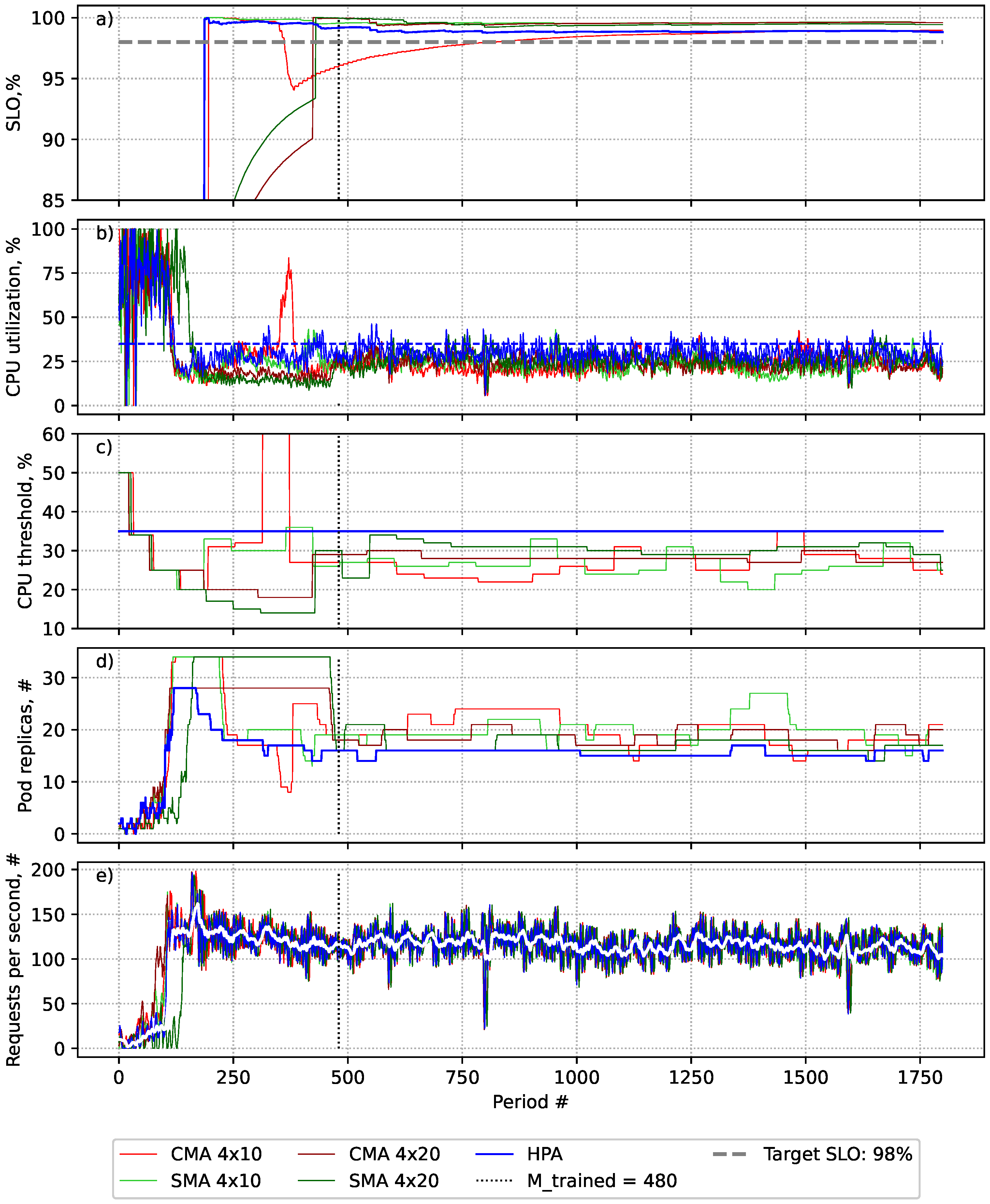
6.3.1. Evaluation of SATA Performance in WorldCup98 Workload Scenario

In this experiment, we assessed the ability of the algorithms to adjust the thresholds under the real-world mixed pattern load. The following settings were applied:

• Load: WorldCup98 on the 78th day from 19:00 to 22:00 and its inverse version.
• Application: calculation of the factorial of a number between 8000 and 12,000.
• Pod replicas: Min: 1, Max: 34.

As the WorldCup98 load in the selected time window had a tendency to increase constantly, its inverse version was appended to see how algorithms perform when the load tends to decrease constantly. The load pattern is presented in Figure 4e.

The experiment results presented in Figure 4 and

Table 5. Results of evaluation of algorithms in WorldCup98 workload scenario.

Approach	CMA 4 × 10	CMA 4 × 20	SMA 4 × 10	SMA 4 × 20	HPA 47%
SLO supported	Fully	Fully	Fully	Fully	Fully
sMAPE, %	1.3	1.4	0.9	1.8	1.4
Total pods	43,364	44,157	43,340	45,531	41,773
Difference from the best result for total pods in %	4	6	4	9	0

show that all of the evaluated approaches were compliant with the SLO throughout the experiment.

As can be seen from Figure 4a,b, there is a noticeable decrease in the SLO value when the CPU threshold exceeds the target utilisation threshold of 47% (dark blue dashed line in Figure 4b).

As seen in Figure 4c, in the event of sudden increases in workload, the algorithms decrease the threshold value, and vice versa. At the same time, all the algorithms tend to approach the target utilisation value, aiming to increase efficiency by adjusting the provisioned resource number to actual resource demand. When the load is decreasing, it suggests higher thresholds than the CMA, thus becoming more efficient in downscale scenarios. However, in upscale scenarios, it is less efficient. This can be observed in the last half of the experiment (Figure 4d) for downscale scenarios and in the first half of the experiment for upscale scenarios.

As can be seen from Table 5, SATA required a slightly higher number of pod replicas in all scenarios compared to the HPA. In general, SATA achieved higher precision in 4 × 10 scenarios and was less precise for 4 × 20 scenarios compared to the HPA. When using the CMA as the smoothing method, the length of the threshold evaluation period did not significantly affect the efficiency and accuracy of SATA. However, when adopting the SMA, a longer period had a positive impact on the precision of SATA.

The experiment with the SMA in a 4 × 10 scenario showed the highest accuracy across SATA algorithms while supporting the defined SLO. The performance of the CMA in a 4 × 10 scenario was similar to that of the HPA but with slight overprovisioning. However, the SMA in a 4 × 10 scenario was more accurate in meeting the desired SLO. This is because SATA with SMA smoothing has higher accuracy in detecting threshold values and is more vulnerable to unexpected load growth when a shorter threshold evaluation period is used. This can be seen in Figure 4a at around the 600th and 1200th metrics’ collection periods (light green line).

The HPA with a static threshold was the most efficient, with precision and accuracy similar to SATA with the CMA with a shorter threshold evaluation period (a 4 × 10 scenario). It must be emphasised that it is hard to achieve such precision in practice without knowing the workload and number of violations per threshold in advance, as was done for this experiment, meaning that the threshold might not be suitable to handle the load changes in the pattern in the future, causing SLO violations. The resource overprovisioning of 4% produced by SATA could be considered as neglectable as it is within the HPA tolerance range of 10% [2] and is expected from SLA-fulfilment-oriented solutions. For example, Prametsi et al.’s [51] experiments show that autoscalers that use a performance-based SLI, such as response time, to ensure compliance with the SLA, require more resources than the HPA, which uses CPU-utilisation-based thresholds.

Interestingly, the HPA enabled by the SATA solution achieved the SLO support goal by solely manipulating the threshold values. It dynamically adapted to the workload to ensure that the desired SLO is achieved consistently. As the experiment shows, the SATA solution is self-adaptive to load changes and automatically updates the thresholds to achieve the desired SLO. The SATA increases the threshold value in the case of downscaling, leading to faster downscaling and resulting cost savings. In the case of a load increase, it automatically decreases the threshold, leading to faster resource provisioning and minimising SLO violations.

The next section describes the experiments with a slightly shaky workload scenario.

6.3.2. Evaluation of SATA Performance in EDGAR Workload Scenario

In this experiment, we assessed the ability of the algorithms to adjust the thresholds under the real-world shaky load pattern. The following settings were applied:

• Load: EDGAR access logs on 30 July 2023, from 02:00 to 05:00.
• Application: calculation of the factorial of a number between 8000 and 12,000.
• Pod replicas: Min: 1, Max: 27.

Figure 5e presents the EDGAR workload. While the load might be seen as constant, it contains a big number of periods where the load changes unexpectedly, but with low magnitude, that is the number of requests changes more than twice in a short period of time, e.g., see the number of events at around 600th the 900th monitoring periods.

The experiment results are presented in Figure 5 and

Table 6. Results of evaluation of algorithms in EDGAR workload scenario.

Approach	CMA 4 × 10	CMA 4 × 20	SMA 4 × 10	SMA 4 × 20	HPA 35%
SLO supported	Partially	Fully	Fully	Fully	Fully
sMAPE, %	0.7	1.6	1.6	1.5	0.9
Total pods	25,329	24,066	25,953	21,955	20,021
Difference from the best result for total pods in %	27	20	29	10	0

. As seen in Figure 5a, all of the evaluated approaches were compliant with the SLO throughout the experiment, with the exception of the SATA CMA 4 × 10 use case, where the suggested threshold value was higher than required. However, the system has been adjusted in the next two upscale periods by altering the thresholds, and hence, the operation has been restored to the desired level. The HPA algorithm was the most accurate in maintaining the target SLO value.

As seen in Figure 5a,b, any increase in CPU utilisation above 35% caused a decrease in the SLO value. As presented in Figure 5c, SATA suggested lower threshold values in all cases as the solution is sensitive to frequent load fluctuations. However, longer threshold evaluation periods resulted in better stability and adjustment of the threshold to a value close to 35%. All scenarios, with the exception of CMA 4 × 10, showed similar accuracy, with SMA 4 × 20 demonstrating slightly better accuracy in identifying the target utilisation threshold. Thus, HPA with SMA 4 × 20 operated closer to the desired utilisation threshold of 35%, resulting in more efficient resource provisioning than other SATA setups, as seen in Figure 5d and Table 6.

During the experiment, it was observed that, in the HPA without the SMA scenario, the supported SLO values began to decrease towards the end of the experiment, as depicted in Figure 5a. This suggests that the current baseline threshold may not be suitable for future workload changes and might not restore the SLO. On the other hand, the SATA approaches have proven to be effective in ensuring compliance with the SLO and the ability to restore the SLO, as evidenced by the achieved results.

As presented in Table 6, the HPA achieved the best resource-management efficiency and accuracy across algorithms that met the SLO during all evaluation periods. The CMA 4 × 10 had the best accuracy, but did not manage to support the SLO in all periods, even though it was the second most overprovisioning solution in this experiment. In Section 6.2, it is shown that, while SMA’s tendency to underestimate the target utilisation threshold improves efficiency in volatile load scenarios, it causes a decrease in efficiency when the load is stable, as evidenced by the data presented in Table 6. According to the results, SMA 4 × 20 performed the best in terms of accuracy and efficiency across all SATA settings and had only 10% overprovisioning in comparison to the HPA with a static threshold setup. As mentioned in Section 6.3.1, overprovisioning is expected, and a 10% overprovisioning rate can be considered a good outcome when the algorithm’s aim is to ensure SLA fulfilment.

The experiments conducted with the WorklCup98 and EDGAR workloads demonstrated that, depending on the workload pattern and SATA settings, the solution can identify thresholds that allow the system to operate close to the defined SLO. The amount of resource overprovisioning can vary from negligible to deviating from 10% to 30% depending on the workload and settings. This is in comparison to using the Horizontal Pod Autoscaler (HPA) with the target utilisation threshold set as closely as possible to the value that allows the system to operate at a performance level where the number of violations does not exceed the maximum allowed. This value is never known upfront, so, in practice, it is challenging to achieve such precision threshold settings. As a result, such a level of overprovisioning is expected.

This section presents the experiments conducted in this work and the achieved results. The next section aims to conclude and discuss the results.

7. Discussion and Conclusions

Container orchestration solutions have become increasingly popular with the rise of containerised applications. The Kubernetes platform is the most widely used container orchestration solution and has its own implementation for horizontal application autoscaling, known as the Horizontal Pod Autoscaler. Determining resource utilisation thresholds for the HPA to ensure desired service levels can be challenging. In an effort to address the limitations of the HPA, various attempts have been made to implement alternative solutions. However, these alternatives would require the implementation of autoscaling solutions that are not natively supported by Kubernetes. Additionally, such alternative solutions have relied on machine learning algorithms [7,12,28] or complex rules [17,27], which may be challenging to understand for those without a deep understanding of the field.

In this work, a threshold-detection approach and SATA prototype for dynamic threshold adjustment were presented. The approach is based on data explanatory analysis and moving average smoothing, which helps to understand and implement the solution without extensive knowledge of machine learning. The SATA prototype, using the Simple Moving Average, is able to detect the desired threshold in real-world workloads with slight overprovisioning. On the other hand, the Centred Moving Average approach showed better accuracy, but was less stable in meeting the SLO values. Therefore, the SMA method is recommended to ensure SLO compliance, and the CMA can be used when cost saving is more important in volatile load scenarios. Longer evaluation periods showed better efficiency where there is a low deviation in the load; in contrast, shorter threshold evaluation periods allowed the algorithm to perform more efficiently in scenarios with high-variation loads.

Interestingly, the experiments revealed that, while the experiments used the same application and pods with the same resource settings, different target utilisation values must be applied depending on the load pattern in order to ensure compliance with the SLO. Based on that, it can be concluded that approaches that use load testing on a single pod instance to determine the maximum CPU utilisation at which the application’s performance meets the SLO requirements may not be sufficient for determining the target utilisation threshold for the HPA.

To improve the algorithm’s performance, it can be customised by adjusting the threshold and evaluation period length based on the expected load pattern. The type of moving average can also be selected to control accuracy depending on the load pattern, whether it is highly volatile or not. Overall, the developed dynamic threshold-detection approach showed good potential. Further prototype stability improvement, experimentation with different SLIs, and adopting the approach to other autoscaling solutions are areas for future research and improvements.

References

1. The Kubernetes Authors. Kubernetes. Available online: https://kubernetes.io/ (accessed on 30 September 2023).
2. Horizontal Pod Autoscaling. Available online: https://kubernetes.io/docs/tasks/run-application/horizontal-pod-autoscale/ (accessed on 30 September 2023).
3. Shafi, N.; Abdullah, M.; Iqbal, W.; Erradi, A.; Bukhari, F. Cdascaler: A cost-effective dynamic autoscaling approach for containerized microservices. In Cluster Computing; Springer: Berlin/Heidelberg, Germany, 2024; pp. 1–21. [Google Scholar] [CrossRef]
4. Best practices for running cost-optimized Kubernetes applications on GKE|Cloud Architecture Center|Google Cloud.
5. Sahal, R.; Khafagy, M.H.; Omara, F.A. A Survey on SLA Management for Cloud Computing and Cloud-Hosted Big Data Analytic Applications. Int. J. Database Theory Appl. 2016, 9, 107–118. [Google Scholar] [CrossRef]
6. Huo, Q.; Li, S.; Xie, Y.; Li, Z. Horizontal Pod Autoscaling based on Kubernetes with Fast Response and Slow Shrinkage. In Proceedings of the 2022 International Conference on Artificial Intelligence, Information Processing and Cloud Computing, AIIPCC 2022, Kunming, China, 19–21 August 2022; pp. 203–206. [Google Scholar] [CrossRef]
7. Khaleq, A.A.; Ra, I. Intelligent Autoscaling of Microservices in the Cloud for Real-Time Applications. IEEE Access 2021, 9, 35464–35476. [Google Scholar] [CrossRef]
8. Rzadca, K.; Findeisen, P.; Swiderski, J.; Zych, P.; Broniek, P.; Kusmierek, J.; Nowak, P.; Strack, B.; Witusowski, P.; Hand, S.; et al. Autopilot: Workload autoscaling at Google. In Proceedings of the 15th European Conference on Computer Systems, EuroSys 2020, Heraklion, Greece, 27–30 April 2020. [Google Scholar] [CrossRef]
9. Al-Haidari, F.; Sqalli, M.; Salah, K. Impact of CPU Utilization Thresholds and Scaling Size on Autoscaling Cloud Resources. In Proceedings of the 2013 IEEE 5th International Conference on Cloud Computing Technology and Science, Bristol, UK, 2–5 December 2013; pp. 256–261. [Google Scholar] [CrossRef]
10. Balla, D.; Simon, C.; Maliosz, M. Adaptive scaling of Kubernetes pods. In Proceedings of the IEEE/IFIP Network Operations and Management Symposium 2020: Management in the Age of Softwarization and Artificial Intelligence, NOMS 2020, Budapest, Hungary, 20–24 April 2020. [Google Scholar] [CrossRef]
11. Makroo, A.; Dahiya, D. A Systematic Approach to Deal with Noisy Neighbour in Cloud Infrastructure. Indian J. Sci. Technol. 2016, 9, 1–9. [Google Scholar] [CrossRef]
12. Kang, P.; Lama, P. Robust resource scaling of containerized microservices with probabilistic machine learning. In Proceedings of the 2020 IEEE/ACM 13th International Conference on Utility and Cloud Computing, UCC 2020, Leicester, UK, 7–10 December 2020; pp. 122–131. [Google Scholar] [CrossRef]
13. DATADOG. 10 Insights on Real-World Container Use|Datadog. Available online: https://www.datadoghq.com/container-report/ (accessed on 10 February 2024).
14. Amiri, M.; Mohammad-Khanli, L. Survey on prediction models of applications for resources provisioning in cloud. J. Netw. Comput. Appl. 2017, 82, 93–113. [Google Scholar] [CrossRef]
15. Dang-Quang, N.M.; Yoo, M.; De, J.F.; Santana, P. Deep Learning-Based Autoscaling Using Bidirectional Long Short-Term Memory for Kubernetes. Appl. Sci. 2021, 11, 3835. [Google Scholar] [CrossRef]
16. Xu, Y.; Qiao, K.; Wang, C.; Zhu, L. LP-HPA: Load Predict-Horizontal Pod Autoscaler for Container Elastic Scaling. In Proceedings of the 5th International Conference on Computer Science and Software Engineering, Guilin, China, 21–23 October 2022; pp. 591–595. [Google Scholar] [CrossRef]
17. Pozdniakova, O.; Cholomskis, A.; Mažeika, D. Self-adaptive autoscaling algorithm for SLA-sensitive applications running on the Kubernetes clusters. In Cluster Computing; Springer: Berlin/Heidelberg, Germany, 2023; pp. 1–28. [Google Scholar] [CrossRef]
18. Wu, Q.; Yu, J.; Lu, L.; Qian, S.; Xue, G. Dynamically adjusting scale of a Kubernetes cluster under QoS guarantee. In Proceedings of the International Conference on Parallel and Distributed Systems—ICPADS, Tianjin, China, 4–6 December 2019; pp. 193–200. [Google Scholar] [CrossRef]
19. Likosar, B. Getting the Most from Kubernetes Autoscaling—The New Stack, 2023. Available online: https://thenewstack.io/getting-the-most-from-kubernetes-autoscaling/ (accessed on 10 February 2024).
20. Nguyen, T.T.; Yeom, Y.J.; Kim, T.; Park, D.H.; Kim, S. Horizontal pod autoscaling in Kubernetes for elastic container orchestration. Sensors 2020, 20, 4621. [Google Scholar] [CrossRef] [PubMed]
21. Augustyn, D.R.; Wyci´slik, L.W.; Sojka, M. Tuning a Kubernetes Horizontal Pod Autoscaler for Meeting Performance and Load Demands in Cloud Deployments. Appl. Sci. 2024, 14, 646. [Google Scholar] [CrossRef]
22. Huo, Q.; Li, C.; Li, S.; Xie, Y.; Li, Z. High Concurrency Response Strategy based on Kubernetes Horizontal Pod Autoscaler. J. Phys. Conf. Ser. 2023, 2451, 012001. [Google Scholar] [CrossRef]
23. Baresi, L.; Hu, D.Y.X.; Quattrocchi, G.; Terracciano, L. KOSMOS: Vertical and Horizontal Resource Autoscaling for Kubernetes. In Service-Oriented Computing. ICSOC 2021; Lecture Notes in Computer Science; Springer: Cham, Switzerland, 2021; Volume 13121, pp. 821–829. [Google Scholar] [CrossRef]
24. Phuc, L.H.; Phan, L.A.; Kim, T. Traffic-Aware Horizontal Pod Autoscaler in Kubernetes-Based Edge Computing Infrastructure. IEEE Access 2022, 10, 18966–18977. [Google Scholar] [CrossRef]
25. Cao, Y.; Maghsudi, S.; Ohtsuki, T. Mobility-Aware Routing and Caching: A Federated Learning Assisted Approach. In Proceedings of the ICC 2021—IEEE International Conference on Communications, Montreal, QC, Canada, 14–23 June 2021. [Google Scholar] [CrossRef]
26. Ruiz, L.M.; Pueyo, P.P.; Mateo-Fornes, J.; Mayoral, J.V.; Tehas, F.S. Autoscaling Pods on an On-Premise Kubernetes Infrastructure QoS-Aware. IEEE Access 2022, 10, 33083–33094. [Google Scholar] [CrossRef]
27. Beloglazov, A.; Buyya, R. Adaptive threshold-based approach for energy-efficient consolidation of virtual machines in cloud data centers. In Proceedings of the 8th International Workshop on Middleware for Grids, Clouds and e-Science, New York, NY, USA, 29 November–3 December 2010; pp. 1–6. [Google Scholar] [CrossRef]
28. Horovitz, S.; Arian, Y. Efficient Cloud Auto-Scaling with SLA Objective Using Q-Learning. In Proceedings of the 2018 IEEE 6th International Conference on Future Internet of Things and Cloud, FiCloud 2018, Barcelona, Spain, 6–8 August 2018; pp. 85–92. [Google Scholar] [CrossRef]
29. Taherizadeh, S.; Stankovski, V. Dynamic Multi-level Auto-scaling Rules for Containerized Applications. Comput. J. 2019, 62, 174–197. [Google Scholar] [CrossRef]
30. Tran, M.N.; Vu, D.D.; Kim, Y. A Survey of Autoscaling in Kubernetes. In Proceedings of the International Conference on Ubiquitous and Future Networks, ICUFN, Barcelona, Spain, 5–8 July 2022; pp. 263–265. [Google Scholar] [CrossRef]
31. Qu, C.; Calheiros, R.N.; Buyya, R. Auto-scaling web applications in clouds: A taxonomy and survey. ACM Comput. Surv. 2018, 51, 33. [Google Scholar] [CrossRef]
32. Lord, D.; Qin, X.; Geedipally, S.R. Exploratory analyses of safety data. In Highway Safety Analytics and Modeling; Elsevier: Amsterdam, The Netherlands, 2021; pp. 135–177. [Google Scholar] [CrossRef]
33. Han, J.; Kamber, M.; Pei, J. Getting to Know Your Data. In Data Mining; Cambridge University Press: Cambridge, UK, 2012; pp. 39–82. [Google Scholar] [CrossRef]
34. Dash, C.S.K.; Behera, A.K.; Dehuri, S.; Ghosh, A. An outliers detection and elimination framework in classification task of data mining. Decis. Anal. J. 2023, 6, 100164. [Google Scholar] [CrossRef]
35. Sidekerskiene, T.; Damasevicius, R. Reconstruction of Missing Data in Synthetic Time Series Using EMD. In Proceedings of the International Conference for Young Researchers in Informatics, Mathematics and Engineering, Catania, Italy, 27–29 June 2016; Volume 1712, pp. 7–17. [Google Scholar]
36. Raudys, A.; Lenčiauskas, V.; Malčius, E. Moving averages for financial data smoothing. Commun. Comput. Inf. Sci. 2013, 403, 34–45. [Google Scholar] [CrossRef]
37. Hyndman, R.J.; Athanasopoulos, G. Forecasting: Principles and Practice, 2nd ed.; Melbourne, Australia, 2018; Available online: https://otexts.com/fpp2/ (accessed on 30 January 2024).
38. Hyndman, R.J. Rob J Hyndman—Thoughts on the Ljung-Box Test, 2014. Available online: https://robjhyndman.com/hyndsight/ljung-box-test/ (accessed on 30 January 2024).
39. Microsoft. Azure Kubernetes Service (AKS) Documentation. Available online: https://learn.microsoft.com/en-us/azure/aks/ (accessed on 10 February 2024).
40. Gatling—Professional Load Testing Tool. Available online: https://gatling.io/ (accessed on 10 February 2024).
41. Microsoft. Load Balancer. Available online: https://learn.microsoft.com/en-us/azure/load-balancer/ (accessed on 30 September 2023).
42. olesiapoz/sata: The SLA-Adaptive Threshold Adjustment Algorithm for Kubernetes Horizontal Autoscaler. Available online: https://github.com/olesiapoz/sata (accessed on 30 January 2024).
43. Prometheus—Monitoring System & Time Series Database. Available online: https://prometheus.io/ (accessed on 30 January 2024).
44. Chen, C.; Twycross, J.; Garibaldi, J.M. A new accuracy measure based on bounded relative error for time series forecasting. PLoS ONE 2017, 12, e0174202. [Google Scholar] [CrossRef]
45. 1998 World Cup Web Site Access Logs. Available online: https://zenodo.org/records/5145855 (accessed on 10 February 2024).
46. SEC.gov|EDGAR Log File Data Sets. Available online: https://www.sec.gov/about/data/edgar-log-file-data-sets (accessed on 30 January 2024).
47. Bogachev, M.I.; Kuzmenko, A.V.; Markelov, O.A.; Pyko, N.S.; Pyko, S.A. Approximate waiting times for queuing systems with variable long-term correlated arrival rates. Phys. A Stat. Mech. Its Appl. 2023, 614, 128513. [Google Scholar] [CrossRef]
48. Imdoukh, M.; Ahmad, I.; Alfailakawi, M.G. Machine learning-based auto-scaling for containerized applications. Neural Comput. Appl. 2020, 32, 9745–9760. [Google Scholar] [CrossRef]
49. Ye, T.; Guangtao, X.; Shiyou, Q.; Minglu, L. An Auto-Scaling Framework for Containerized Elastic Applications. In Proceedings of the 2017 3rd International Conference on Big Data Computing and Communications, BigCom 2017, Chengdu, China, 10–11 August 2017; pp. 422–430. [Google Scholar] [CrossRef]
50. Markfjärd, G. SLA-Aware Microservice Orches-Tration-Investigating How to Include SLA Resilience When Updating and Scaling Microservices. Ph.D. Thesis, Linköping University, Linköpings, Sweden, 2021. [Google Scholar]
51. Pramesti, A.A.; Kistijantoro, A.I. Autoscaling Based on Response Time Prediction for Microservice Application in Kubernetes. In Proceedings of the 2022 9th International Conference on Advanced Informatics: Concepts, Theory and Applications, ICAICTA 2022, Tokoname, Japan, 28–29 September 2022. [Google Scholar] [CrossRef]
Figure 1. (a) A line graph of the achieved Service Levele Objective (SLO) values per CPU range without smoothing. (b) A line graph of the achieved Service Levele SLO values per CPU range using Simple Moving Average smoothing. (c) A line graph of the achieved SLO values per CPU range using Centred Moving Average smoothing. Dots represent the SLO achieved in the experiments when the Horizontal Pod Autoscaler (HPA) was configured with a static CPU utilisation threshold.
Electronics 13 01242 g001
Figure 2. Evaluation of the impact of threshold adjustment and evaluation period length on the effectiveness of the SLA-adaptive threshold adjustment (SATA) solution using Simple Moving Average (SMA). (a) The SLO value after collecting a sufficient number of events (after the dotted line). (b) The average CPU utilisation. (c) The applied target utilisation threshold in each period. (d) The number of pods provisioned in each period. (e) The generated workload requests per second.
Electronics 13 01242 g002
Figure 3. Evaluation of adoption of Centred Moving Average and Simple Moving Average on SLA-adaptive threshold adjustment (SATA) solution performance in On–off workload scenario. (a) The achieved SLO value after collecting a sufficient number of events. (b) The average CPU utilisation. (c) The applied target utilisation threshold at each period. (d) The number of pods provisioned in each period. (e) The generated workload requests per second.
Electronics 13 01242 g003
Figure 4. An evaluation of the SLA-adaptive threshold adjustment (SATA) solution using two different smoothing techniques—Simple Moving Average (SMA) and Centred Moving Average (CMA)—with two different settings: T a d j u s t = 4 and T e v a l = 10 autoscaling periods (4 × 10) and T a d j u s t = 4 and T e v a l = 20 autoscaling periods (4 × 20) for the WorldCup98 workload scenario. (a) The achieved SLO value after collecting a sufficient number of events. (b) Average CPU utilisation. (c) The number of pods provisioned in each period. (d) The applied target utilisation threshold in each period. (e) The generated workload requests per second.
Electronics 13 01242 g004
Figure 5. An evaluation of the SLA-adaptive threshold adjustment (SATA) solution using two different smoothing techniques—Simple Moving Average (SMA) and Centred Moving Average (CMA)—with two different settings: T a d j u s t = 4 and T e v a l = 10 autoscaling periods (4 × 10) and T a d j u s t = 4 and T e v a l = 20 autoscaling periods (4 × 20) for the EDGAR workload scenario. (a) The achieved SLO value after collecting a sufficient number of events. (b) Average CPU utilisation. (c) The number of pods provisioned in each period. (d) The applied target utilisation threshold in each period. (e) The generated workload requests per second.
Electronics 13 01242 g005