A Method of Diagnosing Analog Circuit Soft Faults Using Boruta Features and LightGBM

Abstract

Modern electronic power systems rely heavily on analog circuits. The accurate detection of analog circuit faults, especially soft faults, is of great significance for the maintenance and inspection of electronic systems. This paper proposes the application of the Boruta feature selection method to the field of the soft fault diagnosis of analog circuits to screen out low-dimensional and efficient feature components from the high-dimensional time-domain statistical features and frequency-domain features of circuit responses. Then, the feature components are used as the input to train the LightGBM classification model, and the Bayesian optimization method is introduced to optimize the model’s hyperparameters. Finally, the trained fault diagnosis model is verified in two typical experimental circuits, and satisfactory accuracy is obtained.

1. Introduction

The electronic circuit industry’s rapid evolution has propelled sophisticated devices into nearly every aspect of our lives, from industrial production to everyday conveniences. As these circuits become increasingly integrated, their functionalities and modularity are also growing, demanding heightened operational reliability. This imperative is particularly critical in demanding fields like aerospace, military, and medicine, where systems often operate under extreme conditions [1]. Achieving stable, error-free performance is paramount in these applications. Failure to diagnose faults promptly can lead to significant consequences.

While electronic circuits come in two flavors—digital and analog—troubleshooting issues in the latter proves significantly more demanding. This stems from several inherent characteristics of analog circuits: component complexities, measurement uncertainties, limited observability, etc. Despite these challenges, the significance of analog circuits cannot be understated. Even in mixed-signal devices where digital circuits dominate in number, 80% of faults occur in the analog portions [2]. This highlights the critical need for advancements in analog fault diagnosis techniques.

Two distinct categories encompass the fault diagnosis methods applicable to analog circuits which are called model-based and data-driven methods. The former generally hopes to derive the transfer function equation of the circuit, mainly through analyzing the circuit design principle or adopting some parameter identification techniques. Obviously, for simple circuits, such methods usually have certain effects. Nevertheless, with the escalating complexity of the circuit, the difficulty of obtaining a usable transfer function equation, or even just estimating some parameters, is greatly increased, and it is quite challenging. Relatively speaking, data-driven methods are more popular and have more operability.

There exist two distinct categories of faults in analog circuits. The first type is called a hard fault, which refers to the open circuit or short circuit caused by the physical damage or connection error of electronic components. In serious cases, it can lead to the circuit being completely unable to work. Many people have done relevant research on the open-circuit and short-circuit phenomena of some special circuits. Wang et al. [3] combined an improved Dempster–Shafer (DS) evidence theory with a backpropagation (BP) neural network to enhance the accuracy of diagnosing open-circuit faults in inverter transistors. Mingyun Chen et al. [4] developed a fault injection strategy to aid in differentiating between internal and external switch faults within 3L-NPC rectifiers. Their method facilitates the quick and accurate detection of both single and multiple switch faults, improving overall system reliability. Tiancheng Shi [5] introduced an enhanced diagnostic approach utilizing a deep belief network (DBN) in conjunction with the least squares support vector machine (LSSVM). This method proves highly effective in diagnosing diverse switch faults within pulse-width modulation voltage source rectifier systems, showcasing a robust resistance to interference and swift fault identification.

Another type is called a soft fault. Soft faults in analog circuits refer to instances where component parameters deviate from expectations due to external factors such as temperature variations, electromagnetic interference, prolonged usage, etc. These deviations can render the circuit inoperable under certain conditions. In contrast to most hard faults, soft faults exhibit a more covert nature and pose greater challenges for detection [6]. Scholars have extensively explored data-driven approaches to address soft fault issues in electronic circuits, recognizing the need for advancements in this field. Mehran Aminian and Farzan Aminian [7] have successively attempted to employ the PCA [8] method to reduce the dimensionality of features obtained through wavelet transformation. Yingqun Xiao et al. [9] have introduced a distinctive preprocessing technique, referred to as kernel principal components analysis with a focus on maximal class separability, for analyzing the time response of the analog circuit. Lipeng Ji et al. [10] leveraged the formidable of ResNet networks in feature extraction and learning to identify crucial parameters defining analog circuit performance to pinpoint the failing component. Ping Song et al. [11] introduced a novel approach for fault feature extraction utilizing fractional Fourier transform (FRFT), and SVM was employed to train the extracted features to achieve the effect of diagnosing and categorizing the faults. Peng Sun et al. [12] introduced a fault diagnosis method for modular analog circuits, utilizing support vector data description (SVDD) and integrating Dempster–Shafer (abbreviated as DS) evidence theory. They performed simulation and hardware experiments on a double-bandpass filter circuit, achieving favorable results. Chaolong Zhan [13] introduced deep belief networks into the fault diagnosis of analog circuits, and used a particle swarm optimization algorithm (QPSO) to optimize the learning rate of a DBN. Huahui Yang et al. [14] applied convolutional neural networks in one dimension for diagnosing faults in analog circuits, aiming to simultaneously complete the tasks of extracting relevant features and classifying faults within the input signal through the neural network. Zhijie Yuan [15] used two popular methods in manifold learning methods, local linear embedding (LLE) and diffusion mapping (DM), to optimize the dimensionality reduction techniques commonly used, so as to better extract the fault features in analog circuits.

From the existing research, it can be seen that most studies follow the practice of first extracting features from circuit signals, then reducing the dimensionality of the features, and finally classifying faults. In the feature extraction step, many time-domain statistical features are often ignored, while these features should be combined with frequency-domain features to more completely represent the fault features of the circuit. However, this combination will increase the dimension of the feature vector, and it is necessary to exclude some less correlated and redundant feature parts from these high-dimensional features to reduce the pressure of subsequent fault classification. To that aim, this paper introduces a novel approach to diagnose faults in analog circuits, which relies on Boruta feature selection and the LightGBM model. In order to achieve this, we rely on the technical contributions listed below:

(i)

We use several time-domain statistical feature methods to extract the statistical features of the time-domain signal and use wavelet packet transform to extract the frequency features of the time-domain signal. By combining the two, the composite feature vector of the circuit signal is obtained.

(ii)

The Boruta feature selection method is proposed to extract low-dimensional effective features from high-dimensional feature vectors.

(iii)

The LightGBM model is proposed as a means for diagnosing analog circuit faults. We also introduce the Bayesian optimization approach to effectively fine-tune the hyperparameters of the model for enhanced performance.

The subsequent sections are structured as follows: Section 2 presents the pertinent theoretical framework utilized in this research. Section 3 elaborates on the procedural steps of the proposed methodology. In Section 4, the application of the proposed method to two experimental circuits is discussed, along with an analysis of the experimental findings. Additionally, a comparative experiment is outlined to showcase the efficacy of the proposed approach. Finally, Section 5 provides a summary of the research conducted in this paper.

2. Related Theories

2.1. Boruta Feature Selection

The Boruta feature selection technique is categorized as a wrapper-based approach for feature selection. Unlike filter-based methodologies, wrapper-based techniques evaluate the significance of features by analyzing their performance within predictive models. They aim to identify the most suitable subset of features while ensuring robustness against irrelevant or noisy features [16]. Boruta is an all-relevant feature selection method, while most other methods are minimally optimal. This means that it aims to find all the features that carry information for prediction, rather than finding a possible compact subset of features in which some classifiers have the minimum error amount. The detailed algorithm steps are as follows [17]:

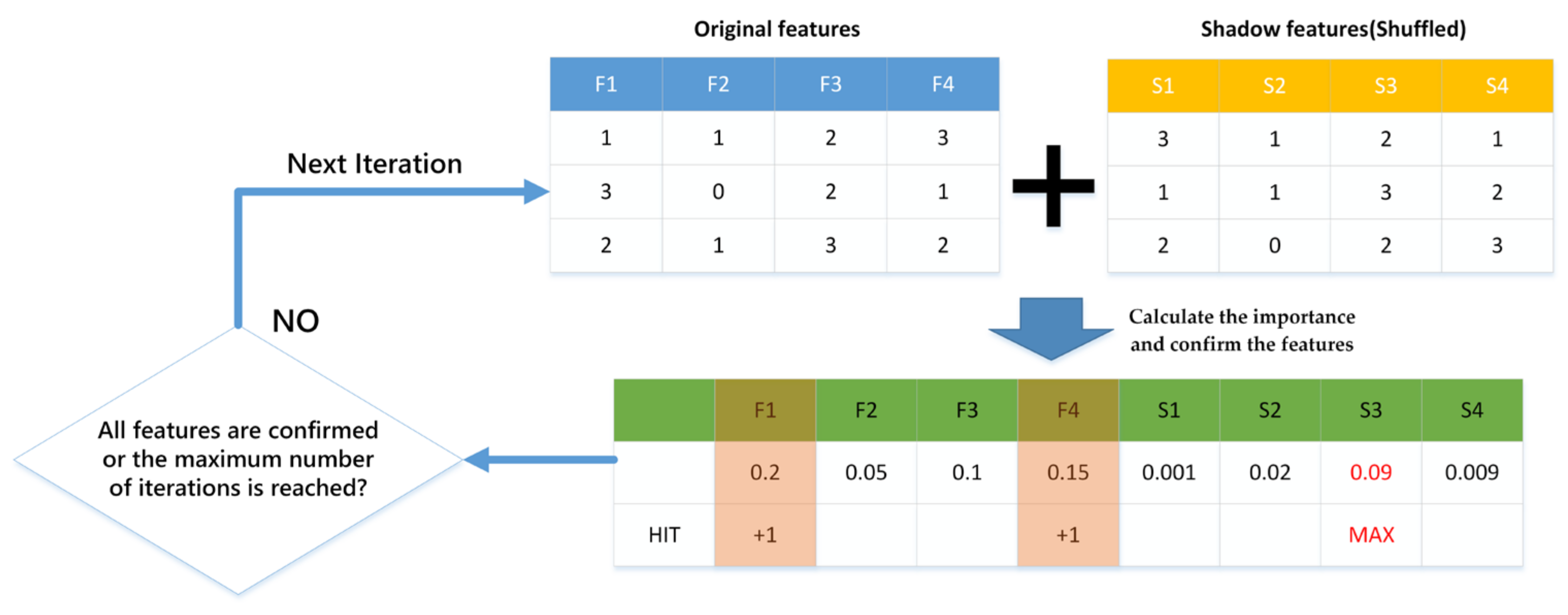
Step 1: Initialization. First, randomly generate a shadow dataset, where the values of each feature are the shuffled values of that feature in the original dataset. Then, combine the original dataset and the shadow dataset to obtain an extended dataset.

Step 2: Train the model. Train a classification model on the extended dataset. In this paper, the LightGBM model is selected. Calculate the importance of each feature, which is represented by the $Z_{score}$ in the following fomula:

$$Z_{score}=\frac{E_f}{f}$$

(1)

where $E_f$ represented the mean of accuracy loss, and $f$ represented the standard deviation of accuracy loss.

Step 3: Confirm the features. Verify each feature to determine if it holds a greater significance than the highest value of the importance score within the shadow feature. If so, confirm the feature as a relevant feature.

Step 4: Iterate. Repeat Step 2 and 3 until all features are confirmed or the set maximum number of iterations is reached.

The above Boruta feature selection method can represented by Figure 1:

2.2. Light Gradient-Boosting Machine (LightGBM)

The light gradient-boosting machine is a gradient-boosting tree model introduced by Microsoft Research Asia in 2016. The origins of the LightGBM can be traced back to the 1990s, a period when gradient-boosting tree models started to garner interest among researchers. Gradient-boosting tree models are an iterative learning approach, progressively enhancing the model’s performance by incorporating a tree during each iteration.

The LightGBM represents a refinement of the gradient-boosting decision tree (GBDT) algorithm, employing weak classifiers such as decision trees to progressively refine the model. Notably, the LightGBM offers advantages in terms of effective training outcomes and a reduced risk of overfitting. In contrast to the GBDT, which necessitates multiple passes through the entire training dataset during each iteration, the LightGBM mitigates the need for loading the complete dataset into memory. This circumvents the limitations on training data size imposed by memory constraints. Moreover, the LightGBM’s approach addresses the time-consuming nature of repeatedly reading and writing training data by implementing specific strategies to optimize performance. The specific implementation methods include the following points [18,19]:

• Histogram-based algorithm. This algorithm addresses eigenvalue segmentation with both memory and computational efficiency. By discretizing continuous eigenvalues into k integers and constructing a corresponding histogram, it avoids extensive data processing. Traversing the data once populates the histogram with relevant statistics, enabling an efficient search for the optimal segmentation point within the discrete representation. This significantly reduces both the memory footprint and the computational complexity compared to alternative methods.
• Leaf-wise growth. Unlike traditional level-wise tree growth, the LightGBM grows trees leaf-wise. Instead of expanding all nodes at a given level, it continuously seeks the leaf with the biggest potential improvement (split gain), leading to a potentially lower error and higher accuracy at the same number of splits.
• Gradient-based one-side sampling (GOSS). GOSS is a smart technique that speeds up learning in decision trees by focusing on informative samples. The key idea of GOSS is that samples with larger gradients (essentially, larger prediction errors) contribute more to information gain. GOSS ranks all samples based on their absolute gradient values, prioritizing those with large errors. To maintain data diversity, the algorithm randomly samples a smaller number of remaining (lower gradient) samples. Then, it adjusts the weights of these randomly selected samples slightly to emphasize their importance without significantly altering the dataset’s overall distribution.
• Exclusive feature bundling (EFB). High dimensional data tend to be sparse, and this sparsity inspires us to design a lossless method to reduce the dimensions of features. Usually, the features that are bundled are mutually exclusive (i.e., they do not have both nonzero values, like one-hot), so that two features are bundled without losing information. If the two features are not mutually exclusive (in some cases, they are both non-zero), we can use a metric called the collision ratio to measure the extent to which the features are not mutually exclusive, and when this value is small, we can choose to combine the two features without affecting the final accuracy. Exclusive feature bundling (EFB) points out that the number of features can be reduced if some features are fused and bound together. This will help to reduce the time complexity when building the histogram.

2.3. Bayesian Optimization

Bayesian optimization is a global optimization technique that leverages Bayesian statistical theory to efficiently search for global optima. In contrast to traditional optimization methods, Bayesian optimization for parameter tuning uses Gaussian processes, taking into account previous parameter information, continually updating prior information, effectively reducing the number of iterations in the tuning process, and demonstrating robust performance when dealing with non-convex problems.

The Bayesian optimization framework primarily comprises two fundamental components: a probabilistic surrogate model and an acquisition function [20]. The probabilistic surrogate model contains a prior probability model and an observation model. In a narrow sense, Bayesian optimization refers to sequential model-based optimization (SMBO) in which the surrogate model is a Gaussian process regression model. Gaussian process regression involves using a Gaussian process model $F\left(x\right)$ to the target function $f\left(x\right)$. Initially, the predefined mean function $m\left(x\right)$ and covariance function $K\left(x,x\prime \right)$ are established as the prior distribution of the Gaussian process. Next, the sampling indices $x_1,x_2,\dots ,x_t$ are selected, obtaining observed values of the target function $f\left(x_1\right),\dots ,f\left(x_t\right)$, which correspondingly are the random variables $F\left(x_1\right),\dots ,F\left(x_t\right)$ in the Gaussian process. The parameters of the mean and covariance functions are adjusted based on the observed values, thereby determining the final form of the Gaussian process, completing the fitting of the function $f\left(x\right)$.

Another important part of Bayesian optimization is the acquisition function []. Since the surrogate model outputs the posterior distribution of function $f$, we can utilize this posterior distribution $F\left(x\right)|F\left(x_{1:t}\right)=f\left(x_{1:t}\right)$ to evaluate where the next sampling point should be located. The acquisition function takes the form of $A(x,F\left(x\right)|F\left(x_{1:t}\right)=f\left(x_{1:t}\right))$, where its input scores each sampling point ‘x’, with higher scores indicating points more deserving of being sampled.

Generally, the acquisition function needs to satisfy several criteria. Firstly, it should have smaller values at existing sampling points, as these points have already been explored. Secondly, it should have larger values at points with wider confidence intervals (higher variance) because these points possess greater uncertainty and are more worthy of exploration. For maximization (or minimization) problems, the acquisition function should have larger values at points with higher (or lower) function means, as the mean provides an estimate of the function value at that point, making these points more likely to be near extreme points. There are various choices of acquisition functions. Those commonly used are the probability improvement (PI), expected improvement (EI), and the upper confidence bound (UCB).

In summary, Bayesian optimization is an iterative process that primarily involves three steps:

Step 1: Select the next most promising evaluation point $x_t$ based on maximizing the acquisition function.

Step 2: Evaluate the objective function $y_t=f\left(x_t\right)+{\epsilon }_t$ at the chosen evaluation point $x_t$.

Step 3: Add the newly obtained input-observation pair $\left\{x_t,y_t\right\}$ to the historical observation set $D_{1:t-1}$, and update the probabilistic surrogate model in preparation for the next iteration.

3. Proposed Method

3.1. Obtain the Feature Vector

The time-domain statistical characteristics of a circuit signal provide essential insights into the behavior and properties of the signal. Understanding these features is crucial signal processing, system identification, and fault diagnosis in circuits.

This article selects six typical time-domain statistical features for a set of time-domain signal vectors $X=\left[x_1,x_2,\dots ,x_n\right]$, including the standard deviation, kurtosis, skewness, entropy, waveform factor and impulse indicator:

Standard deviation is used to measure the dispersion of the data, with a larger standard deviation indicating greater data spread, and is defined as Equation (2):

$$\sigma =\sqrt{\frac{1}{N}{\displaystyle \sum _{n=1}^N{(x_n-\mu )}^2}}$$

(2)

Kurtosis is used to describes the steepness of the data distribution, where a higher kurtosis indicates relatively concentrated data and a lower kurtosis indicates a flatter distribution. It is defined as follows.

$$KU=\frac{\frac{1}{N}{\displaystyle {\sum }_{n=1}^N{(x_n-\mu )}^4}}{{\sigma }^4}-3$$

(3)

Skewness is used to measures the asymmetry of the data distribution, with positive skewness indicating right-skewed data and negative skewness indicating left-skewed data, and is defined as follows.

$$SK=\frac{\frac{1}{N}{\displaystyle {\sum }_{n=1}^N{(x_n-\mu )}^3}}{{\sigma }^3}$$

(4)

Entropy is used to measure the complexity or uncertainty of a signal, where higher entropy values indicate greater signal complexity or uncertainty. Entropy is defined as follows.

$$e=-{\displaystyle \sum _{i}P(x=a_i)\log P(x=a_i)}$$

(5)

The waveform factor is defined as follows. It is used to described the degree of distortion of a signal waveform.

$$SH(X)=\frac{RMS(X)}{\frac{1}{N}{\displaystyle {\sum }_{n=1}^N\left|x_n\right|}}$$

(6)

where RMS represents for root mean square.

The impulse indicator is used to described the impulsive characteristics of a signal and is defined as follows.

$$IM(X)=\frac{\max \left|X\right|}{\frac{1}{N}{\displaystyle {\sum }_{n=1}^N\left|x_n\right|}}$$

(7)

In addition to time-domain statistical features, we also selected wavelet packet transform (WPT), a representative signal frequency-domain feature extraction method [21,22], to extract the frequency-domain features of analog circuit responses. WPT is a further decomposition of high-frequency signals on the basis of wavelet transform. The general process is as shown in Figure 2. After n layers of decomposition, the original signal can be decomposed into 2ⁿ sub-bands.

Assume that the initial signal is given by $d_0^1=f\left(n\right)$, which could be represented after WPT as follows:

$$d_l^{j,2n}={\displaystyle \sum _k{h}_{k-2l}{d}_k^{j+1,n}}$$

(8)

$$d_l^{j,2n+1}={\displaystyle \sum _k{g}_{k-2l}{d}_k^{j+1,n}}$$

(9)

where $d_l^{j,2n}$ and $d_l^{j,2n+1}$ refer to the node coefficients of node $\left(j,n\right)$ in the layer $l$ of the wavelet packet decomposition under a high-pass filter and low-pass filter, respectively. $h_{k-2l}$ and $g_{k-2l}$ refer to the high-pass and low-pass filters. $d_k^{j+1,n}\left(n\right)$ is the node coefficient of node $\left(j+1,n\right)$ at layer k of the wavelet packet.

The energy of the kth layer and jth band is defined as follows:

$$E_k^j={\displaystyle \sum _{n=1}^M|d_k^{j,n}{|}^2,j=0,1,2,\dots ,2^k-1}$$

(10)

where M denotes the length of the jth band.

And the corresponding band spectrum coefficient is:

$$r_j=\frac{E_j}{E},j=0,1,2,\dots ,2^k-1$$

(11)

where E denotes the total energy of the kth layer. Thus, the sequence $\left\{r_j,j=0,1,2,\dots ,2^k-1\right\}$ could be used as the frequency-domain feature of the signal.

In this paper, we combine the 6-dimensional statistical features of circuit responses with the 8-dimensional frequency features extracted by the wavelet packet transform to form a 14-dimensional feature vector. Then, we use the Boruta method to perform a feature screening on the 14-dimensional features to achieve a feature dimension reduction. After that, we use the reduced features as the input to train the LightGBM model, and optimize the model parameters with the Bayesian optimization method. Finally, we use the model to realize the fault diagnosis of the simulated circuits.

3.2. Steps of the Proposed Method

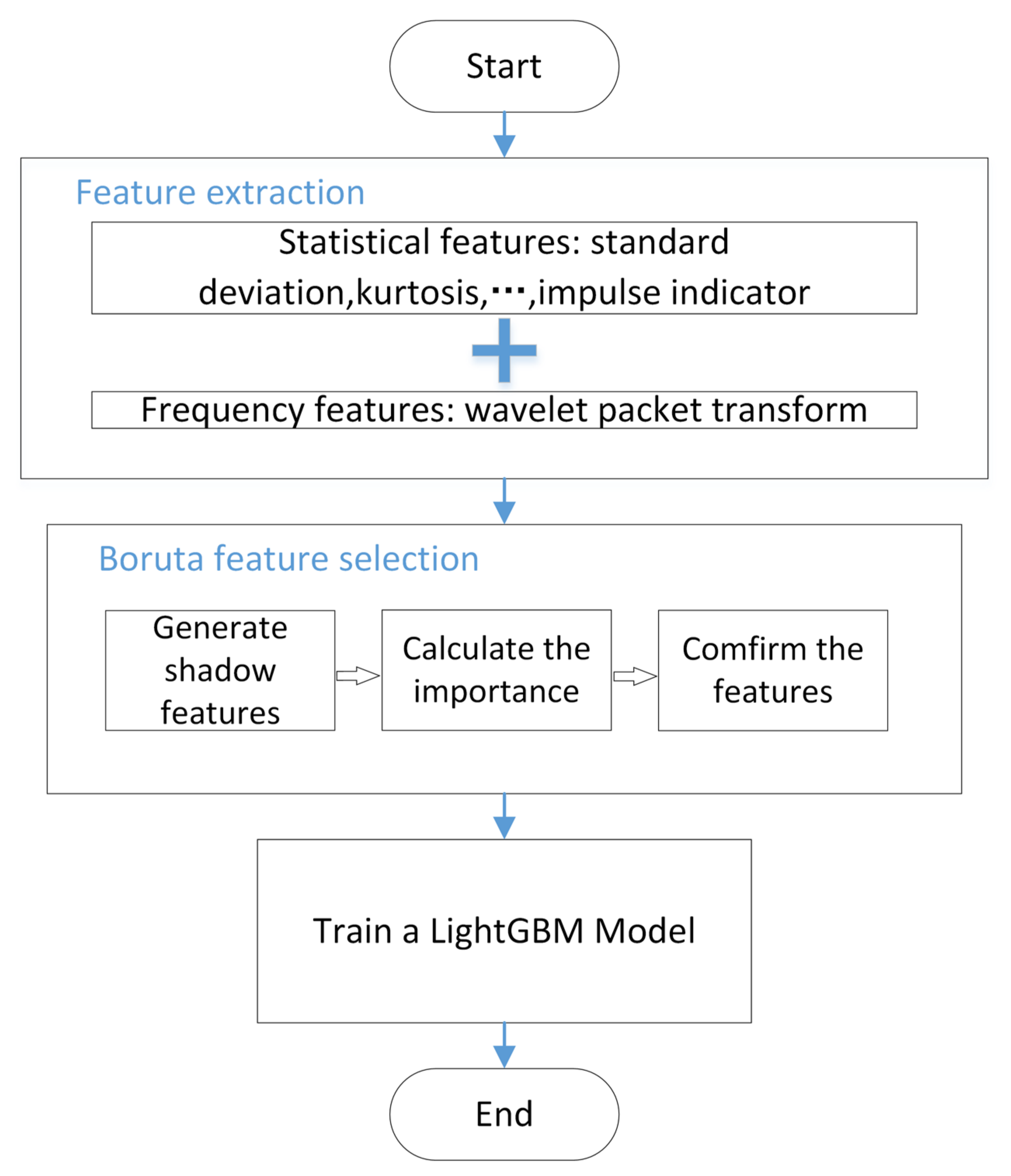
In this section, we outline the fundamental procedures for conducting feature extraction as follows and depicted in Figure 3:

Step 1: Obtain circuit response signals under various fault modes from the experiment circuit. The features of the signals are extracted to obtain high-dimensional feature vectors that simultaneously contain the time-domain statistical features and frequency-domain features of the signals.

Step 2: The Boruta feature selection algorithm is utilized on feature vectors with a high dimensionality to eliminate features that are weakly correlated or redundant.

Step 3: The refined characteristics are utilized as the input for the training of a LightGBM model. Bayesian optimization is utilized to optimize the hyperparameters of the LightGBM model with the aim of improving its classification performance.

4. Analog Circuit Experiment

In this segment, we implemented the suggested approach on two standard circuits to assess its efficacy and dependability. The circuits under consideration are the Sallen–Key band-pass filter circuit and the four opamp biquad high-pass filter circuit. Based on practical experience, circuits rarely have two or more components failing simultaneously; therefore, this paper only considers single fault scenarios.

4.1. Sallen–Key Band-Pass Filter

The initial experimental circuit implemented is the Sallen–Key band-pass filter, as shown in Figure 4. Sallen–Key band-pass filter. This filter configuration comprises five resistors, two capacitors, and a fundamental operational amplifier. Through a sensitivity analysis of the circuit, it is observed that the component values of C1, C2, R2, and R3 play a crucial role in determining the output characteristics of the circuit. Therefore, these components are chosen as potential faulty components. In this paper, component faults are defined as follows: if the actual parameters of a component deviate by 50% or more from its nominal value, the component is considered faulty. The nominal values of the potential faulty components and their fault modes for the Sallen–Key band-pass filter are shown in

Table 1. Nominal and fault values for a Sallen–Key band-pass filter.

Fault Tag	Fault Class	Nominal Value	Fault Value
F0	\	\	\
F1	C1 ↓	5 nF	2.5 nF
F2	C1 ↑	5 nF	7.5 nF
F3	R3 ↑	2 kΩ	3 kΩ
F4	R3 ↓	2 kΩ	1 kΩ
F5	C2 ↓	5 nF	2.5 nF
F6	C2 ↑	5 nF	7.5 nF
F7	R2 ↑	3 kΩ	4.5 kΩ
F8	R2 ↓	3 kΩ	1.5 kΩ

. The symbols “↑” and “↓” in the table indicate that the actual value of the component in this fault type exceeds or falls below its nominal value.

In the circuit simulation setting, according to practical experience, all resistors are set to a 5% tolerance and all capacitors are set to a 10% tolerance. The circuit’s excitation source is an alternating voltage signal with an amplitude of 5 V and a frequency of 1 kHz. The circuit’s sampling time is 1.2 ms. A Monte Carlo analysis is performed on the circuit 100 times under each fault mode, and the circuit’s time-domain output response is extracted.

According to the previous text, the proposed method was used to perform feature selection on the data features using the Boruta method and the selected results are the kurtosis, skewness, and the eighth component of the wavelet packet decomposition. The visualization of the fault features is shown in Figure 5. It can be seen from the figure that the fault features have a good degree of discrimination.

Then, the filtered features were used as input to train a LightGBM model. Bayesian optimization was employed to optimize the model’s hyperparameters. The optimized hyperparameters are shown in

Table 2. Bayesian optimization results of Sallen–Key band-pass filter.

Parameter	Value
n_estimators	296
learning_rate	0.1794
min_child_samples	26
min_child_weight	0.009
min_split_gain	0.89
num_leaves	43

. The classification results of the model on the data are represented by a confusion matrix, as shown in Figure 6. The accuracy of the diagnosis of each type of fault is above 94%, and the overall accuracy reaches 97.8%.

4.2. Four Opamp Biquad High-Pass Filter

The subsequent experimental setup is the four opamp biquad high-pass filter, depicted in Figure 7. This filter comprises ten resistors, two capacitors, and four fundamental operational amplifiers. Through sensitivity analysis, it is observed that the values of R1, R2, R3, R4, C1, and C2 play a crucial role in determining the output characteristics of the circuit. Therefore, these components are chosen as potential faulty components. Similarly, if the actual parameters of an electronic component exceed or fall below its nominal value by 50% or more, then the component is considered to be a faulty component. The nominal values of the potential faulty components and their fault modes for the four opamp biquad high-pass filter are shown in

Table 3. Nominal and fault values for the four opamp biquad high-pass filter.

Fault Tag	Fault Class	Nominal Value	Fault Value
F0	\	\	\
F1	R1 ↑	6.2 kΩ	9.3 kΩ
F2	R1 ↓	6.2 kΩ	3.1 kΩ
F3	R2 ↑	6.2 kΩ	9.3 kΩ
F4	R2 ↓	6.2 kΩ	3.1 kΩ
F5	R3 ↑	6.2 kΩ	9.3 kΩ
F6	R3 ↓	6.2 kΩ	3.1 kΩ
F7	R4 ↑	1.6 kΩ	2.4 kΩ
F8	R4 ↓	1.6 kΩ	0.8 kΩ
F9	C1 ↑	5 nF	7.5 nF
F10	C1 ↓	5 nF	2.5 nF
F11	C2 ↑	5 nF	7.5 nF
F12	C2 ↓	5 nF	2.5 nF

.

Similarly, in the circuit simulation setting, all resistors are set to a 5% tolerance and all capacitors are set to a 10% tolerance. The circuit’s excitation source is an alternating voltage source signal with an amplitude of 5 V and a frequency of 12 kHz. The circuit’s sampling time is 0.5 ms. A Monte Carlo analysis is performed on the circuit 100 times under each fault mode, and the circuit’s time-domain output response is extracted.

According to the previous text, the proposed method was used to perform feature selection on the data features using the Boruta method and the selected results are the kurtosis, the seventh component, and the eighth component of the wavelet packet decomposition. The visualization of the fault features is shown in Figure 8. As can be seen from the figure, except for the F5 fault, which is more dispersed in the feature space, the remaining faults have a relatively clear distinction in the feature space. To correctly classify the fault modes, the classifier still needs to be trained further.

Then, the filtered features were used as input to train a LightGBM model. Bayesian optimization was used to optimize the hyperparameters of the model. The optimized hyperparameters are shown in

Table 4. Bayesian optimization results of four opamp biquad high-pass filter.

Parameter	Value
n_estimators	387
learning_rate	0.2708
min_child_samples	28
min_child_weight	0.007
min_split_gain	0.6355
num_leaves	59

. The classification results of the model on the data are represented by a confusion matrix, as shown in Figure 9. As shown in the figure, the accuracy of most features is high. Only F7 and F11 have lower diagnosis rates, but they still have accuracies of 93% and 91%, respectively. The overall accuracy reaches 97.31%. Overall, the results are still satisfactory.

4.3. Comparison Experiments

To analyze the superiority of the proffered scheme, a comparative experiment is set up in this paper. On the one hand, we conducted a comparative experiment based only on statistical features and only on frequency-domain features. On the other hand, we tried to choose common classifiers other than the LightGBM. And the results are shown in

Table 5. Performance comparison of different domains in the Sallen–Key band-pass filter.

Fault ID	Only the Time Domain	Only the Frequency Domain	Both
F0	1	1	1
F1	1	1	1
F2	1	1	1
F3	0.97	0.97	0.97
F4	0.96	0.97	0.97
F5	0.94	0.94	0.94
F6	0.94	0.94	0.94
F7	0.94	0.94	0.98
F8	1	1	1
Average accuracy	97.2%	97.3%	97.8%

,

Table 6. Performance comparison of different domains in the four opamp biquad high-pass filter.

Fault ID	Only the Time Domain	Only the Frequency Domain	Both
F0	1	1	1
F1	0.95	1	1
F2	0.96	0.97	0.97
F3	1	1	1
F4	0.94	0.94	1
F5	0.90	0.90	0.95
F6	0.95	0.96	0.98
F7	0.94	0.93	0.93
F8	0.95	0.95	1
F9	0.96	0.91	0.94
F10	0.88	0.90	0.96
F11	0.90	0.88	0.91
F12	0.84	1	1
Average accuracy	94.4%	95%	97.3%

and

Table 7. Performance comparison of the classification methods.

Experiment Circuit	LightGBM	SVM	Random Forest
Sallen–Key band-pass filter	97.8%	96.2%	96.6%
Four opamp biquad high-pass filter	97.3%	92.2%	94.0%

.

The results presented in Table 5 and Table 6 indicate a moderate enhancement in the classification accuracy of fault diagnosis when incorporating time-domain and frequency-domain characteristics. Specifically, there is an enhancement in diagnostic precision ranging from 0.5% to 0.6% for the Sallen–Key band-pass filter and from 2.3% to 2.9% for the four opamp biquad high-pass filter. This comparative analysis suggests that Boruta effectively identifies optimal features across both time and frequency domains. Furthermore, the outcomes detailed in Table 7 demonstrate that the LightGBM surpasses the SVM and Random Forest as a classifier for the aforementioned circuits.

5. Conclusions

This study introduces a novel approach for diagnosing soft faults in analog circuits by utilizing Boruta feature selection and a LightGBM model. The methodology integrates the time-domain statistical characteristics and frequency-domain features of circuit signals, employing the Boruta technique to identify the most effective low-dimensional features. Subsequently, a LightGBM model with hyperparameters optimized through Bayesian methods is employed to construct a soft fault diagnosis model for analog circuits using training data. The evaluation of fault diagnosis effectiveness is performed on a test dataset, yielding diagnostic accuracies of 97.8% and 97.3% for the Sallen–Key band-pass filter and four opamp biquad high-pass filter experimental circuits, respectively. A comparative analysis with feature datasets focusing solely on time-domain statistical features or frequency-domain features demonstrates the superior feature selection capabilities of the Boruta algorithm. Furthermore, comparative experiments reveal that the LightGBM model optimized through Bayesian techniques exhibits superior classification performance compared to SVM and random forest algorithms. The findings of the study suggest the potential utility of the fault diagnosis technique in the realm of soft fault diagnosis within analog circuits or within a wider scope of fault-tolerant systems. This offers avenues for future research endeavors. Subsequent studies could expand upon this groundwork to assess the viability of implementing this approach in various circuit arrangements or practical situations.