FE-FAIR: Feature-Enhanced Fused Attention for Image Super-Resolution

Abstract

Transformers have performed better than traditional convolutional neural networks (CNNs) for image super-resolution (SR) reconstruction in recent years. Currently, shifted window multi-head self-attention based on the swin transformer is a typical method. Specifically, the multi-head self-attention is used to extract local features in each window, and then a shifted window strategy is used to discover information interaction between different windows. However, this information interaction method needs to be more efficient and include some global feature information, which limits the model’s performance to a certain extent. Furthermore, optimizing the utilization of shallow features, which exhibit significant energy reserves and invaluable low-frequency information, is critical for advancing the efficacy of super-resolution techniques. In order to solve the above issues, we propose the feature-enhanced fused attention (FE-FAIR) method for image super-resolution. Specifically, we design the multi-scale feature extraction module (MSFE) as a shallow feature extraction layer to extract rich low-frequency information from different scales. In addition, we propose the fused attention block (FAB), which introduces channel attention in the form of residual connection based on shifted window self-attention, effectively achieving the fusion of global and local features. Simultaneously, we also discuss other methods to enhance the performance of the FE-FAIR method, such as optimizing the loss function, increasing the window size, and using pre-training strategies. Compared with state-of-the-art SR methods, our proposed method demonstrates better performance. For instance, FE-FAIR outperforms SwinIR by over 0.9 dB when evaluated on the Urban100 (×4) dataset.

1. Introduction

Image super-resolution reconstruction (SR) [1] refers to the reconstruction of low-resolution (LR) images into information-rich high-resolution (HR) images. This technique stands as a pivotal technology within computer vision, contributing significantly to various computational vision tasks like image denoising and target detection while simultaneously economizing on transmission and storage expenses.

Early image SR methods based on deep learning [2,3,4] mainly relied on simple convolutional neural network (CNN) structures for optimizing image reconstruction. In order to extract more image features, deeper network layers combined with more complex structures such as residual connections [5,6] and dense connections [7] were adopted. The attention mechanism enables the network to prioritize important information while disregarding irrelevant details. Various studies have demonstrated that using channel attention [8], layer attention [9], and high-order channel attention [10] can help the SR model recover more detailed features and improve the quality of the image. Nevertheless, limited by local convolution operations, the CNN method based on the attention mechanism exhibits a diminished ability to perceive long-range pixel relationships, thereby restricting enhancements in image quality.

Transformers [11] have attracted widespread attention in computer vision due to their excellent long-range dependency modeling capabilities. Many transformer models [12,13,14,15] have been proposed for low-level computational vision tasks. Subsequently, Liang et al. [16] combined the advantages of CNNs and transformers and proposed an image SR method based on the swin transformer, showing excellent performance across tasks such as image SR, image denoising, and image compression. This model, using a pre-training strategy and hybrid attention mechanism [17,18,19], effectively enhances the image reconstruction quality. The swin transformer, using shifted window technology for feature extraction, currently stands as a compelling structure for transformer-based image SR methods. However, although the swin transformer has excellent modeling capabilities for local features, its information interaction efficiency between different windows should be better and more effective for capturing global features. In addition, the classic super-resolution model consists of three parts: a shallow feature extraction layer, a deep feature extraction layer, and an upsampling layer. The low-frequency features obtained from the shallow feature extraction layer directly contribute to the network’s upsampling process. Additionally, the rich low-frequency features can provide more practical information for the subsequent deep feature extraction module. Hence, shallow features play a crucial role in SR tasks, and enhancing the effectiveness of the shallow extraction layer is crucial for improving image quality.

To address these challenges, we propose feature-enhanced fusion attention for image super-resolution (FE-FAIR). FE-FAIR mainly includes a shallow feature extraction layer, a deep feature extraction layer, and an image reconstruction layer. The shallow feature extraction layer uses the more effective multi-scale feature extraction (MSFE) module, which employs convolutional layers of varying depths combined with atrous convolutional layers to extract shallow features from multiple scales effectively, surpassing traditional single-layer 3 × 3 convolutional layers. MSFE also introduces richer low-frequency information for subsequent deep feature extraction layers. Inspired by the efficacy of channel attention in integrating global information and enhancing image reconstruction [8,20], we introduce the fused attention block (FAB). The FAB combines a multi-head self-attention mechanism with a channel attention mechanism, using residual connections to integrate global information into each self-attention layer. This enables the FAB to fuse information across local and global scales, proving highly very effective. Furthermore, we explore various methods to improve the performance of SR methods. These include enlarging the window size of the swin transformer for enhanced feature extraction, utilizing Smooth$L_1$ Loss for smoother model training, employing effective data augmentation techniques such as rotation and RGB channel shuffling during training to enhance robustness, implementing a pre-training strategy on ImageNet [21], and fine-tuning the model using the DF2K [22] dataset to further optimize performance. The comparison results between our proposed FE-FAIR and the state-of-the-art SR methods on the Manga109 and Urban100 benchmarks are shown in Figure 1. It demonstrates that FE-FAIR achieves state-of-the-art performance across all image super-resolution tasks and scales. In comparison to SwinIR, it exhibits a significant improvement of 0.84 dB to 0.96 dB on the Urban100 benchmark. In summary, our contributions can be summarized as follows:

• We propose a better transformer-based super-resolution reconstruction method called FE-FAIR. It combines a shallow feature enhancement module with a fused attention mechanism to achieve better model performance.
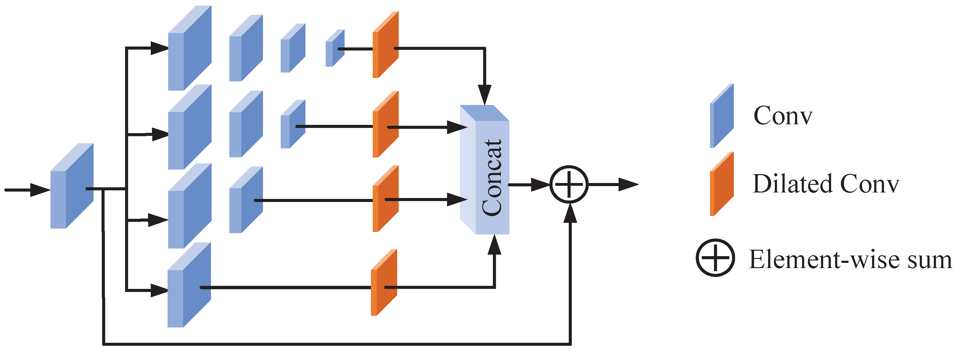
• We propose a more effective shallow feature extraction layer known as the multi-scale feature extraction (MSFE) module, aimed at enhancing the model’s capability to capture low-frequency information. By adjusting the depth and channel number of the convolutional layers of different branches and adding dilated convolutions, the receptive field is expanded and finer-grained shallow features are extracted.
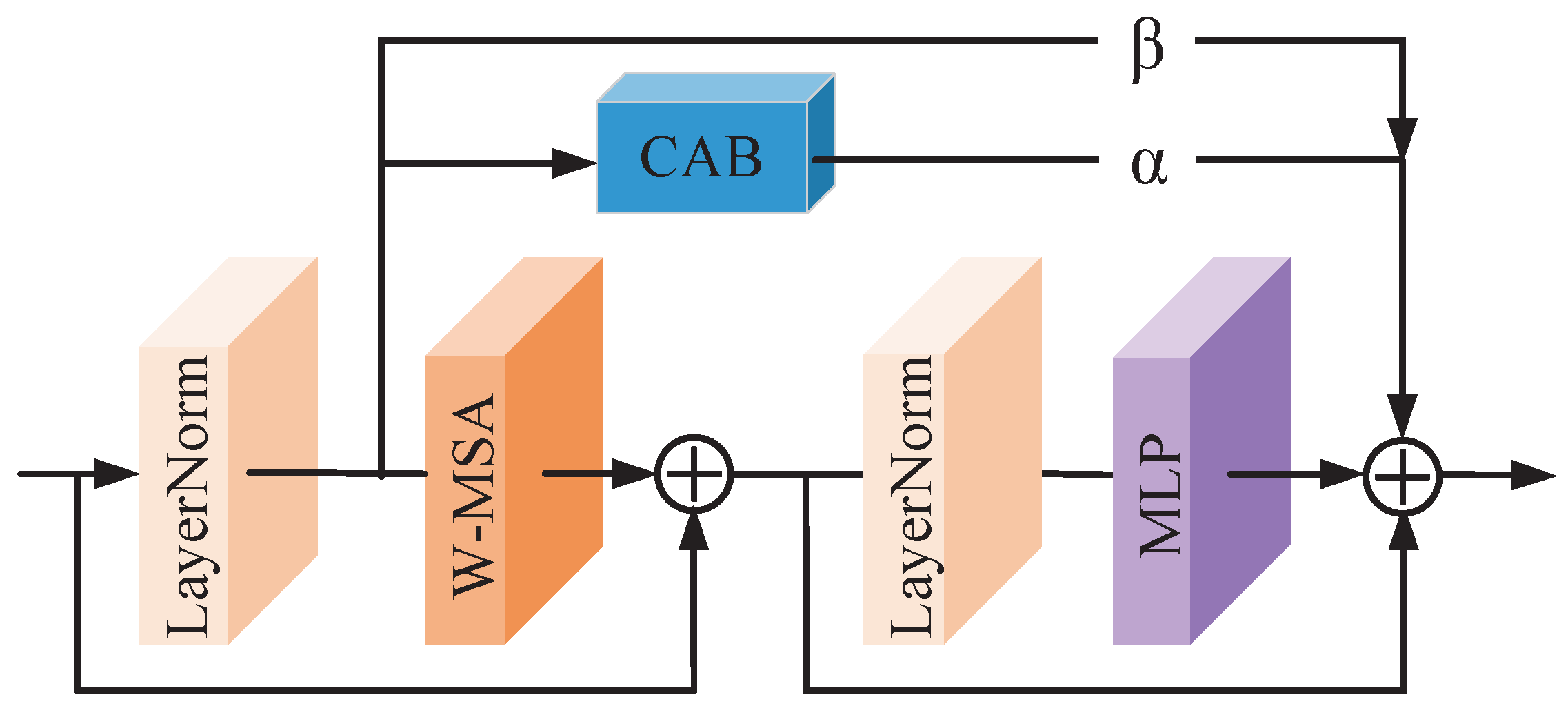
• We analyze the characteristics of window self-attention and propose the fused attention block FAB. Based on moving window multi-head self-attention, we add channel attention through the residual structure to achieve information fusion of global and local features.
• We explore several additional strategies aimed at enhancing the model’s performance. These include employing data augmentation techniques, implementing a smoother Smooth$L_1$ Loss function, enlarging the window size of the swin-transformer, and adopting pre-training strategies.

The subsequent sections of this paper are organized as follows. Section 2 describes the research background for this research methodology. Section 3 describes the overall architecture of the FE-FAIR method. Section 4 introduces the evolution process of FE-FAIR and the experimental results on benchmark tests of performance in different tasks. Section 5 summarizes the contributions of this work.

2. Related Work

In this section, we briefly describe part of the evolution of the image SR method. First, we give an overview of attention mechanism methods and then analyze transformer-based methods.

2.1. Deep Network Methods for Image SR

Since SRCNN [2] first introduced convolutional neural networks into image SR, people have successively proposed a variety of deep network methods [3,5,6,7] to improve the performance of the model, thereby improving the quality of model reconstruction images. For example, sub-pixel convolution techniques [4], deeper networks and residual blocks [5,6], and more complex dense blocks [7] are used to improve the expressive ability of the model. In order to improve the visual quality after image reconstruction, Refs. [23,24] used generative adversarial networks to generate more realistic images. Limited by CNN size effects and feature extraction mechanisms, enhancing the performance of deep convolutional neural networks (CNNs) in image SR tasks becomes increasingly challenging. To solve this problem, some studies integrate attention mechanisms into various layers of CNNs [9,25], allowing for a more detailed understanding and analysis of images at different levels. In addition, researchers also explored techniques to introduce spatial and channel attention into these mechanisms [8,10], aiming to improve model efficiency further. These pioneering efforts provide valuable insights and motivate us to advocate deeper integration of attention mechanisms to effectively capture relevant information between different locations, thereby improving model performance.

2.2. Transformer-Based Methods for Image SR

In recent years, the great success of transformers in natural language processing (NLP) tasks has attracted attention in computer vision. Pure transformer-based methods perform excellently by handling long-distance dependencies well [13,15,26,27,28,29,30]. Some work has shown that combining convolutions and transformers can achieve more advanced results [31,32,33]. SwinIR [16] combines the advantages of convolutions and transformers and proposes a network for tasks such as image SR, which performs well in various image restoration tasks. EDT [17] explores the impact of pre-training mechanisms on transformer methods to enhance the performance of SR networks further. However, these works underestimate shallow feature importance and fail to combine global features with local features effectively. Therefore, our model focuses on more effective shallow feature extraction and feature fusion during the deep feature extraction process, effectively improving the model’s ability to depict image details.

3. Methodology

Inspired by the above work, we propose the FE-FAIR method in this section—the specific network structure shown in Figure 2.

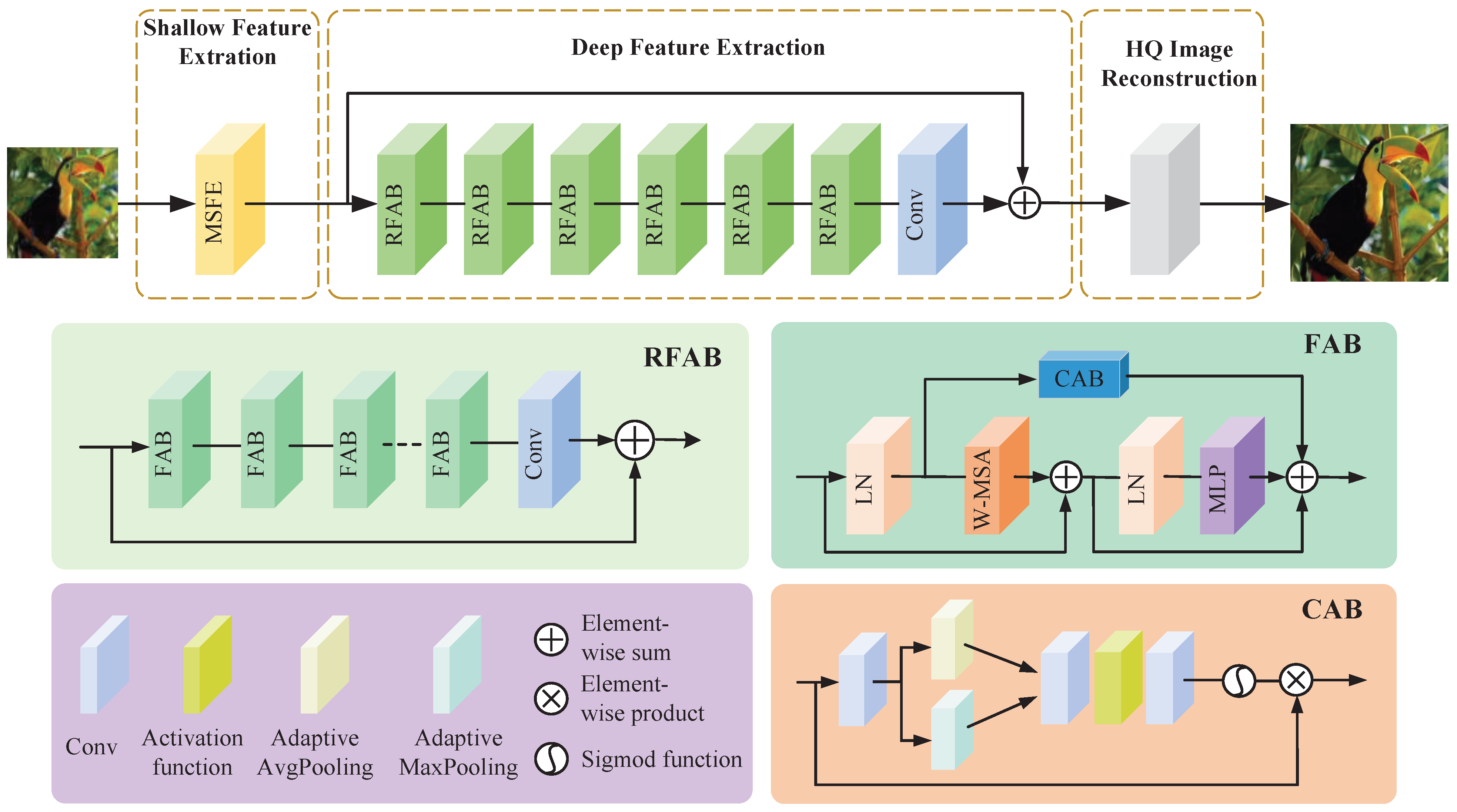
3.1. Network Architecture

FE-FAIR mainly consists of three modules: the shallow feature, deep feature, and graphic reconstruction module. Specifically, the shallow feature module is mainly composed of multi-scale feature extraction layers, using different numbers of convolutional layers and atrous convolution combinations to extract shallow features from different scales. The deep feature extraction module mainly comprises the shifted window self-attention and channel attention mechanisms and introduces the residual structure. The image reconstruction module mainly consists of convolutional and pixel-shuffle layers.

Expressly, for the input low-resolution image $I_{LR}\in {\omega }^{C_0\times H\times W}$, we initially utilize a multi-scale feature extraction (MSFE) module to extract shallow-layer features $F_0\in {\omega }^{C\times H\times W}$ in different dimensions as follows:

$$F_0={\varphi }_{MSFE}\left(I_{LR}\right)$$

(1)

where H and W represent the height and width of the input image, $C_0$ and C represent the number of channels output by the input image and shallow feature extraction layer, respectively, and ${\varphi }_{MSFE}$ represents the MSFE module. The intelligence of the MSFE module is to obtain rich low-frequency feature information from different perspectives and levels. Subsequently, the deep feature extraction module ${\varphi }_{DF}\left(F_0\right)$ is utilized to obtain deep features $F_{DF}\in {\omega }^{C\times H\times W}$:

$$F_{DF}={\varphi }_{DF}\left(F_0\right)$$

(2)

where ${\varphi }_{DF}$ consists of N residual fused attention block (RFAB) and a $3\times 3$ convolutional layer ${\varphi }_{Conv}$. This structure can extract deep features layer by layer, as follows:

$$F_i={\varphi }_{RFABi}\left(F_{i-1}\right),i=1,2,\cdots ,N$$

(3)

$$F_{DF}={\varphi }_{Conv}\left(F_i\right)$$

(4)

where ${\varphi }_{RFABi}$ represents the ith RFAB block. Subsequently, a $3\times 3$ convolutional layer is used after the deep feature extraction layer to aggregate features. Finally, the high-quality image reconstruction module ${\varphi }_{HQ}$ is applied to reconstruct the high-quality image $I_{SR}$, as follows:

$$I_{SR}={\varphi }_{HQ}(F_0+F_{DF})$$

(5)

In order to enhance the stability of the model while effectively retaining the low-frequency and high-frequency information of the image, we use residual connections to transfer the low-frequency information to the image reconstruction block. In the image reconstruction block, we utilize the pixel-shuffle to upsample the reconstructed image.

3.2. Multi-Scale Feature Extraction (MSFE) Module

The shallow feature extraction block mainly maps input features from low latitudes to higher dimensions, usually containing low-frequency information. Convolutional layers perform well in the early processing of visual tasks, thereby facilitating better-optimized results [32]. Simultaneously, we concentrate on the correlation between the target pixel and surrounding pixels, noting that this correlation diminishes as the pixel distance increases. The atrous spatial pyramid pooling (ASPP) [34] uses multiple parallel atrous convolutional layers with different sampling rates to extract features from different scales. Inspired by ASPP, we design the MSFE module based on the concept of multi-scale convolution, with the primary process outlined as follows:

$$F_{in}=H_{Conv1}\left(I_{LR}\right)$$

(6)

$$F_i=H_{branc{h}_i}\left(F_{in}\right),i=1,2,3,4$$

$$F_{concat}=Concate(F_0,F_1,F_2,F_3)$$

$$F_{out}=H_{Conv2}(F_{concat}+F_{in})$$

where $F_{in}$ indicates the mapped high-dimensional features, and $branc{h}_i$ represents dilated convolution modules of different scales. $Conv1$ implements the mapping of input features from low to high dimensions, and $Conv2$ indicates the aggregation of features from different branches.

As illustrated in Figure 3, for the input feature $I_{LR}\in {\omega }^{C_0\times H\times W}$, a convolutional layer is employed to perform feature mapping from low to high dimensions. Subsequently, distinct branches are utilized to acquire features at various scales. Each branch ($branc{h}_i$) comprises varying numbers of convolutional layers and dilated convolutional layers. The dilation value of the dilated convolutional layer corresponds to the number of convolutional layers, where a higher number of convolutional layers entails a larger dilation value [35]. This design effectively expands the receptive field of the convolutional layer while enabling each branch to focus on the interrelation between the central feature and surrounding features across different scales. Ultimately, the information from different branches is concatenated, and a residual structure is employed to incorporate previous level information, thereby enhancing model stability.

3.3. Fused Attention Block (FAB)

The window-based multi-head self-attention mechanism can extract high-frequency information and local features within the feature map. By adding global features, the model can effectively integrate the information from the entire feature map. Previous studies have demonstrated that convolutional layers can enhance the performance of transformers [36]. Channel attention, as proposed by Hu et al. [20], focuses on the importance and correlation of different feature channels. It assigns different weight characteristics to each channel, thereby enhancing model’s capability for global feature extraction. Consequently, the fusion of multi-head self-attention and channel attention serves to amalgamate features effectively. As illustrated in Figure 4, subsequent to passing through the LayerNorm layer, the channel attention block (CAB) and W-MSA operate as parallel structures to calculate the feature map across different dimensions, yielding a residual summation as output. To balance channel attention and W-MSA, we multiply the original input and output features of CAB by the adaptive weights of the sum, respectively. For an input feature X, the entire FAB processing process is as follows:

$$X_{norm}=LN\left(X\right)$$

(7)

$$X_{MSA}=W-MSA\left(X_{norm}\right)+X$$

$$X_T=MLP\left(LN\left(X_{MSA}\right)\right)+X_{MSA}$$

$$X_{out}=X_T+\alpha CAB\left(X_{norm}\right)+\beta X$$

where $X_{norm}$ represents the layernorm (LN) layer, $X_{MSA}$ represents the intermediate result of multi-head self-attention calculation, $X_T$ represents the output feature of W-MSA branch, and $X_{out}$ represents the output feature of the FAB. MLP stands for multi-layer perceptron layer, and CAB stands for channel attention block.

The specific calculation process of the window self-attention mechanism is as follows: given an input feature of size $H\times W\times C$, divide the input feature into non-overlapping windows of size $M^2$, then the total number of windows is $\frac{HW}{M^2}$. The input features can be reshaped into $\frac{HW}{M^2}\times M^2\times C$. Subsequently, self-attention is calculated within each window independently. For each window feature $\in {\Re }^{M^2\times C}$, the query, key, and value matrix are calculated as

$$Q=X{M}_{Q}K=X{M}_{K}V=X{M}_V$$

(8)

where $M_Q$, $M_K$, and $M_V$ represent the mapping matrices of query, key, and value, respectively. Then, the self-attention of the window can be expressed as

$$Attention(Q,K,V)=Softmax(\frac{Q{K}^T}{\sqrt{d}}+B)V$$

(9)

where d represents the dimension of query/key, and B indicates the relative position encoding. In addition, in order to promote information exchange between adjacent windows, the shift window method is also utilized, with the shift size being set at half the window size.

The CAB module mainly consists of convolutional and standard channel attention (CA) layers. The specific structure is shown in Figure 2. Due to the large number of channels, a high computational cost will be incurred when the standard channel attention layer is combined with the transformer. To address this, channels are compressed to $\frac{C}{\gamma }$ while maintaining similar performance using a convolutional layer. The entire CAB calculation process is as follows:

$$X_{out}=CA\left(Conv\left(X_{in}\right)\right)$$

(10)

where $X_{in}$, $X_{out}$, and $Conv$ represent input features, output features, and convolution layer.

As shown in Figure 2, each residual group fused attention block (RFAB) contains N fused attention block (FAB) modules and a $3\times 3$ convolutional layer. Precisely, for the ith RFAB, it can be calculated as

$$F_{i,0}=F_{i-1},i=1,2,\cdots ,N$$

(11)

$$F_{i,j}=H_{FA{B}_{i,j}}\left(F_{i,j-1}\right),j=1,2,\cdots ,M$$

$$F_i=H_{Con{v}_i}\left(F_{i,M}\right)+F_{i,0}$$

where $F_{i,0}$ and $F_i$ represent the input features and output features of the ith RFAB, $H_{FA{B}_{i,j}}$ represents the ith FAB calculation block in the jth RFAB, and $H_{conv}$ represents the convolution layer of the ith RFAB module. This design offers two notable advantages. Firstly, the incorporation of convolutional layers facilitates a more stable aggregation of information. Secondly, the utilization of residual connections not only stabilizes the model’s training but also enhances inter-layer relationships by incorporating information from different modules.

3.4. Loss Function

For previous image SR methods, $L_1$ pixel loss is generally used as the loss function to optimize the model. Under normal circumstances, $L_1$ Loss can obtain better model performance.

$$L_1={\parallel I_{SR}-I_{HQ}\parallel }_1$$

However, the $L_1$ Loss suffers from nondifferentiability at specific points, which can impede loss optimization. Secondly, in the later stage of model training, the difference between the sum and the sum is slight, but its derivative is still a constant. In this way, the loss value will fluctuate around the stable value when the learning rate remains unchanged, making it challenging to achieve higher accuracy. Therefore, we use Smooth$L_1$ Loss [37] as the loss optimization function of the method. Smooth$L_1$ Loss is expressed explicitly as

$$L=\left\{\begin{array}{cc}\frac{0.5{(I_{SR}-I_{HQ})}^2}{\theta }\hfill & if|I_{SR}-I_{HQ}|<\theta \hfill \\ |I_{SR}-I_{HQ}|-0.5\theta \hfill & otherwise\hfill \end{array}\right.$$

(12)

where $\theta$ is set to 1 by default in our method. As indicated by the formula above, Smooth$L_1$ Loss employs the form of $L_1$ Loss when $|I_{SR}-I_{HQ}|⩾\theta$ and uses the form of $L_2$ loss when $|I_{SR}-I_{HQ}|<\theta$. This approach effectively addresses issues such as gradient explosion arising from significant losses and accuracy concerns when losses are small.

4. Experiments

In this section, the FE-FAIR method proposed in this paper is compared with other state-of-the-art methods, such as EDSR [6], RCAN [8], SAN [10], IGNN [38], HAN [9], NLSN [25], SwinIR [16], EDT [17], CARN [39], IMDN [40], LAPAR-A [41], LatticeNet [42], BM3D [43], WNNM [44], DnCNN [45], IRCNN [46], FFDNet [47], NLRN [48], FOCNet [49], MWCNN [50], DRUNet [51], DSNet [52], RPCNN [53], BRDNet [54], and IPT [15].

Simultaneously, the peak signal-to-noise ratio (PSNR) and structural similarity (SSIM) [55] are utilized for evaluation. The calculation process of PSNR is demonstrated as follows:

$$PSNR=10\times {log}_{10}\frac{Ma{x}^2}{MSE}=20\times {log}_{10}\frac{Max}{\sqrt{MSE}}$$

where the default value of $Max$ is 255. The calculation expression of mean square error (MSE) is presented as follows:

$$MSE=\frac{1}{M\times N}\sum _{i=1}^M\sum _{j=1}^N{(I_{HR}(i,j)-I_{SR}(i,j))}^2$$

where H and W are the number of pixels in the length and width of the image, respectively. The value of PSNR depends on MSE, so the smaller the MSE, the greater the PSNR value, which means the smaller the difference between the reconstructed image and the actual image. The SSIM is also used to measure the similarity between the reconstructed and authentic images from brightness, contrast, and structure. SSIM can be expressed as

$$SSIM=\frac{(2{\mu }_{I_{HR}}\times {\mu }_{I_{SR}}+C_1)(2{\sigma }_{I_{HR}}\times {\sigma }_{I_{SR}}+C_2)}{({\mu }_{I_{HR}}^2+{\mu }_{I_{SR}}^2+C_1)({\sigma }_{I_{HR}}^2+{\sigma }_{I_{SR}}^2+C_2)}$$

where ${\mu }_{I_{HR}}$, ${\mu }_{I_{SR}}$, ${\sigma }_{I_{HR}}$, ${\sigma }_{I_{SR}}$, ${\zeta }_{I_{HR}}$, and ${\zeta }_{I_{SR}}$ represent the mean, standard deviation, and covariance of $I_{HR}$ and $I_{SR}$, respectively. $C_1$ and $C_2$ are constants. The closer the value of $SSIM$ is to 1, the higher the similarity between the two images.

All experiments are conducted using PyTorch version 2.0 on 4 NVIDIA Tesla V100 GPUs with CUDA version 12.2.

4.1. Experimental Setup

In classical image SR, the DF2K dataset (comprising DIV2K [22] with 900 images and Flickr2K [22] with 2650 images) containing 3550 images is utilized as the original training set. Bicubic downsampling with scaling factors of $\times 2$, $\times 3$, and $\times 4$ are performed using MATLAB to generate low-resolution images. The test set includes popular super-resolution benchmark datasets such as Set5 [56], Set14 [57], BSD100 [58], Urban100 [59], and Manga109 [60]. Regarding the architecture of FE-FAIR, the parameters are configured as follows: the number of RFABs, FABs, channels, attention heads, and window size are set to 6, 6, 180, 6, and 16, respectively. In lightweight image SR tasks, these parameters are set to 4, 6, 60, 6, and 16, respectively. The channel compression parameter $\gamma$ in the MSFE module is defaulted to 3 for classical tasks and 6 for lightweight tasks. The channel compression parameter $\gamma$ in CAB is set to 5, and $\alpha$ and $\delta$ in FAB are treated as adaptive parameters.

For image denoising, the training set comprises DIV2K (900 images), Flickr2K (2650 images), WED [61] (4744 images), and BSD200 [58] (200 images). The test set includes Set12 [45], BSD68 [58], CBSD68 [58], Kodak24 [62], McMaster [63], and Urban100 datasets. The parameter configurations remain consistent with classic SR.

For classical SR, we set the batch size to 32 and the total training iterations to 500 k. The initial learning rate is $2\times {10}^{-4}$, and it is halved at iterations [250 k, 400 k, 450 k, 475 k, 500 k], respectively. For lightweight SR, the batch size is 64, and the total number of training iterations is also 500 k. For the image denoising task, the batch size is 8, and the total number of training iterations is 1500 k. The initial learning rate is $2\times {10}^{-4}$, halved at iterations [600 k, 1000 k, 1300 k, 1450 k], respectively. For the pre-training model, 1.2 million images from ImageNet [21] are used for 1000 k iterations. The initial learning rate is also $2\times {10}^{-4}$, halved at iterations [300 k, 500 k, 750 k, 900 k, 1000 k]. Subsequently, the DF2K dataset (DIV2K with 900 images + Flickr2K with 2650 images) is employed for fine-tuning with 250 k iterations. The learning rate is initialized to $2\times {10}^{-5}$ and halved at iterations [130 k, 200 k, 230 k, 245 k, 250 k].

Simultaneously, to determine the optimal number of iterations in our proposed method, experiments are conducted on the DF2K dataset, and results are shown in Figure 5. We can observe that after 500 k iterations, the method converges in both tasks. Specifically, compared with classic tasks, the lightweight SR methods can enter the convergence state faster due to the smaller number of parameters and minor computational cost, and the indicators are more stable during the training process. The classic task method has better performance. Therefore, we set 500 k iterations in this work as the total training times.

4.2. Ablation Experiment

In this part of the work, the impact of a series of methods proposed in this paper on image SR are separately verified.

4.2.1. Effectiveness of MSFE

Rich shallow features can help the model retain sufficient low-frequency information [64] while providing more effective feature information for the deep feature extraction module. The MSFE module combines dilated convolutions with different numbers of convolutional layers to achieve more detailed feature capture. The effectiveness of the proposed MSFE module is demonstrated through experimental setups in our work. Using the traditional single-layer convolutional layer as the baseline, this part of the work tests the method gain of three convolutional layers, ASPP, and MSFE modules as shallow feature extraction layers. The results are quantified on Set14, Urban100, and Manga109. As shown in

Table 1. The effects of different shallow feature extraction modules. Bold text and numbers indicate the method we used and the best results among all methods.

Module	Scale	Set14 [57]	Urban100 [59]	Manga109 [60]
Conv	2	34.46/0.9250	33.81/0.9427	39.92/0.9797
3 × Conv	2	34.47/0.9252	33.82/0.9428	39.93/0.9796
ASPP [34]	2	34.48/0.9253	33.84/0.9431	39.94/0.9798
MSFE	2	34.52/0.9257	33.92/0.9435	39.98/0.9804
Conv	4	29.09/0.7950	27.45/0.8254	32.03/0.9260
3 × Conv	4	29.10/0.7949	27.47/0.8256	32.05/0.9259
ASPP [34]	4	29.12/0.7952	27.48/0.8259	32.07/0.9262
MSFE	4	29.15/0.7958	27.53/0.8271	32.11/0.9265

, when using MSFE as the shallow feature extraction layer, the network achieves a performance gain of 0.06 to 0.11 dB compared to other methods, demonstrating a significant improvement over alternative methods. All results show that MSFE can effectively improve the performance of SR methods.

4.2.2. Effects of the FAB

The FAB module combines self-attention and channel attention mechanisms through residual connections, enabling the integration of global features into local features. We conducted experiments to demonstrate the effectiveness of the FAB module.

Table 2. The effects of the FAB module on performance. Bold text and numbers indicate the method we used and the best results among all methods.

Module	Set14 [57]	Urban100 [59]	Manga109 [60]
STL	29.15/0.7958	27.53/0.8271	32.11/0.9265
FAB	29.17/0.7959	27.62/0.8277	32.17/0.9270
FAB + $\alpha$ + $\beta$	29.19/0.7960	27.65/0.8282	32.20/0.9273

presents the quantitative performance on the Set14, Urban100, and Manga109 test sets for $\times 4$ super-resolution. Compared to the baseline performance of the STL module in SwinIR, the FAB module brings a performance gain of 0.05 to 0.09 dB. Adaptive weights $\alpha$ and $\beta$ are set to avoid conflicts between channel attention and window self-attention. We further investigate the impact of these variable weights on model performance. Experiments show that without adding parameters, the inclusion of $\alpha$ and $\beta$ results in a performance gain of 0.03 dB based on the FAB module. This indicates that the adaptive parameters $\alpha$ and $\beta$ reduce negative impacts between different attention mechanisms, facilitating their fusion and enabling improved model performance.

4.2.3. Effects of Smooth$L_1$

Loss Smooth$L_1$ Loss offers smoother convergence and better performance compared to traditional $L_1$ Loss. To demonstrate the superiority of Smooth$L_1$ Loss as a loss function, experiments were conducted.

Table 3. The effects of using different loss functions on performance. Bold text and numbers indicate the method we used and the best results among all methods.

Module	${\mathit{L}}_1$ Loss	Smooth${\mathit{L}}_1$ Loss
PSNR/SSIM	27.65/0.8282	27.68/0.8289

presents the quantitative results for the super-resolution task with a scaling factor of $\times 4$ on the Urban100 dataset. Smooth$L_1$ Loss achieves a performance gain of 0.03 dB compared to $L_1$ Loss. These results indicate that Smooth$L_1$ Loss, when used as a loss function for image super-resolution tasks, enhances the model’s performance.

4.2.4. Effects of Window Size

EDT explored the impact of window size on the performance of the window self-attention mechanism. It has been proved that increasing the window size is a direct method of improving the performance of the SR network. However, previous studies only explored windows up to 12 × 12 in size. Therefore, we also examined the impact of larger window sizes on network performance.

Table 4. The effects of window size. Bold text and numbers indicate the method we used and the best results among all methods.

Window Size	Set14 [57]	Urban100 [59]	Manga109 [60]
	PSNR/SSIM	PSNR/SSIM	PSNR/SSIM
(8, 8)	29.20/0.7962	27.68/0.8289	32.23/0.9268
(12, 12)	29.22/0.7966	27.87/ 0.8348	32.28/0.9279
(16, 16)	29.21/0.7966	27.96/0.8377	32.32/0.9287

shows the quantitative test results when the amplification factor is 4 on the Set14, Urban100, and Manga109 test sets. We can find from the results that when the window size is 16, the model’s performance can be effectively improved, especially the PSNR improvement on Urban100, which reaches 0.24 dB. Therefore, in FE-FAIR, we directly set the window size to 16.

4.3. Comparison Result

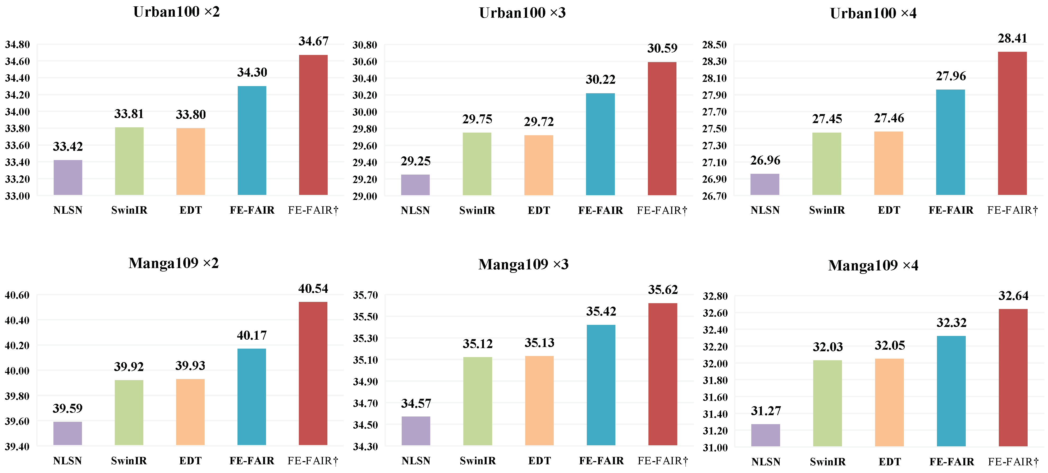
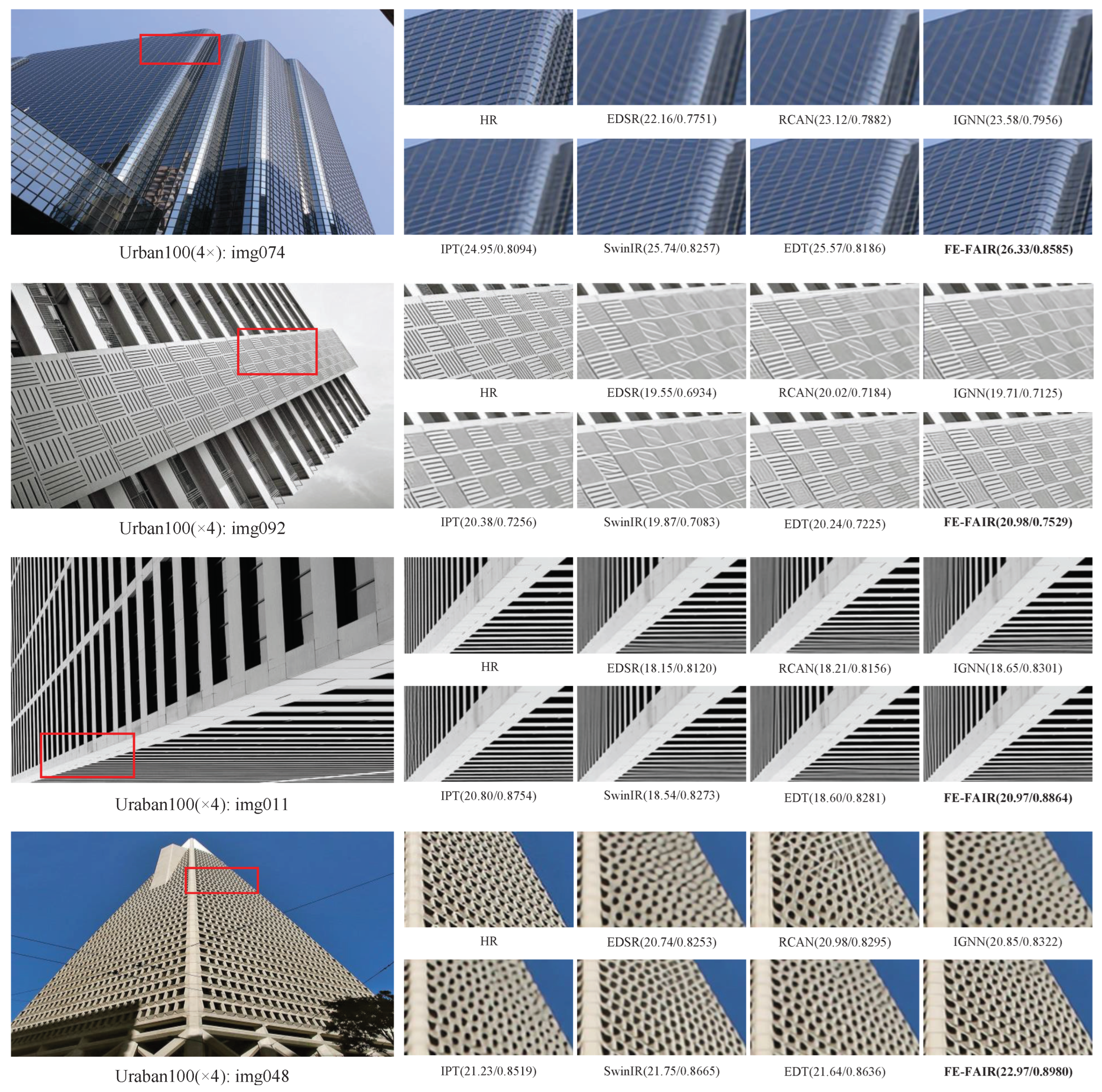
4.3.1. Results on Classical Image Super-Resolution

Quantitative comparison. 

Table 5. Quantitative comparison with state-of-the-art methods (average PSNR/SSIM) for classical image SR on benchmark datasets. The best and second-best performances are bolded and underlined, respectively. “†” indicates we use a pre-training strategy on ImageNet.

Method	Scale	Training	Set5 [56]	Set14 [57]	BSD100 [58]	Urban100 [59]	Manga109 [60]
			PSNR/SSIM	PSNR/SSIM	PSNR/SSIM	PSNR/SSIM	PSNR/SSIM
EDSR [6]	×2	DIV2K	38.11/0.9602	33.92/0.9195	32.32/0.9013	32.93/0.9351	39.10/0.9773
RCAN [8]	×2	DIV2K	38.27/0.9614	34.12/0.9216	32.41/0.9027	33.34/0.9384	39.44/0.9786
SAN [10]	×2	DIV2K	38.31/0.9620	34.07/0.9213	32.42/0.9028	33.10/0.9370	39.32/0.9792
IGNN [38]	×2	DIV2K	38.24/0.9613	34.07/0.9217	32.41/0.9025	33.23/0.9383	39.35/0.9786
HAN [9]	×2	DIV2K	38.27/0.9614	34.16/0.9217	32.41/0.9027	33.35/0.9385	39.46/0.9785
NLSN [25]	×2	DIV2K	38.34/0.9618	34.08/0.9231	32.43/0.9027	33.42/0.9394	39.59/0.9789
SwinIR [16]	×2	DF2K	38.42/0.9623	34.46/0.9250	32.53/0.9041	33.81/0.9427	39.92/0.9797
EDT [17]	×2	DF2K	38.45/0.9624	34.57/0.9263	32.52/0.9041	33.80/0.9425	39.93/0.9800
FE-FAIR	×2	DF2K	38.58/0.9629	34.73/0.9266	32.58/0.9048	34.30/0.9460	40.17/0.9804
IPT † [15]	×2	ImageNet	38.37/-	34.43/-	32.48/-	33.76/-	-/-
EDT † [17]	×2	DF2K	38.63/0.9632	34.80/0.9273	32.62/0.9052	34.27/0.9456	40.37/0.9811
FE-FAIR †	×2	DF2K	38.66/0.9632	34.99/0.9275	32.66/0.9057	34.67/0.9490	40.54/0.9812
EDSR [6]	×3	DIV2K	34.65/0.9280	30.52/0.8462	29.25/0.8093	28.80/0.8653	34.17/0.9476
RCAN [8]	×3	DIV2K	34.74/0.9299	30.65/0.8482	29.32/0.8111	29.09/0.8702	34.44/0.9499
SAN [10]	×3	DIV2K	34.75/0.9300	30.59/0.8476	29.33/0.8112	28.93/0.8671	34.30/0.9494
IGNN [38]	×3	DIV2K	34.72/0.9298	30.66/0.8484	29.31/0.8105	29.03/0.8696	34.39/0.9496
HAN [9]	×3	DIV2K	34.75/0.9299	30.67/0.8483	29.32/0.8110	29.10/0.8705	34.48/0.9500
NLSN [25]	×3	DIV2K	34.85/0.9306	30.70/0.8485	29.34/0.8117	29.25/0.8760	34.57/0.9508
SwinIR [16]	×3	DF2K	34.97/0.9318	30.93/0.8534	29.46/0.8145	29.75/0.8826	35.12/ 0.9537
EDT [17]	×3	DF2K	34.97/0.9316	30.89/0.8527	29.44/0.8142	29.72/0.8814	35.13/0.9534
FE-FAIR	×3	DF2K	35.02/0.9326	31.02/0.8551	29.50/0.8162	30.22/0.8898	35.42/0.9547
IPT † [15]	×3	ImageNet	38.37/-	34.43/-	32.48/-	33.76/-	-/-
EDT † [17]	×3	DF2K	35.13/0.9328	31.09/0.8553	29.53/0.8165	30.07/0.8863	35.47/0.9550
FE-FAIR †	×3	DF2K	35.14/0.9335	31.24/0.8569	29.53/0.8172	30.59/0.8944	35.62/0.9561
EDSR [6]	×4	DIV2K	32.46/0.8968	28.80/0.7876	27.71/0.7420	26.64/0.8033	31.02/0.9148
RCAN [8]	×4	DIV2K	32.63/0.9002	28.87/0.7889	27.77/0.7436	26.82/0.8087	31.22/0.9173
SAN [10]	×4	DIV2K	32.64/0.9003	28.92/0.7888	27.78/0.7436	26.79/0.8068	31.18/0.9169
IGNN [38]	×4	DIV2K	32.57/0.8998	28.85/0.7891	27.77/0.7434	26.84/0.8090	31.28/0.9182
HAN [9]	×4	DIV2K	32.64/0.9002	28.90/0.7890	27.80/0.7442	26.85/0.8094	31.42/0.9177
NLSN [25]	×4	DIV2K	32.59/0.9000	28.87/0.7891	27.78/0.7444	26.96/0.8109	31.27/0.9184
SwinIR [16]	×4	DF2K	32.92/0.9044	29.09/0.7950	27.92/0.7489	27.45/ 0.8254	32.03/0.9260
EDT [17]	×4	DF2K	32.82/0.9031	29.09/0.7939	27.91/0.7483	27.46 /0.8246	32.05/0.9254
FE-FAIR	×4	DF2K	33.05/0.9053	29.21/0.7966	27.97/0.7514	27.96/0.8377	32.32/0.9287
IPT † [15]	×4	ImageNet	38.37/-	34.43/-	32.48/-	33.76/-	-/-
EDT † [17]	×4	DF2K	33.06/0.9055	29.23/0.7971	27.99/0.7510	27.75/0.8317	32.39/0.9283
FE-FAIR †	×4	DF2K	33.19/0.9075	29.35/0.7992	28.03/0.7531	28.41/0.8450	32.64/0.9301

shows the quantitative comparison results between FE-FAIR and other state-of-the-art methods: EDSR [6], RCAN [8], SAN [10], IGNN [38], HAN [9], NLSN [25], SwinIR [16], and EDT [17]. We can see that FE-FAIR exhibits the best performance across all test sets and magnifications. Specifically, FE-FAIR achieves a performance gain of 0.33–0.55 dB on Urban100 and 0.27–0.34 dB on Manga109. Thus, FE-FAIR demonstrates superior performance in image super-resolution. Additionally, we present quantitative comparison results between the pre-training strategy FE-FAIR and state-of-the-art models IPT† [15] and EDT† [17]. The pre-trained model exhibits a substantial performance improvement, notably surpassing the baseline (SwinIR) by 0.8 dB on Urban100, thereby affirming the effectiveness of the pre-training strategy.

Visual Comparison. We selected several pictures (img011, img048, image074, image092) from the benchmark to show the super-resolution reconstruction results of the model. It can be found from Figure 6 that our results have greatly improved texture details and authenticity.

4.3.2. Results on Lightweight Image Super-Resolution

Quantitative comparison. 

Table 6. Quantitative comparison (average PSNR/SSIM) with state-of-the-art methods for lightweight image SR on benchmark datasets. The best and second-best performances are bolded and underlined, respectively.

Method	Scale	# Params	Set5 [56]	Set14 [57]	B100 [58]	Urban100 [59]	Manga109 [60]
			PSNR/SSIM	PSNR/SSIM	PSNR/SSIM	PSNR/SSIM	PSNR/SSIM
CARN [39]	×2	1592 k	37.76/0.9590	33.52/0.9166	32.09/0.8978	31.92/0.9256	38.36/0.9765
IMDN [40]	×2	548 k	38.00/0.9605	33.63/0.9177	32.19/0.8996	32.17/0.9283	38.88/0.9774
LAPAR-A [41]	×2	548 k	38.01/0.9605	33.62/0.9183	32.19/0.8999	32.10/0.9283	38.67/0.9772
LatticeNet [42]	×2	756 k	38.15/0.9610	33.78/0.9193	32.25/0.9005	32.43/0.9302	-/-
SwinIR [16]	×2	878 k	38.14/0.9611	33.86/0.9206	32.31/0.9012	32.76/0.9340	39.12/0.9783
EDT [17]	×2	917 k	38.23/0.9615	33.99/0.9209	32.37/0.9021	32.98/0.9362	39.45/0.9789
FE-FAIR	×2	2291 k	38.30/0.9621	33.10/0.9214	32.41/0.9027	33.37/0.9417	39.56/0.9808
CARN [39]	×3	1592 k	34.29/0.9255	30.29/0.8407	29.06/0.8034	28.06/0.8493	33.50/0.9440
IMDN [40]	×3	703 k	34.36/0.9270	30.32/0.8417	29.09/0.8046	28.17/0.8519	33.61/0.9445
LAPAR-A [41]	×3	544 k	34.36/0.9267	30.34/0.8421	29.11/0.8054	28.15/0.8523	33.51/0.9441
LatticeNet [42]	×3	765 k	34.53/0.9281	30.39/0.8424	29.15/0.8059	28.33/0.8538	-/-
SwinIR [16]	×3	886 k	34.62/0.9289	30.54/0.8463	29.20/0.8082	28.66/0.8624	33.98/0.9478
EDT [17]	×3	919 k	34.73/0.9299	30.66/0.8481	29.29/0.8103	28.89/0.8674	34.44/0.9498
FE-FAIR	×3	2299 k	34.80/0.9311	30.75/0.8492	29.33/0.8105	29.25/0.8727	34.52/0.9518
CARN [39]	×4	1592 k	32.13/0.8937	28.60/0.7806	27.58/0.7349	26.07/0.7837	30.47/0.9084
IMDN [40]	×4	715 k	32.21/0.8948	28.58/0.7811	27.56/0.7353	26.04/0.7838	30.45/0.9075
LAPAR-A [41]	×4	659 k	32.15/0.8944	28.61/0.7818	27.61/0.7366	26.14/0.7871	30.42/0.9074
LatticeNet [42]	×4	777 k	32.30/0.8962	28.68/0.7830	27.62/0.7367	26.25/0.7873	-/-
SwinIR [16]	×4	897 k	32.44/0.8976	28.77/0.7858	27.69/0.7406	26.47/0.7980	30.92/0.9151
EDT [17]	×4	922 k	32.53/0.8991	28.88/0.7882	27.76/0.7433	26.71/0.8051	31.35/0.9180
FE-FAIR	×4	2310 k	32.59/0.9002	28.97/0.7903	27.79/0.7447	27.04/0.8139	31.41/0.9199

shows the quantitative performance comparison results between lightweight FE-FAIR and state-of-the-art lightweight methods: CARN [39], IMDN [40], LAPAR-A [41], LatticeNet [42], SwinIR [16], and EDT [17]. The total number of parameters in our method (evaluated on 1280 × 720 images) is also provided. As shown in Table 6, the quantification performance of FE-FAIR is significantly better than other methods, especially in SSIM. It proves that our method is effective in lightweight image super-resolution tasks.

4.3.3. Results on Image Denoising

We further explore the performance of our method in image denoising. We show the comparison results of FE-FAIR on grayscale and colour image denoising tasks with other state-of-the-art methods: BM3D [43], WNNM [44], DnCNN [45], IRCNN [46], FFDNet [47], NLRN [48], FOCNet [49], MWCNN [50], DRUNet [51], DSNet [52], RPCNN [53], BRDNet [54], IPT, and SwinIR [16].

Table 7. Quantitative comparison (average PSNR) with state-of-the-art models for grayscale image denoising on benchmark datasets. The best and second-best performances are bolded and underlined.

Dataset	$\mathit{\sigma }$	BM3D [43]	WNNM [44]	DnCNN [45]	IRCNN [46]	FFDNet [47]	NLRN [48]	FOCNet [49]	MWCNN [50]	DRUNet [51]	SwinIR [16]	FE-FAIR
Set12 [45]	15	32.37	32.70	32.86	32.76	32.75	33.16	33.07	33.15	33.25	33.36	33.41
	25	29.97	30.28	30.44	30.37	30.43	30.80	30.73	30.79	30.94	31.01	31.07
	50	26.72	27.05	27.18	27.12	27.32	27.64	27.68	27.74	27.90	27.91	27.96
BSD68 [58]	15	31.08	31.37	31.73	31.63	31.63	31.88	31.83	31.86	31.91	31.97	32.04
	25	28.57	28.83	29.23	29.15	29.19	29.41	29.38	29.41	29.48	27.50	27.54
	50	25.60	25.87	26.23	26.19	26.29	26.47	26.50	26.53	26.59	26.58	26.61
Urban100 [59]	15	32.35	32.97	32.64	32.46	32.40	33.45	33.15	33.17	33.44	33.70	33.81
	25	29.70	30.39	29.95	29.80	29.90	30.94	30.64	30.66	31.11	31.30	33.45
	50	25.95	26.83	26.26	26.22	26.50	27.49	27.40	27.42	27.96	27.98	28.12

and

Table 8. Quantitative comparison (average PSNR) with state-of-the-art methods for colour image denoising on benchmark datasets. The best and second-best performances are bolded and underlined.

Dataset	$\mathit{\sigma }$	BM3D [43]	DnCNN [45]	IRCNN [46]	FFDNet [47]	DSNet [52]	RPCNN [53]	BRDNet [54]	IPT [15]	DRUNet [51]	SwinIR [16]	FE-FAIR
CBSD68 [58]	15	33.52	33.90	33.86	33.87	33.91	-	34.10	-	34.30	34.42	34.46
	25	30.71	31.24	31.16	31.21	31.28	31.24	31.43	-	31.69	31.78	31.81
	50	27.38	27.95	27.86	27.96	28.05	28.06	28.16	28.39	28.51	28.56	28.58
Kodak24 [62]	15	34.28	34.60	34.69	34.63	34.63	-	34.88	-	35.31	35.34	35.39
	25	32.15	32.14	32.18	32.13	32.16	32.34	32.41	-	32.89	32.89	32.97
	50	28.46	28.95	28.93	28.98	29.05	29.25	29.22	29.64	29.86	29.79	29.91
McMaster [63]	15	34.06	33.45	34.58	34.66	34.67	-	35.08	-	35.40	35.61	35.67
	25	31.66	31.52	32.18	32.35	32.40	32.33	32.75	-	33.14	33.20	33.31
	50	28.51	28.62	28.91	29.18	29.28	29.33	29.52	29.98	30.08	30.22	30.27
Urban100 [59]	15	33.93	32.98	33.78	33.83	-	-	34.42	-	34.81	35.13	35.26
	25	31.36	30.81	31.20	31.40	-	31.81	31.99	-	32.60	32.90	33.06
	50	27.93	27.59	27.70	28.05	-	28.62	28.56	29.71	29.61	29.82	30.12

provide quantitative comparison results at noise levels of 15, 25, and 50. Specifically, our method outperforms the state-of-the-art method SwinIR by 0.2 dB on the Urban100 benchmark dataset.

5. Conclusions

In this paper, we re-explore the importance of shallow features and propose a multi-scale shallow feature extraction module MSFE to obtain more prosperous and influential low-frequency features. Concurrently, we integrate window self-attention and channel attention in the form of residual connection, proposing the fused attention module FAB. The FAB effectively achieves an effective combination of local feature information and global feature information. In addition, we also incorporate other techniques to improve the model’s performance, such as data augmentation and increasing the window size. Combining these methods, we propose an image super-resolution reconstruction method FE-FAIR. Comparative evaluations on benchmark datasets demonstrate FE-FAIR’s superior performance compared to other state-of-the-art image super-resolution methods. Additionally, our method exhibits better performance in image denoising tasks.

In the future, we will continue exploring further interactions between shallow and deep features to achieve more fine-grained shallow feature capture. Additionally, investigating the impact of various attention fusion methods on image super-resolution remains a promising avenue of research. Due to the enormous potential of the transformer architecture, we aim to further explore its applications across various tasks, including the field of image SR.

References

1. Park, S.C.; Park, M.K.; Kang, M.G. Super-resolution image reconstruction: A technical overview. IEEE Signal Process. Mag. 2003, 20, 21–36. [Google Scholar] [CrossRef]
2. Dong, C.; Loy, C.C.; He, K.; Tang, X. Learning a deep convolutional network for image super-resolution. In Proceedings of the Computer Vision—ECCV 2014: 13th European Conference, Zurich, Switzerland, 6–12 September 2014; Proceedings, Part IV 13. Springer: Cham, Switzerland, 2014; pp. 184–199. [Google Scholar]
3. Dong, C.; Loy, C.C.; Tang, X. Accelerating the super-resolution convolutional neural network. In Proceedings of the Computer Vision—ECCV 2016: 14th European Conference, Amsterdam, The Netherlands, 11–14 October 2016; Proceedings, Part II 14. Springer: Cham, Switzerland, 2016; pp. 391–407. [Google Scholar]
4. Shi, W.; Caballero, J.; Huszár, F.; Totz, J.; Aitken, A.P.; Bishop, R.; Rueckert, D.; Wang, Z. Real-time single image and video super-resolution using an efficient sub-pixel convolutional neural network. In Proceedings of the IEEE Conference on Computer Vision and Pattern Recognition, Las Vegas, NV, USA, 27–30 June 2016; pp. 1874–1883. [Google Scholar]
5. Kim, J.; Lee, J.K.; Lee, K.M. Accurate image super-resolution using very deep convolutional networks. In Proceedings of the IEEE Conference on Computer Vision and Pattern Recognition, Las Vegas, NV, USA, 27–30 June 2016; pp. 1646–1654. [Google Scholar]
6. Lim, B.; Son, S.; Kim, H.; Nah, S.; Mu Lee, K. Enhanced deep residual networks for single image super-resolution. In Proceedings of the IEEE Conference on Computer Vision and Pattern Recognition Workshops, Honolulu, HI, USA, 21–26 July 2017; pp. 136–144. [Google Scholar]
7. Huang, G.; Liu, Z.; Van Der Maaten, L.; Weinberger, K.Q. Densely connected convolutional networks. In Proceedings of the IEEE Conference on Computer Vision and Pattern Recognition, Honolulu, HI, USA, 21–26 July 2017; pp. 4700–4708. [Google Scholar]
8. Zhang, Y.; Li, K.; Li, K.; Wang, L.; Zhong, B.; Fu, Y. Image super-resolution using very deep residual channel attention networks. In Proceedings of the European Conference on Computer Vision (ECCV), Munich, Germany, 8–14 September 2018; pp. 286–301. [Google Scholar]
9. Niu, B.; Wen, W.; Ren, W.; Zhang, X.; Yang, L.; Wang, S.; Zhang, K.; Cao, X.; Shen, H. Single image super-resolution via a holistic attention network. In Proceedings of the Computer Vision–ECCV 2020: 16th European Conference, Glasgow, UK, 23–28 August 2020; Proceedings, Part XII 16. Springer: Cham, Switzerland, 2020; pp. 191–207. [Google Scholar]
10. Dai, T.; Cai, J.; Zhang, Y.; Xia, S.T.; Zhang, L. Second-order attention network for single image super-resolution. In Proceedings of the IEEE/CVF Conference on Computer Vision and Pattern Recognition, Long Beach, CA, USA, 18–24 June 2019; pp. 11065–11074. [Google Scholar]
11. Vaswani, A.; Shazeer, N.; Parmar, N.; Uszkoreit, J.; Jones, L.; Gomez, A.N.; Kaiser, Ł.; Polosukhin, I. Attention is all you need. Adv. Neural Inf. Process. Syst. 2017, 30, 15. [Google Scholar]
12. Dosovitskiy, A.; Beyer, L.; Kolesnikov, A.; Weissenborn, D.; Zhai, X.; Unterthiner, T.; Dehghani, M.; Minderer, M.; Heigold, G.; Gelly, S.; et al. An image is worth 16x16 words: Transformers for image recognition at scale. arXiv 2020, arXiv:2010.11929. [Google Scholar]
13. Carion, N.; Massa, F.; Synnaeve, G.; Usunier, N.; Kirillov, A.; Zagoruyko, S. End-to-end object detection with transformers. In Proceedings of the European Conference on Computer Vision, Glasgow, UK, 23–28 August 2020; Springer: Cham, Switzerland, 2020; pp. 213–229. [Google Scholar]
14. Liu, Z.; Lin, Y.; Cao, Y.; Hu, H.; Wei, Y.; Zhang, Z.; Lin, S.; Guo, B. Swin transformer: Hierarchical vision transformer using shifted windows. In Proceedings of the IEEE/CVF International Conference on Computer Vision, Paris, France, 10–17 October 2021; pp. 10012–10022. [Google Scholar]
15. Chen, H.; Wang, Y.; Guo, T.; Xu, C.; Deng, Y.; Liu, Z.; Ma, S.; Xu, C.; Xu, C.; Gao, W. Pre-trained image processing transformer. In Proceedings of the IEEE/CVF Conference on Computer Vision and Pattern Recognition, Nashville, TN, USA, 20–25 June 2021; pp. 12299–12310. [Google Scholar]
16. Liang, J.; Cao, J.; Sun, G.; Zhang, K.; Van Gool, L.; Timofte, R. Swinir: Image restoration using swin transformer. In Proceedings of the IEEE/CVF International Conference on Computer Vision, Montreal, QC, Canada, 10–17 October 2021; pp. 1833–1844. [Google Scholar]
17. Li, W.; Lu, X.; Qian, S.; Lu, J.; Zhang, X.; Jia, J. On efficient transformer-based image pre-training for low-level vision. arXiv 2021, arXiv:2112.10175. [Google Scholar]
18. Lu, Z.; Li, J.; Liu, H.; Huang, C.; Zhang, L.; Zeng, T. Transformer for single image super-resolution. In Proceedings of the IEEE/CVF Conference on Computer Vision and Pattern Recognition, New Orleans, LA, USA, 18–24 June 2022; pp. 457–466. [Google Scholar]
19. Chen, X.; Wang, X.; Zhou, J.; Qiao, Y.; Dong, C. Activating more pixels in image super-resolution transformer. In Proceedings of the IEEE/CVF Conference on Computer Vision and Pattern Recognition, Vancouver, BC, Canada, 17–24 June 2023; pp. 22367–22377. [Google Scholar]
20. Hu, J.; Shen, L.; Sun, G. Squeeze-and-excitation networks. In Proceedings of the IEEE Conference on Computer Vision and Pattern Recognition, Salt Lake City, UT, USA, 18–23 June 2018; pp. 7132–7141. [Google Scholar]
21. Deng, J. A large-scale hierarchical image database. In Proceedings of the IEEE Computer Vision and Pattern Recognition, Miami, FL, USA, 20–25 June 2009. [Google Scholar]
22. Agustsson, E.; Timofte, R. Ntire 2017 challenge on single image super-resolution: Dataset and study. In Proceedings of the IEEE Conference on Computer Vision and Pattern Recognition Workshops, Honolulu, HI, USA, 21–26 July 2017; pp. 126–135. [Google Scholar]
23. Ledig, C.; Theis, L.; Huszár, F.; Caballero, J.; Cunningham, A.; Acosta, A.; Aitken, A.; Tejani, A.; Totz, J.; Wang, Z.; et al. Photo-realistic single image super-resolution using a generative adversarial network. In Proceedings of the IEEE Conference on Computer Vision and Pattern Recognition, Honolulu, HI, USA, 21–26 July 2017; pp. 4681–4690. [Google Scholar]
24. Wang, X.; Yu, K.; Wu, S.; Gu, J.; Liu, Y.; Dong, C.; Qiao, Y.; Change Loy, C. Esrgan: Enhanced super-resolution generative adversarial networks. In Proceedings of the European Conference on Computer Vision (ECCV) Workshops, Munich, Germany, 8–14 September 2018. [Google Scholar]
25. Mei, Y.; Fan, Y.; Zhou, Y. Image super-resolution with non-local sparse attention. In Proceedings of the IEEE/CVF Conference on Computer Vision and Pattern Recognition, Nashville, TN, USA, 20–25 June 2021; pp. 3517–3526. [Google Scholar]
26. Wang, W.; Xie, E.; Li, X.; Fan, D.P.; Song, K.; Liang, D.; Lu, T.; Luo, P.; Shao, L. Pyramid vision transformer: A versatile backbone for dense prediction without convolutions. In Proceedings of the IEEE/CVF International Conference on Computer Vision, Montreal, QC, Canada, 10–17 October 2021; pp. 568–578. [Google Scholar]
27. Wu, B.; Xu, C.; Dai, X.; Wan, A.; Zhang, P.; Yan, Z.; Tomizuka, M.; Gonzalez, J.; Keutzer, K.; Vajda, P. Visual transformers: Token-based image representation and processing for computer vision. arXiv 2020, arXiv:2006.03677. [Google Scholar]
28. Chu, X.; Tian, Z.; Wang, Y.; Zhang, B.; Ren, H.; Wei, X.; Xia, H.; Shen, C. Twins: Revisiting the design of spatial attention in vision transformers. Adv. Neural Inf. Process. Syst. 2021, 34, 9355–9366. [Google Scholar]
29. Liu, L.; Ouyang, W.; Wang, X.; Fieguth, P.; Chen, J.; Liu, X.; Pietikäinen, M. Deep learning for generic object detection: A survey. Int. J. Comput. Vis. 2020, 128, 261–318. [Google Scholar] [CrossRef]
30. Touvron, H.; Cord, M.; Douze, M.; Massa, F.; Sablayrolles, A.; Jégou, H. Training data-efficient image transformers & distillation through attention. In Proceedings of the International Conference on Machine Learning. PMLR, Virtual, 18–24 July 2021; pp. 10347–10357. [Google Scholar]
31. Wu, H.; Xiao, B.; Codella, N.; Liu, M.; Dai, X.; Yuan, L.; Zhang, L. Cvt: Introducing convolutions to vision transformers. In Proceedings of the IEEE/CVF International Conference on Computer Vision, Montreal, QC, Canada, 10–17 October 2021; pp. 22–31. [Google Scholar]
32. Xiao, T.; Singh, M.; Mintun, E.; Darrell, T.; Dollár, P.; Girshick, R. Early convolutions help transformers see better. Adv. Neural Inf. Process. Syst. 2021, 34, 30392–30400. [Google Scholar]
33. Yuan, K.; Guo, S.; Liu, Z.; Zhou, A.; Yu, F.; Wu, W. Incorporating convolution designs into visual transformers. In Proceedings of the IEEE/CVF International Conference on Computer Vision, Montreal, QC, Canada, 10–17 October 2021; pp. 579–588. [Google Scholar]
34. Wang, Y.; Liang, B.; Ding, M.; Li, J. Dense semantic labeling with atrous spatial pyramid pooling and decoder for high-resolution remote sensing imagery. Remote Sens. 2018, 11, 20. [Google Scholar] [CrossRef]
35. Li, Y.; Zhang, X.; Chen, D. Csrnet: Dilated convolutional neural networks for understanding the highly congested scenes. In Proceedings of the IEEE Conference on Computer Vision and Pattern Recognition, Salt Lake City, UT, USA, 18–23 June 2018; pp. 1091–1100. [Google Scholar]
36. Guo, J.; Han, K.; Wu, H.; Tang, Y.; Chen, X.; Wang, Y.; Xu, C. Cmt: Convolutional neural networks meet vision transformers. In Proceedings of the IEEE/CVF Conference on Computer Vision and Pattern Recognition, New Orleans, LA, USA, 18–24 June 2022; pp. 12175–12185. [Google Scholar]
37. Sutanto, A.R.; Kang, D.K. A novel diminish smooth L1 loss model with generative adversarial network. In Proceedings of the Intelligent Human Computer Interaction: 12th International Conference, IHCI 2020, Daegu, Republic of Korea, 24–26 November 2020; Proceedings, Part I 12. Springer: Cham, Switzerland, 2021; pp. 361–368. [Google Scholar]
38. Zhou, S.; Zhang, J.; Zuo, W.; Loy, C.C. Cross-scale internal graph neural network for image super-resolution. Adv. Neural Inf. Process. Syst. 2020, 33, 3499–3509. [Google Scholar]
39. Li, Y.; Agustsson, E.; Gu, S.; Timofte, R.; Van Gool, L. Carn: Convolutional anchored regression network for fast and accurate single image super-resolution. In Proceedings of the European Conference on Computer Vision (ECCV) Workshops, Munich, Germany, 8–14 September 2018. [Google Scholar]
40. Hui, Z.; Gao, X.; Yang, Y.; Wang, X. Lightweight image super-resolution with information multi-distillation network. In Proceedings of the 27th ACM International Conference on Multimedia, Multimedia, Nice, France, 21–25 October 2019; pp. 2024–2032. [Google Scholar]
41. Li, W.; Zhou, K.; Qi, L.; Jiang, N.; Lu, J.; Jia, J. Lapar: Linearly-assembled pixel-adaptive regression network for single image super-resolution and beyond. Adv. Neural Inf. Process. Syst. 2020, 33, 20343–20355. [Google Scholar]
42. Luo, X.; Xie, Y.; Zhang, Y.; Qu, Y.; Li, C.; Fu, Y. Latticenet: Towards lightweight image super-resolution with lattice block. In Proceedings of the Computer Vision–ECCV 2020: 16th European Conference, Glasgow, UK, 23–28 August 2020; Proceedings, Part XXII 16. Springer: Cham, Switzerland, 2020; pp. 272–289. [Google Scholar]
43. Dabov, K.; Foi, A.; Katkovnik, V.; Egiazarian, K. Image denoising by sparse 3-D transform-domain collaborative filtering. IEEE Trans. Image Process. 2007, 16, 2080–2095. [Google Scholar] [CrossRef] [PubMed]
44. Gu, S.; Zhang, L.; Zuo, W.; Feng, X. Weighted nuclear norm minimization with application to image denoising. In Proceedings of the IEEE Conference on Computer Vision and Pattern Recognition, Columbus, OH, USA, 23–28 June 2014; pp. 2862–2869. [Google Scholar]
45. Zhang, K.; Zuo, W.; Chen, Y.; Meng, D.; Zhang, L. Beyond a gaussian denoiser: Residual learning of deep cnn for image denoising. IEEE Trans. Image Process. 2017, 26, 3142–3155. [Google Scholar] [CrossRef] [PubMed]
46. Zhang, K.; Zuo, W.; Gu, S.; Zhang, L. Learning deep CNN denoiser prior for image restoration. In Proceedings of the IEEE Conference on Computer Vision and Pattern Recognition, Honolulu, HI, USA, 21–26 July 2017; pp. 3929–3938. [Google Scholar]
47. Zhang, K.; Zuo, W.; Zhang, L. FFDNet: Toward a fast and flexible solution for CNN-based image denoising. IEEE Trans. Image Process. 2018, 27, 4608–4622. [Google Scholar] [CrossRef] [PubMed]
48. Liu, D.; Wen, B.; Fan, Y.; Loy, C.C.; Huang, T.S. Non-local recurrent network for image restoration. arXiv 2018, arXiv:1806.02919v2. [Google Scholar]
49. Jia, X.; Liu, S.; Feng, X.; Zhang, L. Focnet: A fractional optimal control network for image denoising. In Proceedings of the IEEE/CVF Conference on Computer Vision and Pattern Recognition, Long Beach, CA, USA, 15–20 June 2019; pp. 6054–6063. [Google Scholar]
50. Liu, P.; Zhang, H.; Zhang, K.; Lin, L.; Zuo, W. Multi-level wavelet-CNN for image restoration. In Proceedings of the IEEE Conference on Computer Vision and Pattern Recognition Workshops, Salt Lake City, UT, USA, 18–23 June 2018; pp. 773–782. [Google Scholar]
51. Zhang, K.; Li, Y.; Zuo, W.; Zhang, L.; Van Gool, L.; Timofte, R. Plug-and-play image restoration with deep denoiser prior. IEEE Trans. Pattern Anal. Mach. Intell. 2021, 44, 6360–6376. [Google Scholar] [CrossRef]
52. Peng, Y.; Zhang, L.; Liu, S.; Wu, X.; Zhang, Y.; Wang, X. Dilated residual networks with symmetric skip connection for image denoising. Neurocomputing 2019, 345, 67–76. [Google Scholar] [CrossRef]
53. Xia, Z.; Chakrabarti, A. Identifying recurring patterns with deep neural networks for natural image denoising. In Proceedings of the IEEE/CVF Winter Conference on Applications of Computer Vision, Snowmass, CO, USA, 1–5 March 2020; pp. 2426–2434. [Google Scholar]
54. Tian, C.; Xu, Y.; Zuo, W. Image denoising using deep CNN with batch renormalization. Neural Netw. 2020, 121, 461–473. [Google Scholar] [CrossRef]
55. Hore, A.; Ziou, D. Image quality metrics: PSNR vs. SSIM. In Proceedings of the 2010 20th International Conference on Pattern Recognition, Istanbul, Turkey, 23–26 August 2010; pp. 2366–2369. [Google Scholar]
56. Bevilacqua, M.; Roumy, A.; Guillemot, C.; Alberi-Morel, M.L. Low-complexity single-image super-resolution based on nonnegative neighbor embedding. In Proceedings of the 23rd British Machine Vision Conference (BMVC), Surrey, UK, 3–7 September 2012. [Google Scholar]
57. Zeyde, R.; Elad, M.; Protter, M. On single image scale-up using sparse-representations. In Proceedings of the Curves and Surfaces: 7th International Conference, Avignon, France, 24–30 June 2010; Revised Selected Papers 7. Springer: Cham, Switzerland, 2012; pp. 711–730. [Google Scholar]
58. Martin, D.; Fowlkes, C.; Tal, D.; Malik, J. A database of human segmented natural images and its application to evaluating segmentation algorithms and measuring ecological statistics. In Proceedings of the Eighth IEEE International Conference on Computer Vision, Vancouver, BC, Canada, 7–14 July 2001; Volume 2, pp. 416–423. [Google Scholar]
59. Huang, J.B.; Singh, A.; Ahuja, N. Single image super-resolution from transformed self-exemplars. In Proceedings of the IEEE Conference on Computer Vision and Pattern Recognition, Boston, MA, USA, 7–12 June 2015; pp. 5197–5206. [Google Scholar]
60. Matsui, Y.; Ito, K.; Aramaki, Y.; Fujimoto, A.; Ogawa, T.; Yamasaki, T.; Aizawa, K. Sketch-based manga retrieval using manga109 dataset. Multimed. Tools Appl. 2017, 76, 21811–21838. [Google Scholar] [CrossRef]
61. Ma, K.; Duanmu, Z.; Wu, Q.; Wang, Z.; Yong, H.; Li, H.; Zhang, L. Waterloo exploration database: New challenges for image quality assessment models. IEEE Trans. Image Process. 2016, 26, 1004–1016. [Google Scholar] [CrossRef]
62. Yu, S.; Park, B.; Jeong, J. Deep iterative down-up cnn for image denoising. In Proceedings of the IEEE/CVF Conference on Computer Vision and Pattern Recognition Workshops, Long Beach, CA, USA, 15–20 June 2019. [Google Scholar]
63. Zhang, L.; Wu, X.; Buades, A.; Li, X. Color demosaicking by local directional interpolation and nonlocal adaptive thresholding. J. Electron. Imaging 2011, 20, 023016. [Google Scholar]
64. Lay, J.A.; Guan, L. Image retrieval based on energy histograms of the low frequency DCT coefficients. In Proceedings of the 1999 IEEE International Conference on Acoustics, Speech, and Signal Processing. Proceedings. ICASSP99 (Cat. No. 99CH36258), Phoenix, AZ, USA, 15–19 March 1999; Volume 6, pp. 3009–3012. [Google Scholar]
Figure 1. Comparative performance evaluation between FE-FAIR and the state-of-the-art methods NLSN, SwinIR, and EDT. Quantitative analysis using PSNR (Y-channel only) on Urban100 and Manga109 Datasets at scale factors ×2, ×3, and ×4. “†” indicates we use a pre-training strategy on ImageNet.
Electronics 13 01075 g001
Figure 2. The overall structure of FE-FAIR. Specifically, it mainly includes a multi-scale shallow feature extraction (MSFE) module, fused attention block (FAB), and residual connection FAB (RFAB).
Electronics 13 01075 g002
Figure 3. Multi-scale shallow feature extraction (MSFE) module.
Electronics 13 01075 g003
Figure 4. Fused attention block (FAB). ⊕ represents an element-wise sum operation. α and β represent adaptive parameters used to adjust different branch weights.
Electronics 13 01075 g004
Figure 5. PSNR (Y channel) and SSIM trends in training on classic tasks (FE-FAIR) and lightweight tasks (FE-FAIR-T).
Electronics 13 01075 g005
Figure 6. Visual comparison with state-of-the-art methods (average PSNR/SSIM) for scale ×4. The compared parts are marked with red markers in the image.
Electronics 13 01075 g006