Reinforcement Learning-Based Event-Triggered Active-Battery-Cell-Balancing Control for Electric Vehicle Range Extension

Abstract

Optimal control techniques such as model predictive control (MPC) have been widely studied and successfully applied across a diverse field of applications. However, the large computational requirements for these methods result in a significant challenge for embedded applications. While event-triggered MPC (eMPC) is one solution that could address this issue by taking advantage of the prediction horizon, one obstacle that arises with this approach is that the event-trigger policy is complex to design to fulfill both throughput and control performance requirements. To address this challenge, this paper proposes to design the event trigger by training a deep Q-network reinforcement learning agent (RLeMPC) to learn the optimal event-trigger policy. This control technique was applied to an active-cell-balancing controller for the range extension of an electric vehicle battery. Simulation results with MPC, eMPC, and RLeMPC control policies are presented along with a discussion of the challenges of implementing RLeMPC.

1. Introduction

Model predictive control (MPC) is an advanced control technique that has been widely studied and successfully applied in many applications, including active battery cell balancing [1,2,3,4,5,6,7,8]. MPC determines control actions by using a model of the system in combination with a cost function to determine the optimal sequence of control actions that minimizes the cost function over a future time horizon. The capability of handling constraints on the control action and state variables in the formulation of an optimal control problem (OCP) is a key feature that distinguishes MPC as a versatile tool. However, the large magnitude of computations required to solve the OCP at every time step remains a drawback for MPC implementation on embedded systems. Techniques have been investigated for reducing the computational time needed, such as explicit MPC [9] and online fast MPC [10].

Another approach, event-triggered MPC (eMPC), triggers the MPC controller to determine a new set of control actions when the defined trigger conditions are met, and otherwise, it follows the predicted optimal control sequence [11,12,13,14,15,16]. The stability of event-triggered MPC is discussed in detail in [12,17], which provide essential insights and methodologies for ensuring the stability of event-triggered MPC. In general, the stability of event-triggered MPC can be proven by Lyapunov stability theory, where the cost function can be selected as the Lyapunov function. However, the design and calibration of this trigger are not trivial, so to realize the largest benefit from it, a reinforcement learning (RL) agent has been developed and trained to trigger the MPC control action. This is known as RLeMPC and has been applied in autonomous vehicle path-following problems in [18,19]. It was found in [18,19] that RLeMPC can outperform threshold-based eMPC in key metrics related to both throughput and control performance. This work then builds on that RLeMPC formulation by using a deep neural network (DNN) to model the Q-function to determine the event trigger for eMPC, with a particular focus on the application of active cell balancing for electric vehicle (EV) batteries. Compared to existing works, such as [20,21], where an RL agent is used to trigger and schedule communications, this particular formulation is unique in its objective to reduce throughput rather than to save communication bandwidth.

On the other hand, the battery cell imbalance is a critical issue that limits the range of electrical vehicles (EVs) [22]. In battery packs with multiple cells, the individual cells have state-of-charge (SOC) and terminal voltage variations between them that arise from manufacturing variations and uneven aging, among other factors [22,23,24]. Discharging an individual cell below a minimum voltage results in the accelerated degradation of the pack capacity and safety risks, so to prevent these conditions, any individual cell must not be discharged below a discharge voltage limit (DVL). This dynamic results in the total usable energy of the battery pack being limited by the lowest-capacity cell when this cell reaches the DVL before any of the other cells while discharging. Similarly, this dynamic also plays out while charging as well, where any individual cell should not be charged above a charging voltage level (CVL) to avoid cell damage and safety risks. Therefore, the charging process is limited to whichever cell has the lowest capacity and is charged to the CVL first.

Cell balancing is a technology that has arisen to address these issues [25,26,27,28,29,30,31,32,33,34,35,36]. Cell-balancing methods can be classified into dissipative and nondissipative methods, with the difference being whether the balancing method relies on resistive elements, i.e., energy-dissipative, or charge transfer, i.e., nondissipative [37]. An additional dichotomy can be drawn between active and passive cell balancing that distinguishes between methods that require active control from those that rely on passive circuit elements. This paper focuses on nondissipative active cell balancing with the goal of reducing the amount of capacity loss of the battery pack by redirecting the charge in cells exhibiting voltage imbalance when discharging and charging to maximize the usable battery pack energy.

MPC-based active cell balancing has also been widely studied in the literature [1,2,3,27,38,39,40,41]. In [1], an MPC controller was developed and evaluated for active cell balancing to extend the range capability of EV batteries. Multiple cost function formulations were evaluated to determine a cost function that increases the range of the vehicle while minimizing throughput. It was concluded in [1] that all the cost function formulations tested resulted in high computation reductions, but the cost function based on minimizing the tracking error of each cell voltage was the most robust against model mismatch and load disturbances. Therefore, in this paper, we focus on the development of tracking MPC into RLeMPC with the addition of an event trigger for the OCP driven by a deep RL agent that determines when to trigger. This development is expected to improve upon the previous MPC-based approach by decreasing the required throughput by reducing the number of times that the OCP must be solved while maintaining a similar range extension performance. It is also expected to improve the design of the event trigger by replacing the conventional threshold-based policy with a DNN.

The remainder of this paper is organized as follows. Section 2 describes the framework of RL and MPC, while Section 3 discusses how active cell balancing can be formulated into the RLeMPC framework. Section 4 presents simulation results from applying these techniques to cell balancing, and Section 5 concludes the paper.

2. Preliminaries on RL and MPC

2.1. Reinforcement Learning

The RL paradigm [42,43] operates on a state–action framework, where at time step t, the state of the environment, $s_t$, is observed by an agent, which then selects an action $a_t$ to take. After the action is taken, a scalar reward is given to the agent depending on the reward function, denoted by $r(s_t,a_t)$. The goal of the agent is to learn an optimal policy ${\pi }^{*}:s\to a$ that maximizes the expected cumulative future rewards, which can be described as

$$G=E_{\pi }\left[\sum _{t=0}^{\infty }{\gamma }^t{r}_t\right],$$

(1)

where $r_t=r(s_t,a_t)$, and the scalar $\gamma \in [0,1]$ is the discount factor that can reduce the value of future expected rewards. In order to learn the optimal policy ${\pi }^{*}$, the agent interacts with the environment to learn which actions to take at a given state $s_t$ in order to maximize the expected cumulative reward G.

To measure the value of the agent being in state s, a state value function $V_{\pi }\left(s\right)$ can be defined as the value of the state s under the policy $\pi$, which is the expected return starting from s following policy $\pi$. This can be expressed as

$$V^{\pi }\left(s\right)=E_{\pi }\left[\sum _{k=0}^{\infty }{\gamma }^t{r}_{t+k}|s_t=s\right].$$

(2)

Alternatively, the state–action value function $Q_{\pi }(s,a)$ of a state–action pair $(s,a)$ can be defined as the expected return starting from s, followed by action a and then policy $\pi$. This can be expressed as

$$Q^{\pi }(s,a)=E_{\pi }\left[\sum _{k=0}^{\infty }{\gamma }^k{r}_{t+k}|s_t=s,a_t=a\right].$$

(3)

Through the agent’s interaction with the environment, the Q-function can be learned, and once it is approximately known, the optimal Q-function $Q^{*}(s,a)={max}_{\pi }{Q}^{\pi }(s,a)$ is the Q-function with a policy applied to maximize the Q-value. This policy ${\pi }^{*}$ can be defined as

$${\pi }^{*}\left(s\right)=\underset{a}{arg\; max}{Q}^{*}(s,a).$$

(4)

The RL agent will then be able to execute the optimal policy ${\pi }^{*}$ by selecting the action that results in the highest Q-value for a given state.

To restate the above, the optimal policy ${\pi }^{*}$ can be found by learning the optimal Q-function $Q^{*}(s,a)$. The objective of RL training is then to learn $Q^{*}(s,a)$, which is also referred to as Q-learning. With this method, the RL agent can learn the optimal Q-function exclusively by interacting with the environment. Notably, no model of the system dynamics is required for the agent to learn the optimal policy. However, in exchange for this benefit, ample training time is required for the RL agent to learn $Q^{*}$.

2.2. Deep Neural Network-Based RL

In order to decide on an action, the RL agent requires a method to generalize the state–action value function over any state and action. For this implementation, a deep neural network (DNN) was used, with the environmental state variables as inputs to the network and the expected discounted cumulative future reward of each action, the Q-value, at the given state as the output. This implementation of RL is known as Deep Q-Learning because the DNN models the state–action value function or $Q(s,a)$ [44,45]. Consequently, the DNN can be more specifically described as a Deep Q-Network (DQN).

To train the DQN, double Q-learning and batch update methods were used. For each update, a batch of experiences $(s_i,a_i,r_i,s_i^{\prime })$ of size M is pulled from the memory to use. For double Q-learning, two sets of network weights and biases are used, denoted by $\varphi$ for the critic network parameters and ${\varphi }_t$ for the target network parameters. Depending on the state, $\varphi$ is used to determine the next action with the probability $1-ϵ$. Otherwise, a random action is selected. After the action is taken, $\varphi$ is updated according to the target values $y_i$. This target is determined with the double Q-learning and batch methods by

$$\begin{array}{}\mathrm{(5a)}& \hfill a_{max}& =\underset{a^{\prime }}{arg\; max}Q(s_i^{\prime },a^{\prime },\varphi )\hfill \mathrm{(5b)}& \hfill y_i& =r_i+\gamma Q_t(s_i^{\prime },a_{max};{\varphi }_t).\hfill \end{array}$$

For double Q-learning, $\varphi$ is used to select the action $a_{max}$ that ${\varphi }_t$ will use to determine the target. These target values $y_i$ are then included in a loss function that compares the target value that was observed to the current critic network estimate. Stochastic gradient descent can be applied to this loss function to determine a new $\varphi$ that minimizes L depending on the gradient of the loss function and the learning rate.

$$L=\frac{1}{2M}\sum _{i=1}^M{(y_i-Q(s_i,a_i;\varphi ))}^2.$$

(6)

The new weights and biases $\varphi$ are then set in the behavior network for the agent to select the next action. After a set number of training time steps, the target network parameters ${\varphi }_t$ are set to the behavior network parameters $\varphi$ in order to increase the stability of learning and reduce overestimates of Q-value.

The goal of training the network is to adjust the DQN parameters to closely approximate the actual optimal Q-function to select the action with the highest expected reward. Methods such as epsilon greedy can be used to force the agent to explore before it has had much experience with the environment and gradually transition the agent to exploit the environment once enough experience has be gained to consistently achieve high rewards.

2.3. Event-Triggered MPC

Generally, event-triggered MPC (eMPC) builds off of a conventional time-triggered MPC controller by adding an event-trigger layer and changing how the control command is computed in the absence of an event. Mathematically, for a system described by the dynamics

$${\zeta }_{t+1}=f({\zeta }_t,u_t),$$

(7)

where ${\zeta }_t\in {\mathbb{R}}^n$ is the system state at a discrete time t, and $u_t$ is the controller output, the MPC controller calculates the optimal control sequence $U_t$ and optimal state sequence ${\zeta }_t$ to minimize the cost function $J_{mpc}$ over a defined prediction horizon p by solving an OCP G:

$$\begin{array}{}\mathrm{(8a)}& \hfill \underset{Z_t,U_t}{min}& \sum _{k=1}^p{J}_{mpc}^k(Z_t,U_t)\hfill \mathrm{(8b)}& \hfill \mathrm{s}.\mathrm{t}.& {\zeta }_t=\widehat{{\zeta }_t}\hfill \mathrm{(8c)}& \hfill & {\zeta }_{t+k}=f({\zeta }_{t+k-1},u_{t+k-1}),1\le k\le p\hfill \mathrm{(8d)}& \hfill & {\zeta }_{min}\le {\zeta }_{t+k}\le {\zeta }_{max},1\le k\le p\hfill \mathrm{(8e)}& \hfill & u_{min}\le u_{t+k}\le u_{max},1\le k\le p-1\hfill \mathrm{(8f)}& \hfill & {\Delta }_{min}\le u_{t+k}-u_{t+k-1}\le {\Delta }_{max},1\le k\le p-1\hfill \end{array}$$

where $U_t$ and $Z_t$ are defined by $U_t=\{u_t,u_{t+1},\dots ,u_{t+p-1}\}$ and $Z_t=\{{\zeta }_{t+1},{\zeta }_{t+2},\dots ,{\zeta }_{t+p}\}$. The optimization is subject to the current estimate of the state ${\widehat{\zeta }}_t$ (8b), subsequent states that only depend on the previous state and control action taken (8c), and constraints that are applied to the state and the control action (8d)–(8f). Conventionally, this OCP is solved at every time step, where the first control action $u_t$ is applied, and then the rest of the control sequence $U_t$ is not used. eMPC, in contrast, only solves the OCP when the event conditions are met, denoted by ${\gamma }_{ctrl}$, where ${\gamma }_{ctrl}=1$ when the event conditions are met, and otherwise, ${\gamma }_{ctrl}=0$. When ${\gamma }_{ctrl}=0$, the controller applies the predicted optimal control sequence $U_{t_1}$ computed at the previous trigger at time $t_1$. This can be described as

$$u=\left\{\begin{array}{cc}\mathrm{Solution}\mathrm{of}\left(8\right)\hfill & \mathrm{if}{\gamma }_{ctrl}=1\hfill \\ U_{t_1}(k+1)\hfill & \mathrm{Otherwise}.\hfill \end{array}\right.$$

(9)

To summarize, the primary new features that distinguish eMPC from conventional MPC are that the trigger ${\gamma }_{ctrl}$ must be changed from a consistent, periodic time trigger to event-based and that it applies the predicted optimal control sequence $U_t$ calculated until the next event is triggered. The trigger policy then becomes the focus of the design, which can be described as

$${\gamma }_{ctrl}=\pi (Z_{t_1},\widehat{{\zeta }_t}|\theta ),$$

(10)

where $Z_{t_1}$ is the optimal state sequence computed at the last event at time $t_1$, $\widehat{{\zeta }_t}$ is the current state feedback, and $\theta$ is a calibration parameter for the trigger. Typically, the event is based on the error between the optimal predicted state calculated at the last event and the current state feedback or estimation such that if the error is large between the state prediction ${\zeta }_t$ from the prediction sequence $Z_{t_1}$ and the current actual state $\widehat{{\zeta }_t}$, then MPC is triggered to use the more accurate feedback to determine a new control sequence. This type of event-trigger condition can be described as

$$∥{\zeta }_t-{\widehat{\zeta }}_t∥\ge \overline{e},$$

(11)

where $\overline{e}\in \theta$ is a calibratable error threshold. The details for eMPC are described in Algorithm 1 and Figure 1.

However, the challenge associated with (11) is then uncovered because the analytical form of the MPC closed-loop system, especially for nonlinear functions and models, is difficult to determine. This results in event-trigger policy designs that are usually problem-specific and non-trivial. To solve this challenge, an RL agent with a DQN is proposed to learn the optimal event-trigger policy ${\pi }^{*}$ without a model of the closed-loop system dynamics.

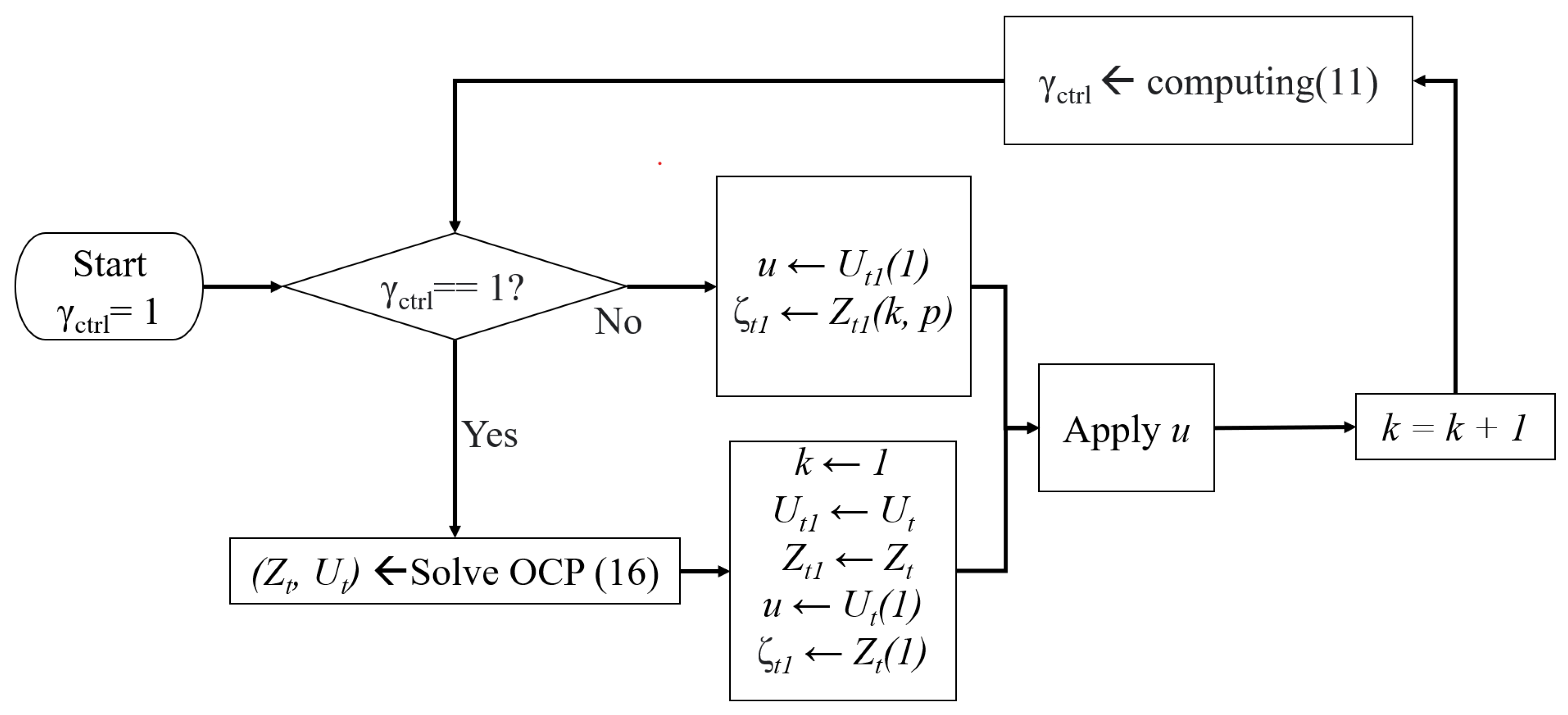
Algorithm 1 Event-triggered MPC [46]

1: procedure eMPC($\widehat{\zeta }$, k, $U_{t_1}$, $Z_{t_1}$, p)  2:     $k\leftarrow k+1$;  3:     ${\gamma }_{ctrl}\leftarrow$ Computing (11);  4:     if ${\gamma }_{ctrl}=1$ then  5:         $k\leftarrow 1$;  6:         $(Z_t,U_t)\leftarrow$ Solving OCP (16);  7:         $u\leftarrow U_t\left(1\right)$;  8:         $\zeta \leftarrow Z_{t_1}\left(1\right)$;  9:         $U_{t_1}\leftarrow U_t$; 10:         $Z_{t_1}\leftarrow Z_t$; 11:     else 12:         $u\leftarrow U_{t_1}\left(1\right)$; 13:         if $k<=p$ then 14:            $\zeta \leftarrow Z_{t_1}\left(k\right)$ 15:         else 16:            $\zeta \leftarrow Z_{t_1}\left(p\right)$ 17:         end if 18:     end if 19:     return u, $\zeta$, $U_{t_1}$, $Z_{t_1}$, k 20: end procedure

3. Problem Formulation

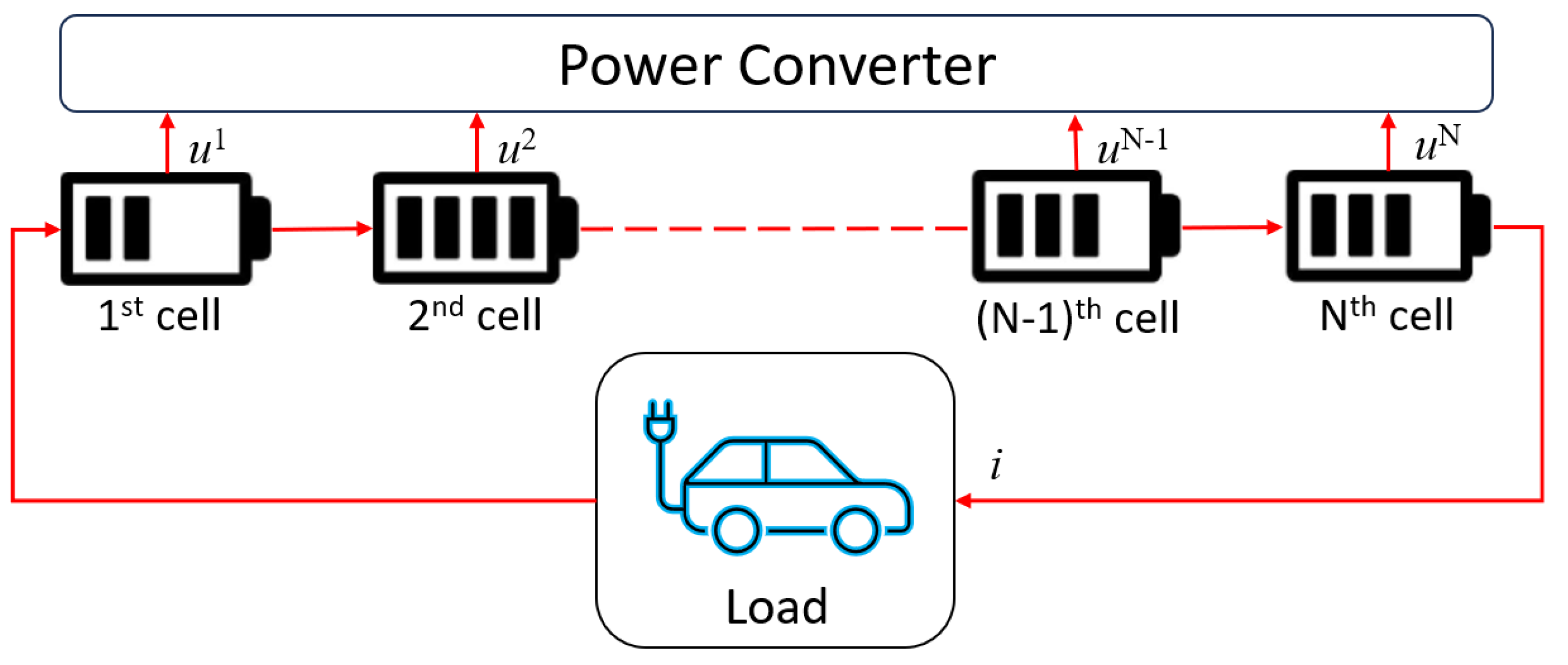
3.1. Active-Battery-Cell-Balancing Control

A common equivalent circuit model of a lithium-ion cell can be used to model the SOC, relaxation voltage, and terminal voltage of each cell [47,48]. The cell model can be described as

$$\begin{array}{}\mathrm{(12a)}& \hfill {\dot{s}}^n& =-{\eta }^n\frac{i^n}{C^n}\hfill \mathrm{(12b)}& \hfill {\dot{V}}_p^n& =-\frac{V_p^n}{R_p^n{C}_p^n}+\frac{i^n}{C_p^n}\hfill \mathrm{(12c)}& \hfill y^n& =V_{oc}^n-V_p^n-i^n{R}_o^n,\hfill \end{array}$$

where the superscript n indicates the nth cell, $s^n$ is the cell SOC, ${\eta }^n$ is the cell Coulombic efficiency, $C^n$ is the cell capacity in amp hours, $V_p^n$ is the relaxation voltage over $R_p^n$, $V_{oc}^n$ is the open-circuit voltage, $y^n$ is the terminal voltage, and $i^n$ is the cell current. Positive $i^n$ indicates discharging the battery, while negative $i^n$ indicates charging. The variables $V_{oc}^n$, $R_o^n$, $R_p^n$, and $C_p^n$ are all dependent on $s^n$, resulting in a nonlinear cell model.

This model can then be discretized using Euler’s method for a model that can be implemented digitally as

$$\begin{array}{}\mathrm{(13a)}& \hfill s_{k+1}^n& =s_k^n-{\eta }^n\frac{T_s}{C^n}{i}_k^n\hfill \mathrm{(13b)}& \hfill V_{p,k+1}^n& =V_{p,k}^n-\frac{T_s}{R_p^n{C}_p^n}{V}_{p,k}^n+\frac{T_s}{C_p^n}{i}_k^n\hfill \mathrm{(13c)}& \hfill y_k^n& =V_{oc,k}^n-V_{p,k}^n-i_k^n{R}_o^n,\hfill \end{array}$$

where $T_s$ was set to 1 s. To simulate an imbalance, a probability distribution can be used to apply random variation to the $C^n$, $R_o^n$, and $C_p^n$ terms.

Table 1. Cell imbalance parameters at 100% SOC. Ah: amp-hour; mΩ: milliohms; kF: kilofarads.

Parameter	Unit	$\mathit{n}=1$	$\mathit{n}=2$	$\mathit{n}=3$	$\mathit{n}=4$	$\mathit{n}=5$
C	Ah	62.87	60.00	66.61	56.73	61.66
$R_p$	mΩ	6.40	5.66	5.47	6.68	6.36
$C_p$	kF	153.7	177.8	175.9	168.9	150.4
$R_o$	mΩ	1.49	1.27	1.41	1.51	1.53

lists example variations in these parameters that were later used for the simulation in this paper.

Finally, the SOC and relaxation voltage states can be grouped together as ${\zeta }^n:={[s^n,V_p]}^T$, where ${.}^T$ denotes a matrix or vector transpose. The battery pack state can be written as

$$\begin{array}{}\mathrm{(14a)}& \hfill {\zeta }_{k+1}^n& =f^n({\zeta }_k^n,i_k+u_k^n)\hfill \mathrm{(14b)}& \hfill y_k^n& =g^n({\zeta }_k^n,i_k+u_k^n),\hfill \end{array}$$

where $u_k^n$ is the balancing current applied to the cell, as shown in Figure 2. Defining $\zeta ={[{\zeta }^1,{\zeta }^2,\dots ,{\zeta }^N]}^T$ as the state vector for the battery pack and y as the terminal voltage of the battery pack, then

$$\begin{array}{}\mathrm{(15a)}& \hfill {\zeta }_{k+1}& =\left[\begin{array}{c}{f}^n({\zeta }_k^1,i_k+u_k^1)\\ f^n({\zeta }_k^2,i_k+u_k^2)\\ ⋮\\ f^n({\zeta }_k^N,i_k+u_k^N)\end{array}\right]\hfill \mathrm{(15b)}& \hfill y_k& =\sum _{m=1}^N{y}_k^n=\sum _{m=1}^N{g}^n({\zeta }_k^n,i_k+u_k^n).\hfill \end{array}$$

For this study, a pack with 5 cells in series is assumed, resulting in a pack terminal voltage equal to the sum of the cell terminal voltages. For the active-cell-balancing power converter, an ideal converter with limits on each balancing current and no charge storage is assumed. This power converter also assumes a direct cell–cell topology, meaning that charge from any cell can be directed to any other cell, with the rate of charge transfer limited by balancing current limits. These constraints, along with the cell model, can be formulated as an optimal control problem for MPC at time step k over prediction horizon p as

$$\begin{array}{}\mathrm{(16a)}& \hfill \underset{Z_t,U_t}{min}& \sum _{k=1}^p{J}_{mpc}^k(Z_t,U_t)\hfill & \hfill \mathrm{s}.\mathrm{t}.& {\zeta }_{k+j+1}^n=f^n({\zeta }_{k+j}^n,i_{k+j}+u_{k+j}^n),\hfill \mathrm{(16b)}& & 0\le j\le p-1,1\le n\le N\hfill & \hfill & y_{k+j}^n=g^n({\zeta }_{k+j}^n,i_{k+j}+u_{k+j}^n),\hfill \mathrm{(16c)}& & 1\le j\le p,1\le n\le N\hfill \mathrm{(16d)}& \hfill & u_{min}\le u_k^n\le u_{max},1\le n\le N\hfill \mathrm{(16e)}& \hfill & \underline{y}\le y_{k+j}^n,1\le j\le p,1\le n\le N\hfill \mathrm{(16f)}& \hfill & 0=\sum _{i=1}^N{u}_k^n.\hfill \end{array}$$

The constraints on the optimization problem begin with (16d) to set maximum and minimum limits for each balancing current $u_n^k$. Next, (16e) states that the cell terminal voltages $y_{k+j}^n$ must be greater than the DVL $\underline{y}$. Finally, (16f) states that there is no charge storage, only transfer, with the sum of balancing currents equal to 0.

The cost function chosen for this study is based on minimizing the tracking error between each individual cell to a nominal cell without an imbalance, which was studied in [1]. This MPC formulation can be presented mathematically as

$$J_y\left(u_k\right)=\sum _{j=1}^p{(y_{k+j}-y_{k+1}^0)}^T(y_{k+j}-y_{k+1}^0)+u_k^{T}R{u}_k,$$

(17)

where $y_{k+j}$ is defined as the vector of cell terminal voltages $y_{k+j}={[y_{k+j}^1,y_{k+j}^2,\cdots y_{k+j}^N]}^T$, and R is a positive semi-definitive weighting matrix. The first term penalizes cell voltages that deviate from the nominal cell, while the second term penalizes the magnitude of the balancing current to reduce resistant heating losses. The nominal cell voltage target is a scalar, which means that only the R weighting matrix is needed to tune the cost of the terms.

3.2. RLeMPC for Active Cell Balancing

The MPC controller that solves (16) periodically is then adapted to eMPC by first integrating an event trigger into the MPC model using the difference between the predicted voltage of a nominal cell and the measured terminal voltage of each cell compared to a calibratable threshold $\overline{e}$ as the trigger condition described in (11). When the event is not triggered (${\gamma }_{ctrl}=0$), the controller holds the first of the balancing commands of the previous calculated series $U_{t_1}$ instead of using the subsequent elements of $U_{t_1}$. This modification was used because the future driver power demand is assumed to be unknown, and the dynamics of the terminal voltage are relatively slow compared to the controller sample rate of $T_s=1$ s. This implementation of eMPC was studied to compare to a constant time-triggered MPC baseline and an RL-based event trigger.

After testing and evaluating the eMPC implementation, an RL agent was developed to replace the trigger conditions. The RL agent was set up as a DQN agent, described above in Section 2.2. This agent interacts with the environment (15) and observes the average and minimum cell voltages, the average cell SOC, and the pack current demand as state variables as well as the reward (18). Although each cell voltage is considered in the state in (15), only these more general state parameters were used to reduce the number of dimensions of the state for training. During training, the agent will select a random action with a probability $ϵ$ that decays exponentially over time, and otherwise, it will select the action with the greatest value determined by the critic network with parameters $\varphi$. This action is the event-trigger for the MPC controller to solve the OCP, which then determines a new $U_{t_1}$ and $Z_{t_1}$. The reward function for each time step was defined as the distance driven over the time step $dx$ subtracted by a flag representing whether or not the event trigger was set, ${\gamma }_{ctrl}$, multiplied by a weighting factor $\rho$, together defined as

$$r=dx-{\gamma }_{ctrl}\times \rho .$$

(18)

This reward function is one of the primary design elements for the RLeMPC implementation, where the key objectives of maximizing the EV range in $dx$ and minimizing event triggering in ${\gamma }_{ctrl}$ are included for the agent to pursue. This reward r is the main feedback signal that the RL agent uses to learn an optimal policy that maximizes r over the episode. The parameter $\rho$ was tuned to achieve the proper scaling between the conflicting objectives to result in the desired behavior of the converged policy. With these RL state and reward formulations, many hyperparameters, such as $\rho$, the structure of the DQN, the learning rate, the discount factor, and epsilon decay, were tuned in a simulation environment while training the agent to find the optimal event-trigger policy. The details for training the RLeMPC agent can be found in Algorithm 2 and Figure 3.

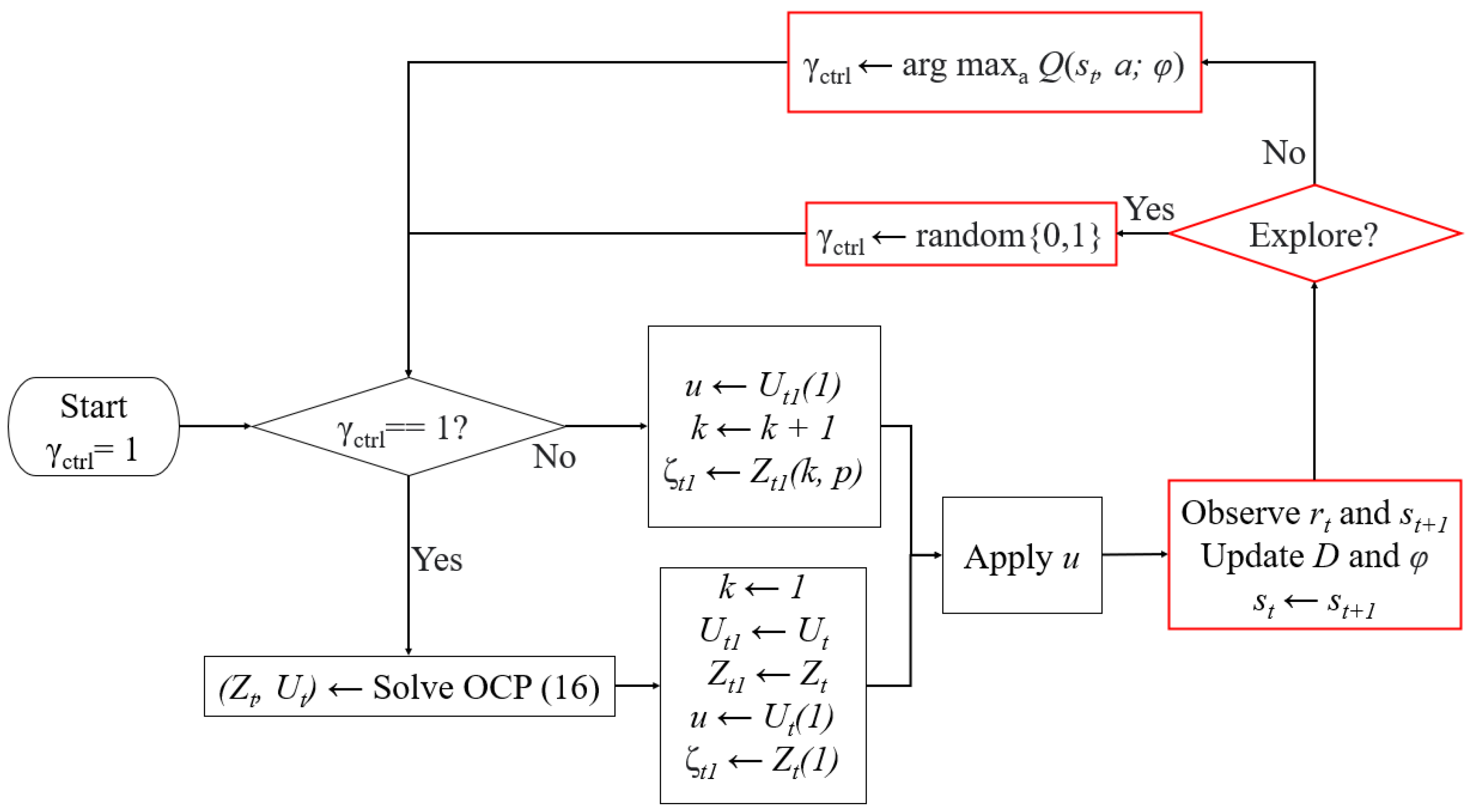
Algorithm 2 RL-based event-triggered MPC

1: procedure RLeMPC(M, T, $dt$, $\gamma$, N)  2:     Initialize $\varphi$, $\mathcal{D}\leftarrow \varnothing$, ${\varphi }_t\leftarrow \varphi$  3:     for $j=0$ to $N-1$ do  4:         Initialize $s_t$, $Z_{t_1}$, $U_{t_1}$, $k\leftarrow 0$, $u\leftarrow 0$  5:         while $t<=T$ do  6:            if explore then  7:                Sample $a_t$ from $\{0,1\}$  8:            else  9:                $a_t\leftarrow {arg\; max}_{a}Q(s_t,a;\varphi )$ 10:            end if 11:            <Simulate Environment> 12:            if ${\gamma }_{ctrl}=1$ then 13:                $k\leftarrow 0$; 14:                $(Z_t,U_t)\leftarrow$ Solving OCP (16); 15:                $u\leftarrow U_t\left(1\right)$; 16:                $U_{t_1}\leftarrow U_t$; 17:                $Z_{t_1}\leftarrow Z_t$; 18:            else 19:                $u\leftarrow U_{t_1}\left(1\right)$; 20:                $k\leftarrow k+1$; 21:                if $k<=p$ then 22:                    $\widehat{\zeta }\leftarrow Z_{t_1}\left(k\right)$ 23:                else 24:                    $\widehat{\zeta }\leftarrow Z_{t_1}\left(p\right)$ 25:                end if 26:            end if 27:            ${\zeta }_{t+1}\leftarrow$ Simulate (13) using u 28:            $s_{t+1}\leftarrow {\zeta }_{t+1}$ 29:            $r_t\leftarrow \left(18\right)$ 30:            <End of Environment Simulation> 31:            Observe $r_t$ and $s_{t+1}$ 32:            Update $\mathcal{D}$ to include $(s_t,a_t,r_t,s_{t+1})$ 33:            Sample M experiences from $\mathcal{D}$ 34:            $\varphi \leftarrow$ Perform gradient descent on (6) 35:            if Target Update Condition is True then 36:                ${\varphi }_t\leftarrow \varphi$ 37:            end if 38:            $s_t\leftarrow s_{t+1}$ 39:            $t\leftarrow t+dt$ 40:         end while 41:     end for 42: end procedure

4. Simulation Results and Discussion

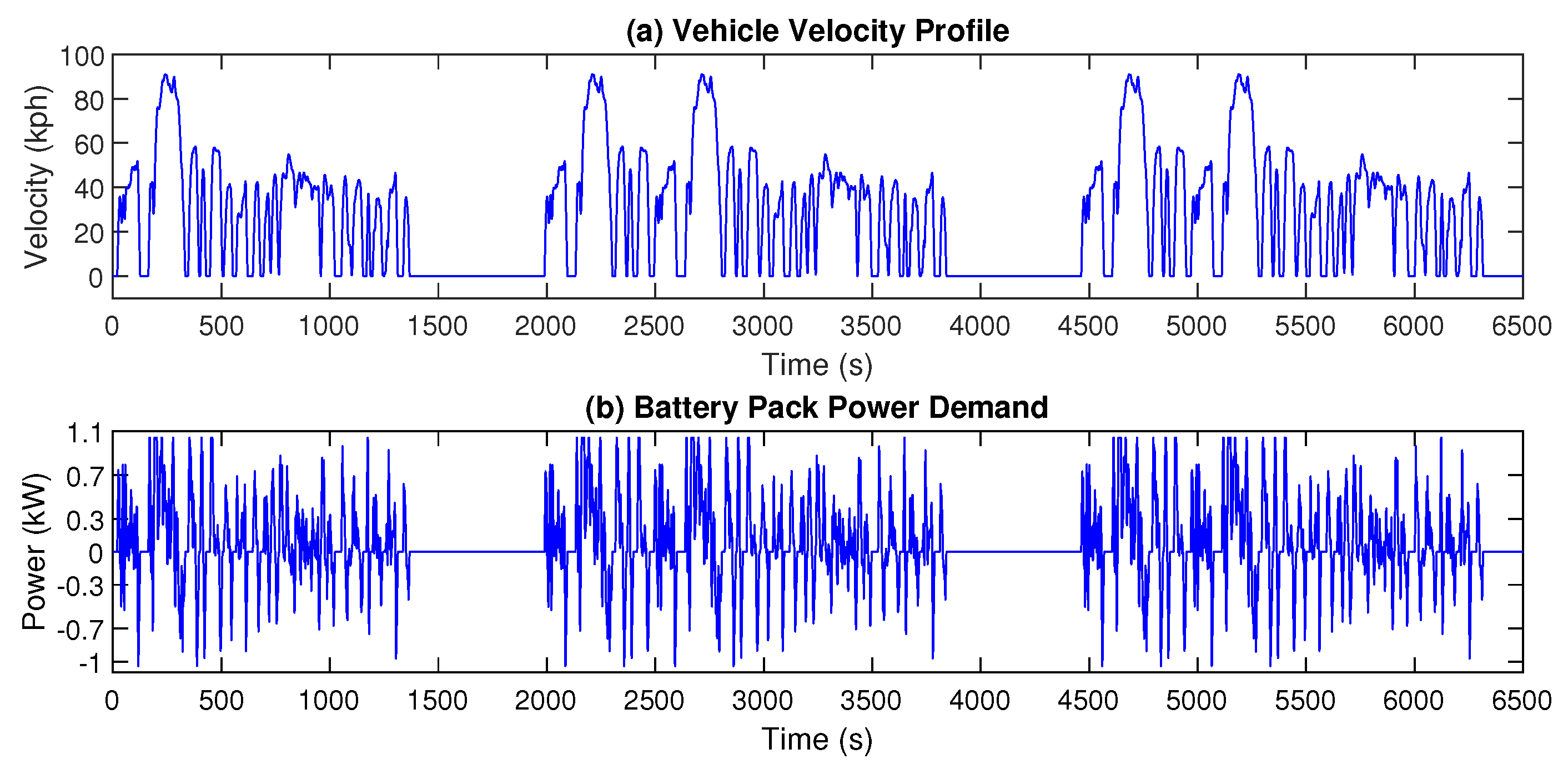
4.1. Simulation Environment

Simulations were executed for the training and testing of the active-cell-balancing controls using MATLAB and Simulink (R2021a) with the Reinforcement Learning Toolbox to create and train DQN agents inside of a Simulink environment [49]. The simulations were conducted on a computer with an Intel^® Core^TM i5-6600K processor and 8 GB of RAM. As described above, the system being simulated is a battery pack with five cells in series and an ideal power converter that can move charge between any cells, constrained by a balancing current limit of ±2 A for each cell.

Repeated FTP-72 drive cycle conditions were tested over the sedan EV configuration used in [1]. The discharge current from the battery pack was scaled from the power demand to assume a larger pack with additional modules in parallel, and a final scaling factor was applied to increase the current draw and reduce the simulation time. Starting with all cells fully charged to the CVL, the battery was discharged according to the scaled current demand of the vehicle until the first cell reached the DVL. The velocity profile and scaled vehicle power demand that were applied to the 5S cell module are shown in Figure 4, where, in subsequent cycles, phase 1 of the cycle is repeated for the higher power demands to discharge the battery faster.

Finally, for all the simulations, a constant imbalance was applied across the $C^n$, $R_o^n$, $C_p^n$, and $R_p^n$ cell parameters. To select these parameters, a series of simulations were run that multiplied each of the nominal cell parameters by random factors, which were selected from a normal distribution with a mean of 1 and an interval between 0.9 and 1.1. From these tests, a set of imbalance factors that resulted in an average active-cell-balancing range extension benefit for the configuration with the conventional MPC approach was chosen as the constant set of imbalance parameters to use for the rest of the simulations. This was carried out because the magnitude of the imbalance determines the range extension benefit that can be realized with active cell balancing. With less of a realizable range extension benefit, the sensitivity of the range extension, depending on the control strategy, is reduced as it changes between MPC, eMPC, and RLeMPC. Future work could include how to generalize these approaches to any distribution of imbalances and quantify the benefit relative to the distribution of cell imbalances, especially for the RL agent, which was trained and evaluated using only one set of imbalance parameters in this study.

4.2. Evaluation Criteria

The primary performance metrics for this study are the overall driving range and average event-trigger frequency. The purpose of cell balancing in general is to achieve the maximum energy output of the battery, which would translate to maximizing the driving range, assuming no auxiliary loads. Moreover, the average execution frequency is used as an approximation of the computational load, with the goal of minimizing it with RLeMPC. In addition, the magnitude of the balancing currents averaged over the drive cycle is considered to approximate the resistant heating losses and referred to as the balancing effort in the sequel.

4.3. Results with Constant Trigger Period

Before executing simulations with varying trigger frequencies, the MPC weighting matrix R in (17) was re-calibrated to be more robust to infrequent triggering. For conventional MPC or eMPC with minimal modeling errors, the weighting of R can be decreased to tune the cost optimization toward lower voltage tracking errors of the cells to a nominal cell voltage target at the cost of higher balancing currents. However, for this application, where the future driver power demand is assumed to be unknown, weighting to prioritize aggressively tracking the reference voltage can result in a reduced range extension. The unknown future driver power demand becomes a disturbance in the model prediction, which increases as the trigger frequency is reduced. Furthermore, the prediction horizon may occasionally be much less than the trigger period, resulting in a prediction error even if the power demand was known ahead of time. Because of these unknown dynamics in the model, increasing the cost of the balancing current magnitude through the weighting matrix R can increase the range performance of the system during infrequent triggering by reducing the response of the controller to a model with large prediction errors.

This dynamic is shown in Figure 5, where the cost weighting of each balancing current magnitude $R^n$ is set to be equal, scaled appropriately, and tested to determine range extension and balancing effort dependencies. For these tests, the value of $R^n$ was varied for transient cycle discharge tests while having a constant trigger period of 5 s. Increasing the $R^n$ values leads to less balancing effort, which demonstrates the effect of R on the MPC cost optimization. For $R^n$ in 800–4000, the range is extended by 0.1% as compared to when $R^n$ is between 10 and 70. Although a small difference, this result demonstrates that, with these model assumptions, larger $R^n$ values can result in a larger range extension. This result may not be intuitive since a range extension is gained with less balancing effort, but this comes from the previously described modeling discrepancies. Once R is very large, the range extension decreases drastically as the balancing currents are greatly reduced, limiting the optimal calibration range for $R^n$. The final $R^n$ calibration was set to 100 to avoid the initial large amounts of balancing effort and also to avoid overly penalizing the balancing effort. Figure 6 shows the transient cell-balancing performance for the final R calibration and a constant trigger period of 5 s.

Once the weighting matrix was calibrated, the first study that was completed was for a varying constant trigger frequency. These tests were simulated to understand, as a baseline without any event triggers, the range extension and balancing current magnitudes when only varying the trigger frequency of the MPC controller. For this purpose, the trigger frequency was set to a constant value starting from 1 Hz and decreased between simulations until 0 triggers occurred. This trigger frequency range demonstrates the maximum and minimum driving ranges achievable. For these tests, the prediction horizon remained 5 s, with only the first element of the control sequence $U_t$ being applied until another trigger occurred. Notably, the time period between triggers can be greater than the prediction horizon, as described in Section 3.2.

The transient cycle range extension results plotted in Figure 7 indicate that the maximum range of 48.66–48.67 km can be achieved with a constant trigger period of 1 to 700 s or a frequency of 1Hz to 1 mHz, with the balancing effort varying as the trigger period changes. Noticeably, two discrete ranges emerge, with the higher-trigger-frequency tests from 1 Hz down to 1 mHz resulting in approximately this maximum range and tests with frequencies below 1 mHz ending at around a minimum range of 46.23–46.24 km. Figure 8 shows effective cell balancing with a constant trigger period of 1000 s and can be compared to Figure 6 to notice the much less busy balancing current, which delivered nearly the same final driving distance. The discrete driving range levels are attributable to the current scaling that was applied to the transient cycle simulations, which leads to these discrete windows emerging for when the DVL is reached.

To expand on this, Figure 9 shows the vehicle velocity profile along with the transient pack current demand and minimum cell voltage for a simulation that did not reach the DVL during the time window in which other simulations with poor cell balancing did reach the DVL. This occurs in the third repeated cycle, where the DVL is reached at a pack SOC of 33% and a current demand of 280–380 A. The simulations with higher trigger frequencies continued for a fourth cycle until the DVL was reached at a pack SOC of 29% and close to a 400 A cell current demand. Cell terminal voltages decreased significantly during these high-current discharges due to the large internal resistance of the cell. This current scaling, along with the nonlinear OCV, creates these discrete final driving ranges such that the first current peak where the DVL is reached may be overcome by cell balancing, but the second current peak, where the rest of the simulations reach the DVL, cannot be overcome. The second current peak cannot be overcome even with perfectly balanced cells and a significant 29% SOC remaining because of the large current demands. This effect could be smoothed out with more realistic cell currents at the cost of a longer simulation time. However for this study, especially when testing RLeMPC, the simulation times had to be short to train the RL agent in a reasonable amount of time. These results are sufficient for the initial concept demonstration to test whether RLeMPC can determine the optimal eMPC trigger policy to overcome the first high-power window.

4.4. Results with Threshold-Based eMPC

For eMPC, simulations with varying error thresholds were executed to understand whether an eMPC approach could outperform the constant-trigger-frequency MPC controller in terms of the range extension, average trigger frequency, and balancing effort. Figure 10 shows that as the error threshold increased, the trigger frequency decreased approximately exponentially until saturating at 0–1 trigger per test. Between error thresholds of 1 and 1.5 V, the exponential relationship begins to break as the cell balancing fails to avoid the DVL during the first very-high-current peak, as illustrated in the large step of the driving range around 10 mHz in Figure 11. Compared to the constant-trigger-frequency results, eMPC did not achieve as much of a range extension as MPC at reduced average triggering frequencies. For example, most of the frequency range between 10 mHz and 1 mHz reached the DVL at a driving range of 46.24 km for eMPC, while for constant-trigger-frequency MPC in this frequency range, the DVL was reached at 48.66 km. Additionally, the average balancing effort is higher on average and more variable for eMPC. Overall, constant-trigger-frequency MPC performs better than eMPC according to the evaluation criteria for this application and this trigger condition, highlighting the challenge of implementing an optimal eMPC trigger condition.

The transient results for eMPC with the lowest average event-trigger frequency that achieved 48.66 km are plotted in Figure 12. In this example, the benefit of eMPC is demonstrated by the lack of event triggers during the standstill portions between repeated cycles when triggering is not required. This control strategy can be effective when the load is 0 or constant, but during the transient portions of the test, the actual cell voltages are much more transient relative to the nominal voltage target computed when the OCP is solved, causing excessive triggering. Changing the target voltage to the average actual cell voltage instead of a nominal predicted cell target may be an improvement in the event-trigger policy to account for modeling errors arising from the unpredictable driver power request.

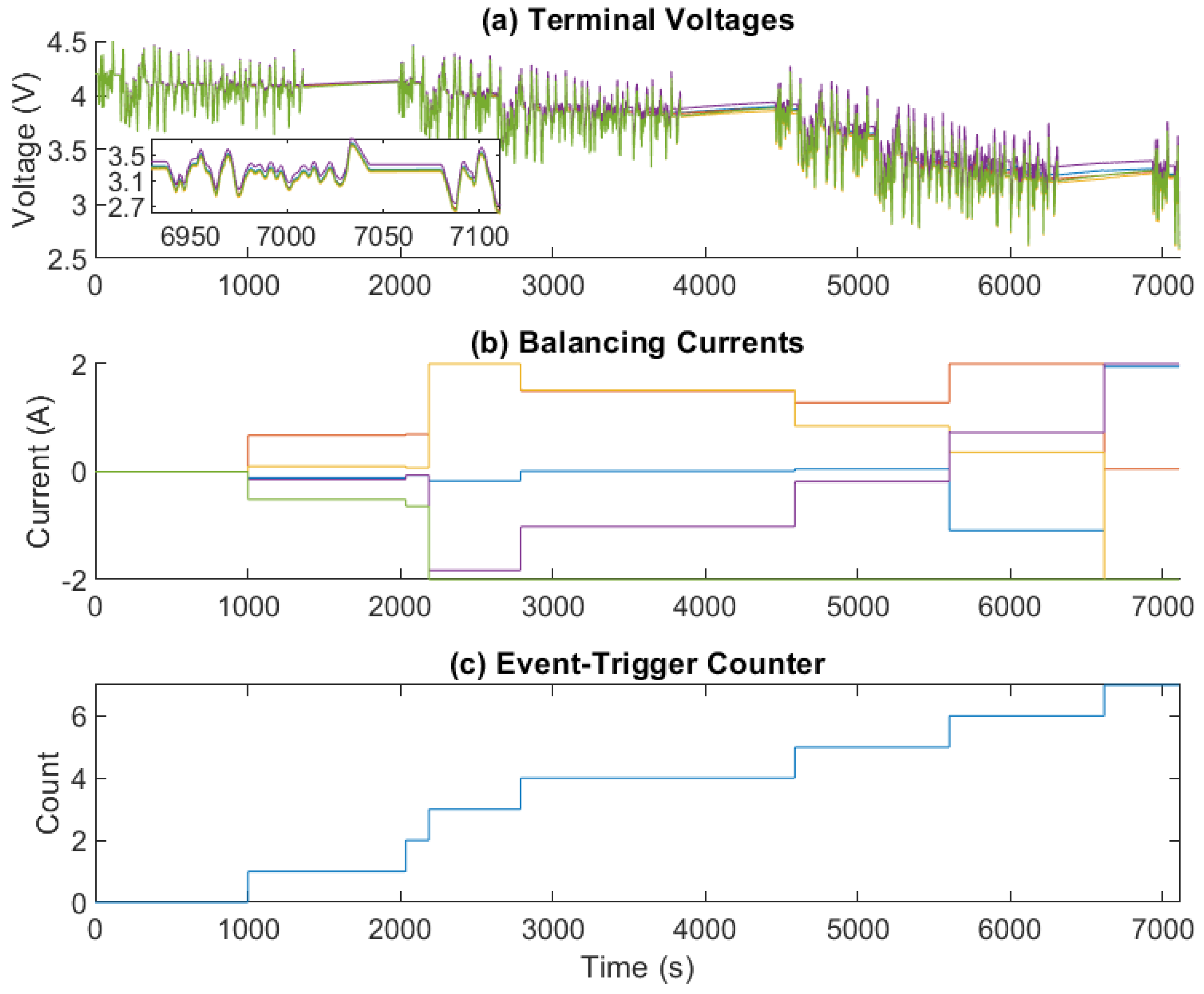
4.5. Results with RLeMPC

Many challenges were encountered while training the RLeMPC agent. For this problem, only a minimal number of triggers is required to achieve the maximum reward, and any number of triggers below the minimum results in very little range extension benefit. This feature of the dynamics leads to the RL agent learning a sub-optimal policy of triggering very infrequently, or the training can diverge to triggering excessively. Because of the penalty for triggering in the reward function, the RL agent can learn a policy of not triggering at all, which would be the optimal policy if the first current peak could not be overcome with cell balancing. Depending on how the RL agent is trained, the agent can erroneously learn this as the optimal policy even after having experienced the larger driving ranges that are achievable. While training the agent, this local optimum became very difficult to avoid, even with a low weighting factor $\rho$ applied to the trigger action in the reward function.

Two important training parameters that were explored to avoid this local optimum were the discount factor $\gamma$ and the $ϵ$-decay exploration method. To start with $\gamma$, typical values like 0.9 and 0.99 overly discounted the future delayed range extension reward from cell balancing thousands of steps in advance. To account for these delayed rewards, $\gamma$ in the range of 0.999–0.9999 was required, but such a high value for $\gamma$ required more training to accurately learn which actions lead to delayed rewards. Extended training time or a more refined approach to addressing the delayed rewards in this problem may be required to learn the optimal policy. This feature differentiates the active-cell-balancing problem from other problems with less delayed rewards, such as autonomous vehicle path following, for which RLeMPC was successfully applied in [18].

The $ϵ$-decay method for training was another major challenge for this problem. Typically, $ϵ$ was initialized at around 1 and decayed to a minimum value to explore the environment before transitioning to exploiting the environment to maximize G. For this problem, the maximum final range can be achieved with very little triggering, so with high $ϵ$ and a 50% probability of choosing to trigger for a random action, the agent first learned the penalty from triggering because it always achieved the maximum range at the beginning of the training. As $ϵ$ decayed, the agent transitioned from random actions to following actions with greater learned Q-values from the DQN, which initially meant no triggers at all. Eventually, $ϵ$ decayed enough to where not enough triggering occurred from random actions to achieve the maximum range, and during this transition, it was very difficult for the agent to learn that triggering more could lead to a much greater range extension. Part of this could come from the fact that the agent could not learn the distinction in the driving range extension between triggering and not triggering at the beginning of the training. Next, once it did not trigger enough to overcome the first high-current peak, it could not learn quickly enough that triggering could lead to a larger range extension reward before falling into the local optimum of not triggering at all with no driving range extension.

This example of training plays out in Figure 13a, where the reward correlates with $ϵ$ from the decrease in the trigger frequency until around 400 episodes, after which triggering was not frequent enough to overcome the first high-current peak. The switching observed in the episode reward was from going between the high and low final driving ranges with large reward weighting applied to the driving range extension. After this transition, the RL agent settled into a policy of not triggering at all to maximize the reward with no driving range extension.

To attempt to overcome this challenge of learning a sub-optimal policy during the exploration phase of the training, $ϵ$ was initialized to much lower values for training. These values were chosen from the maximum episode length of around 7000 steps with only two actions available per step, which still results in a significant number of exploratory actions. The MPC and eMPC results show that around 100–1000 s per trigger or 7–70 triggers per episode is the minimum number of triggers required to achieve a large driving range extension. This new $ϵ$-decay tuning, along with random initial weights and biases for the DQN, was chosen to try to initialize the training right at the step of the low-to-high driving range extension so that the agent experiences the range extension difference between triggering and not triggering right away.

Attempts at this $ϵ$-decay tuning did not improve the training performance. First, when $ϵ$ is not low enough, the agent learns to not trigger, falling into the local optimum of 0 triggers per episode, as shown in Figure 13b,c. For these training sets, $ϵ$ was initialized to 40% and 5%, and both resulted in the same policy of not triggering to maximize the reward when no driving range extension is achieved. From these training sets, an $ϵ$ of 1–5% appears to be the best value to begin the training since this is the range where the switching between high and low driving distance ranges begins to be observed. However, initializing $ϵ$ to 1%, as shown in Figure 13d, resulted in the training diverging and the reward decreasing; the maximum distance was always achieved, but the RL agent learned to trigger more.

The next steps that are planned for improving upon the results presented include the focused tuning of $\gamma$, $ϵ$-decay, and the reward weighting $\rho$ around the driving range transition trigger frequencies. The expectation is that the data efficiency of the training can be increased by a focused exploration in the key trigger frequency range. The first step is to find a proper initial value of $ϵ$, as well as a more effective $ϵ$-decay rate. As mentioned, an initial $ϵ$ value of 1–5% should be appropriate to place the initial trigger frequency around where the step of the driving range occurs, but slowing down the $ϵ$-decay rate may help give the agent more time to explore in the key $ϵ$ range. Additionally, varying the initial DQN weights and reward weighting may help to avoid the diverging behavior observed in Figure 13d. Finally, tuning $\gamma$ in this more effective exploration range should be beneficial to ensuring that delayed rewards are weighted properly to attribute the range extension benefit to the earlier triggering.

Overall, the analysis from tuning this DQN agent for active cell balancing can provide guidance for tuning $\gamma$, $ϵ$-decay, and the reward function for a particular problem when training for tens of thousands of episodes is not a viable option. The above next steps identified will be included in future work to report on their effectiveness in improving the performance of training the RL agent. One glimmer of the potential comes from the switching observed in rewards at low $ϵ$ values in Figure 13. The high values in that switching represent episodes where the RL agent achieved a larger range extension with very little triggering from random actions. For example, Figure 14 shows the cell balancing and triggering occurring during one of those episodes, where only seven random triggers resulted in a final driving range of 48.66 km. This performance is on par with the constant, infrequent MPC triggering approach, showing that improvement is possible if the RL agent can be trained to learn it. Finally, adjusting the current scaling of the simulation may also help shape the Q-function to be more variable, easier to learn, and more reflective of the actual-cell-balancing problem.

5. Conclusions

Three model predictive control (MPC) strategies, namely, time-triggered MPC, event-triggered MPC (eMPC), and reinforcement learning-based MPC (RLeMPC), for active cell balancing were formulated and tested in a simulation environment to reduce the computational requirements relative to a baseline MPC controller while maintaining the EV range extension benefit. MPC with reduced constant periodic triggering and eMPC control methods demonstrated a significant computational load reduction with average trigger period increases to 1000 s and 187 s, respectively, compared to the 1 s trigger period of baseline MPC. Only a negligible decrease in the EV range extension of 0.03% from the maximum achievable range was the penalty for this significant decrease in throughput. By scaling the current demand for a more efficient simulation, the discharge voltage limit was reached at very high cell current demands, between 280 and 380 A, with 33% state of charge remaining in the battery pack, shaping the EV range extension results. The challenges of training the RLeMPC agent were presented, such as the discrete and delayed range extension rewards, as well as an ineffective exploration method. Overall, the converged RLeMPC policy was very sensitive to training, which will be further improved by hyperparameter tuning, but occasional training episodes were promising with a greater than 1000 s average trigger period. Future steps to address these challenges, to learn more optimal event-trigger policies, and to improve the robustness of the proposed approach were discussed and are planned as future work. Real-world implementation in a microcontroller is another future work direction.

References

1. Chen, J.; Behal, A.; Li, C. Active battery cell balancing by real time model predictive control for extending electric vehicle driving range. IEEE Trans. Autom. Sci. Eng. 2023; accepted. [Google Scholar] [CrossRef]
2. Preindl, M. A battery balancing auxiliary power module with predictive control for electrified transportation. IEEE Trans. Ind. Electron. 2017, 65, 6552–6559. [Google Scholar] [CrossRef]
3. Liu, J.; Chen, Y.; Fathy, H.K. Nonlinear model-predictive optimal control of an active cell-to-cell lithiumion battery pack balancing circuit. IFAC PapersOnLine 2017, 50, 14483–14488. [Google Scholar] [CrossRef]
4. Razmjooei, H.; Palli, G.; Abdi, E.; Terzo, M.; Strano, S. Design and experimental validation of an adaptive fast-finite-time observer on uncertain electro-hydraulic systems. Control. Eng. Pract. 2023, 131, 105391. [Google Scholar] [CrossRef]
5. Shibata, K.; Jimbo, T.; Matsubara, T. Deep reinforcement learning of event-triggered communication and consensus-based control for distributed cooperative transport. Robot. Auton. Syst. 2023, 159, 104307. [Google Scholar] [CrossRef]
6. Abbasimoshaei, A.; Chinnakkonda Ravi, A.; Kern, T. Development of a new control system for a rehabilitation robot using electrical impedance tomography and artificial intelligence. Biomimetics 2023, 8, 420. [Google Scholar] [CrossRef]
7. Zhang, Y.; Huang, Y.; Chen, Z.; Li, G.; Liu, Y. A novel learning-based model predictive control strategy for plug-in hybrid electric vehicle. IEEE Trans. Transp. Electrif. 2021, 8, 23–35. [Google Scholar] [CrossRef]
8. Rostam, M.; Abbasi, A. A framework for identifying the appropriate quantitative indicators to objectively optimize the building energy consumption considering sustainability and resilience aspects. J. Build. Eng. 2021, 44, 102974. [Google Scholar] [CrossRef]
9. Tøndel, P.; Johansen, T.A.; Bemporad, A. An algorithm for multi-parametric quadratic programming and explicit mpc solutions. Automatica 2003, 39, 489–497. [Google Scholar] [CrossRef]
10. Wang, Y.; Boyd, S. Fast model predictive control using online optimization. IEEE Trans. Control Syst. Technol. 2010, 18, 267–278. [Google Scholar] [CrossRef]
11. Badawi, R.; Chen, J. Performance evaluation of event-triggered model predictive control for boost converter. In Proceedings of the 2022 IEEE Vehicle Power and Propulsion Conference, Merced, CA, USA, 1–4 November 2022. [Google Scholar]
12. Li, H.; Shi, Y. Event-triggered robust model predictive control of continuous-time nonlinear systems. Automatica 2014, 50, 1507–1513. [Google Scholar] [CrossRef]
13. Brunner, F.D.; Heemels, W.; Allgöwer, F. Robust event-triggered MPC with guaranteed asymptotic bound and average sampling rate. IEEE Trans. Autom. Control 2017, 62, 5694–5709. [Google Scholar] [CrossRef]
14. Zhou, Z.; Rother, C.; Chen, J. Event-triggered model predictive control for autonomous vehicle path tracking: Validation using CARLA simulator. IEEE Trans. Intell. Veh. 2023, 8, 3547–3555. [Google Scholar] [CrossRef]
15. Yoo, J.; Johansson, K.H. Event-triggered model predictive control with a statistical learning. IEEE Trans. Syst. Man Cybern. Syst. 2021, 51, 2571–2581. [Google Scholar] [CrossRef]
16. Badawi, R.; Chen, J. Enhancing enumeration-based model predictive control for dc-dc boost converter with event-triggered control. In Proceedings of the 2022 European Control Conference, London, UK, 12–15 July 2022. [Google Scholar]
17. Yu, L.; Xia, Y.; Sun, Z. Robust event-triggered model predictive control for constrained linear continuous system. Int. J. Robust Nonlinear Control 2018, 29, 1216–1229. [Google Scholar]
18. Chen, J.; Meng, X.; Li, Z. Reinforcement learning-based event-triggered model predictive control for autonomous vehicle path following. In Proceedings of the American Control Conference, Atlanta, GA, USA, 8–10 June 2022. [Google Scholar]
19. Dang, F.; Chen, D.; Chen, J.; Li, Z. Event-triggered model predictive control with deep reinforcement learning for autonomous driving. IEEE Trans. Intell. Veh. 2023, 9, 459–468. [Google Scholar] [CrossRef]
20. Baumann, D.; Zhu, J.-J.; Martius, G.; Trimpe, S. Deep reinforcement learning for event-triggered control. In Proceedings of the 2018 IEEE Conference on Decision and Control (CDC), Miami, FL, USA, 17–19 December 2018; pp. 943–950. [Google Scholar]
21. Leong, A.S.; Ramaswamy, A.; Quevedo, E.D.; Karl, H.; Shi, L. Deep reinforcement learning for wireless sensor scheduling in cyber–physical systems. Automatica 2020, 113, 108759. [Google Scholar] [CrossRef]
22. Chen, J.; Zhou, Z. Battery cell imbalance and electric vehicles range: Correlation and NMPC-based balancing control. In Proceedings of the 2023 IEEE International Conference on Electro Information Technology, Romeoville, IL, USA, 18–20 May 2023. [Google Scholar]
23. Dubarry, M.; Vuillaume, N.; Liaw, B.Y. Origins and accommodation of cell variations in li-ion battery pack modeling. Int. J. Energy Res. 2010, 34, 216–231. [Google Scholar] [CrossRef]
24. Chen, J.; Zhou, Z.; Zhou, Z.; Wang, X.; Liaw, B. Impact of battery cell imbalance on electric vehicle range. Green Energy Intell. Transp. 2022, 1, 100025. [Google Scholar] [CrossRef]
25. Daowd, M.; Omar, N.; Van Den Bossche, P.; Van Mierlo, J. Passive and active battery balancing comparison based on MATLAB simulation. In Proceedings of the 2011 IEEE Vehicle Power And Propulsion Conference, Chicago, IL, USA, 6–9 September 2011; pp. 1–7. [Google Scholar]
26. Karnehm, D.; Bliemetsrieder, W.; Pohlmann, S.; Neve, A. Controlling Algorithm of Reconfigurable Battery for State of Charge Balancing using Amortized Q-Learning. Preprints 2024. [Google Scholar] [CrossRef]
27. Hoekstra, F.S.J.; Bergveld, H.J.; Donkers, M. Range maximisation of electric vehicles through active cell balancing using reachability analysis. In Proceedings of the 2019 American Control Conference (ACC), Philadelphia, PA, USA, 10–12 July 2019; pp. 1567–1572. [Google Scholar]
28. Shang, Y.; Cui, N.; Zhang, C. An optimized any-cell-to-any-cell equalizer based on coupled half-bridge converters for series-connected battery strings. IEEE Trans. Power Electron. 2018, 34, 8831–8841. [Google Scholar] [CrossRef]
29. Wang, L.Y.; Wang, C.; Yin, G.; Lin, F.; Polis, M.P.; Zhang, C.; Jiang, J. Balanced control strategies for interconnected heterogeneous battery systems. IEEE Trans. Sustain. Energy 2015, 7, 189–199. [Google Scholar] [CrossRef]
30. Evzelman, M.; Rehman, M.M.U.; Hathaway, K.; Zane, R.; Costinett, D.; Maksimovic, D. Active balancing system for electric vehicles with incorporated low-voltage bus. IEEE Trans. Power Electron. 2015, 31, 7887–7895. [Google Scholar] [CrossRef]
31. Xu, J.; Cao, B.; Li, S.; Wang, B.; Ning, B. A hybrid criterion based balancing strategy for battery energy storage systems. Energy Procedia 2016, 103, 225–230. [Google Scholar] [CrossRef]
32. Gao, Z.; Chin, C.; Toh, W.; Chiew, J.; Jia, J. State-of-charge estimation and active cell pack balancing design of lithium battery power system for smart electric vehicle. J. Adv. Transp. 2017, 2017, 6510747. [Google Scholar] [CrossRef]
33. Narayanaswamy, S.; Park, S.; Steinhorst, S.; Chakraborty, S. Multi-pattern active cell balancing architecture and equalization strategy for battery packs. In Proceedings of the International Symposium on Low Power Electronics and Design, Seattle, WA, USA, 23–25 July 2018; pp. 1–6. [Google Scholar]
34. Kauer, M.; Narayanaswamy, S.; Steinhorst, S.; Lukasiewycz, M.; Chakraborty, S. Many-to-many active cell balancing strategy design. In Proceedings of the 20th Asia and South Pacific Design Automation Conference, Chiba, Japan, 19–22 January 2015; pp. 267–272. [Google Scholar]
35. Mestrallet, F.; Kerachev, L.; Crebier, J.; Collet, A. Multiphase interleaved converter for lithium battery active balancing. IEEE Trans. Power Electron. 2013, 29, 2874–2881. [Google Scholar] [CrossRef]
36. Maharjan, L.; Inoue, S.; Akagi, H.; Asakura, J. State-of-charge (SOC)-balancing control of a battery energy storage system based on a cascade PWM converter. IEEE Trans. Power Electron. 2009, 24, 1628–1636. [Google Scholar] [CrossRef]
37. Einhorn, M.; Roessler, W.; Fleig, J. Improved performance of serially connected li-ion batteries with active cell balancing in electric vehicles. IEEE Trans. Veh. Technol. 2011, 60, 2448–2457. [Google Scholar] [CrossRef]
38. Hoekstra, F.S.; Ribelles, L.W.; Bergveld, H.J.; Donkers, M. Real-time range maximisation of electric vehicles through active cell balancing using model-predictive control. In Proceedings of the 2020 American Control Conference, Denver, CO, USA, 1–3 July 2020; pp. 2219–2224. [Google Scholar]
39. Pinto, C.; Barreras, J.; Schaltz, E.; Araujo, R. Evaluation of advanced control for li-ion battery balancing systems using convex optimization. IEEE Trans. Sustain. Energy 2016, 7, 1703–1717. [Google Scholar] [CrossRef]
40. McCurlie, L.; Preindl, M.; Emadi, A. Fast model predictive control for redistributive lithium-ion battery balancing. IEEE Trans. Ind. Electron. 2016, 64, 1350–1357. [Google Scholar] [CrossRef]
41. Altaf, F.; Egardt, B.; Mårdh, L. Load management of modular battery using model predictive control: Thermal and state-of-charge balancing. IEEE Trans. Control. Syst. Technol. 2016, 25, 47–62. [Google Scholar] [CrossRef]
42. Sutton, R.S.; Barto, A.G. Reinforcement Learning: An introduction; MIT Press: Cambridge, MA, USA, 2018. [Google Scholar]
43. Watkins, C.J.C.H. Learning from Delayed Rewards. Ph.D. Thesis, University of Cambridge, Cambridge, UK, 1989. [Google Scholar]
44. Mnih, V.; Kavukcuoglu, K.; Silver, D.; Graves, A.; Antonoglou, I.; Wierstra, D.; Riedmiller, M. Playing atari with deep reinforcement learning. arXiv 2013, arXiv:1312.5602. [Google Scholar]
45. Hasselt, H.V.; Guez, A.; Silver, D. Deep reinforcement learning with double q-learning. In Proceedings of the AAAI Conference on Artificial Intelligence, Phoenix, AZ, USA, 12–17 February 2016; Volume 30. [Google Scholar]
46. Chen, J.; Yi, Z. Comparison of event-triggered model predictive control for autonomous vehicle path tracking. In Proceedings of the IEEE Conference Control Technology and Applications, San Diego, CA, USA, 8–11 August 2021. [Google Scholar]
47. Pei, Z.; Zhao, X.; Yuan, H.; Peng, Z.; Wu, L. An equivalent circuit model for lithium battery of electric vehicle considering self-healing characteristic. J. Control Sci. Eng. 2018, 2018, 5179758. [Google Scholar] [CrossRef]
48. Wehbe, J.; Karami, N. Battery equivalent circuits and brief summary of components value determination of lithium ion: A review. In Proceedings of the 2015 Third International Conference on Technological Advances in Electrical, Electronics and Computer Engineering (TAEECE), Beirut, Lebanon, 29 April–1 May 2015; pp. 45–49. [Google Scholar]
49. The MathWorks Inc. Deep Q-Network (DQN) Agents; The MathWorks Inc.: Natick, MA, USA; Available online: https://www.mathworks.com/help/reinforcement-learning/ug/dqn-agents.html#d126e7212 (accessed on 29 January 2024).
Figure 1. Flowchart for event-triggered MPC (eMPC) in Algorithm 1.
Electronics 13 00990 g001
Figure 2. Battery pack configuration for active cell balancing.
Electronics 13 00990 g002
Figure 3. Flowchart for reinforcement learning-based event-triggered MPC (RLeMPC) in Algorithm 2. The red outlines signify the primary changes from the previous eMPC Algorithm 1.
Electronics 13 00990 g003
Figure 4. Velocity profile for repeated FTP-72 drive cycles and resulting scaled power requested by 5S-cell module applied in simulations.
Electronics 13 00990 g004
Figure 5. Final EV range and balancing effort results from R weighting matrix sweep with time-triggered MPC with a constant trigger period of 5 s.
Electronics 13 00990 g005
Figure 6. Transient cell voltage and balancing current results for 5 s constant-trigger MPC cell balancing. Maximum EV range was achieved. Blue: Cell 1; Red: Cell 2; Yellow: Cell 3; Purple: Cell 4; and Green: Cell 5.
Electronics 13 00990 g006
Figure 7. The EV range and balancing effort results from varying the constant trigger period of conventional MPC.
Electronics 13 00990 g007
Figure 8. Transient cell voltage and balancing current results for 1000 s constant-trigger MPC cell balancing. The infrequent event triggers are clearly visible with the steps in the balancing currents. A near-maximum EV range is still achieved with much reduced triggering. Blue: Cell 1; Red: Cell 2; Yellow: Cell 3; Purple: Cell 4; and Green: Cell 5.
Electronics 13 00990 g008
Figure 9. Constant trigger velocity and current profiles from maximum-EV-range tests in the range where the DVL is reached for minimum-EV-range tests. The red Xs mark the vehicle velocities and large currents where the DVL was reached in those tests. Notably, after overcoming the peak current demand, the vehicle can travel much further with lower currents and higher cell voltages.
Electronics 13 00990 g009
Figure 10. The average execution frequency as a function of the error threshold for eMPC calibration.
Electronics 13 00990 g010
Figure 11. The EV range and balancing effort depending on the average execution period for eMPC. Notably, the switch from a high EV range to a low EV range occurs at a higher average execution frequency than in constant-trigger MPC.
Electronics 13 00990 g011
Figure 12. Transient cell voltage, balancing current, and event-trigger results for eMPC with  e ¯ =  1.31 V. Error threshold  e ¯  is set to achieve high EV range with minimal event triggers. Blue: Cell 1; Red: Cell 2; Yellow: Cell 3; Purple: Cell 4; and Green: Cell 5.
Electronics 13 00990 g012
Figure 13. Reward and  ϵ -decay during RLeMPC training. Blue: raw episode reward; Black: moving average of episode reward. (a) has  ϵ  initialized to 1, and agent learns to reduce triggering even after experiencing EV range degradation. (b,c) start with lower initial  ϵ  and also learn to minimize triggering at expense of EV range. (d) begins with  ϵ  of 1% and learns to increase triggering even while consistently achieving maximum range.
Electronics 13 00990 g013
Figure 14. RLeMPC training episode where learned policy is to not trigger at all, but random off-policy triggers achieve large range extension with very infrequent event triggers. Blue: Cell 1; Red: Cell 2; Yellow: Cell 3; Purple: Cell 4; and Green: Cell 5.
Electronics 13 00990 g014