Recognition of Ethylene Plasma Spectra 1D Data Based on Deep Convolutional Neural Networks

Abstract

As a commonly used plasma diagnostic method, the spectral analysis methodology generates a large amount of data and has a complex quantitative relationship with discharge parameters, which result in low accuracy and time-consuming operation of traditional manual spectral recognition methods. To quickly and efficiently recognize the discharge parameters based on the collected spectral data, a one-dimensional (1D) deep convolutional neural network was constructed, which can learn the data features of different classes of ethylene plasma spectra to obtain the corresponding discharge parameters. The results show that this method has a higher recognition accuracy of higher than 98%. This model provides a new idea for plasma spectral diagnosis and its related application.

1. Introduction

Complex plasma is a weakly ionized gas containing small solid charged particles. It has been widely used in the fields of plasma etching, material processing [1,2,3], aerospace plasma propulsion [4,5], etc. However, as the integration density and complexity of semiconductor devices continue to increase in integrated circuits [6], the shrinking size imposes increasingly stringent requirements on the precision of processes such as etching and materials processing [7,8]. And it is an indispensable means of developing some diagnostics for process technologies at a higher level in the plasma industry [9,10,11].

Spectral analysis is a widely used tool for plasma diagnostics and process monitoring during plasma material processing and is significantly important for ensuring processing precision, improving product yield, and controlling processing costs [12,13]. In atmospheric pressure plasma [14], the spectral lines of air and argon plasma emission were recorded and analyzed, and plasma parameters such as discharge current, discharge gap, and electron temperature were measured, which are used to control the process of materials’ surface modification promptly. The intensity of plasma emissive spectra could be enhanced by an argon additive; thus, the electron concentration as well as the energy was increased, which finally prompted the ionization rate to produce active N, O, and O₃. In the work of Chen et al. [15], the relationships between processing parameters and plasma temperature during the laser additive manufacturing process were studied using the spectral diagnosis method. By constructing the corresponding relevance of time and plasma temperatures, the defect diagnosis of the whole cladding process was realized with relative accuracy. Jeong and Kim [16] investigated the behavior of nitrogen-active species during the pulsed dc plasma nitriding process, and emission spectra measurements were performed for various treatment temperatures and different gas pressures in the reactor. In the study [17], the spectral intensities were influenced by process parameters, which play a very important role in textile material surface modifications. Some researchers use collision radiation models to conduct quantitative analysis of plasma emission spectra [18], but the model relies on spectral diagnosis is affected by the deviation contained in basic physical data such as collision cross section, resulting in errors in the diagnostic results [19,20,21,22].

Overall, in spectral analysis, in order to efficiently obtain the specific spectral information related to the parameters, the relationship between spectral features and plasma parameters needs to be recognized. However, due to the large amount of spectral data and the complex quantitative relationship between the spectrum and discharge parameters, traditional manual diagnostic methods have low accuracy and are time-consuming. Therefore, the exploration of a rapid and accurate recognition method for plasma spectra has become an important problem to be solved.

In recent years, deep learning has attracted increasing interest in plasma applications. Interpreting convolutional neural networks for real-time volatile organic compounds’ detection and classification using the OES of plasma [23]. Wang et al. [24] developed and tested an efficient data acquisition platform for a plasma emission spectrum deep ANN neural network in aqueous solution. Kruger et al. [25] developed deep ANN plasma–surface interface for coupling sputtering and gas-phase transport simulations. Grelier et al. [26] proposed the deep learning-based process for the automatic detection, tracking, and classification of thermal events on the in-vessel components of fusion reactors. Shin [27] proposed early-stage lung cancer diagnosis via the spectroscopic analysis of circulating exosomes with the help of deep learning.

Ethylene discharge has important applications in many fields such as polymer synthesis, surface modification, and pollutant degradation. This paper proposes an ethylene discharge spectrum recognition model based on a deep convolutional neural network. Our main contributions are as follows.

(1)

A total of 8236 ethylene plasma spectra were collected with the discharge radio frequency (rf) powers within 60–69 W in a rf plasma discharge system. The dataset consisted of 10 classes with the labels ranging from 0 to 9.

(2)

In our model, the deep convolutional neural network was used to achieve better effects in regard to data recognition because of its strong feature learning ability, which can automatically extract features from input data. A residual shrinkage block was added to the deep convolutional neural network, which finds the less important features through the attention mechanism, and then the soft threshold function filters them out and discards this redundant information, and finally important information during feature extraction is retained. Moreover, it introduces shortcut connections to allow gradients to propagate directly from the input layer to the output layer, effectively preserving important data features even as the network depth increases, thereby improving the recognition accuracy of numerical data.

(3)

In this study, a deep convolutional neural network was constructed for the accurate recognition of the collected ethylene plasma spectral data under each label to obtain the corresponding rf power. This model can not only recognize the macro experimental parameters including rf power, gas pressure, gas ratio, and so on, but also plasma microscopic parameters including the temperatures and number densities of electrons and ions corresponding to the discharge spectra during plasma discharge. Due to the model having the ability to learn and recognize the data features of different parameters, when the plasma parameters change, the model can still perform effective recognition, but requires updating of the dataset, and retraining and retesting of the model. This model provides a new technique for plasma spectrum diagnosis.

2. Data Collection

The plasma was generated using ethylene gas discharge in a capacitively coupled rf plasma discharge system with the gas pressure of 190 Pa. In this experiment, during plasma discharge, the spectral data were collected by the spectrometer (PG2000-Pro) through the spectral acquisition software while deducting the background noise data. Figure 1a shows the top view of the setup, in which the discharge spectrum is collected and stored by a spectrometer (370–1050 nm) through a fixed fiber from window A. During the experiment, the glow generated by the ethylene plasma contains the important information of plasma spectrum and plasma discharge parameters. Visually, a discharge glow image offers a more intuitive representation; for example, the glow image at 69 W and 190 Pa taken from the side view is shown in Figure 1b. 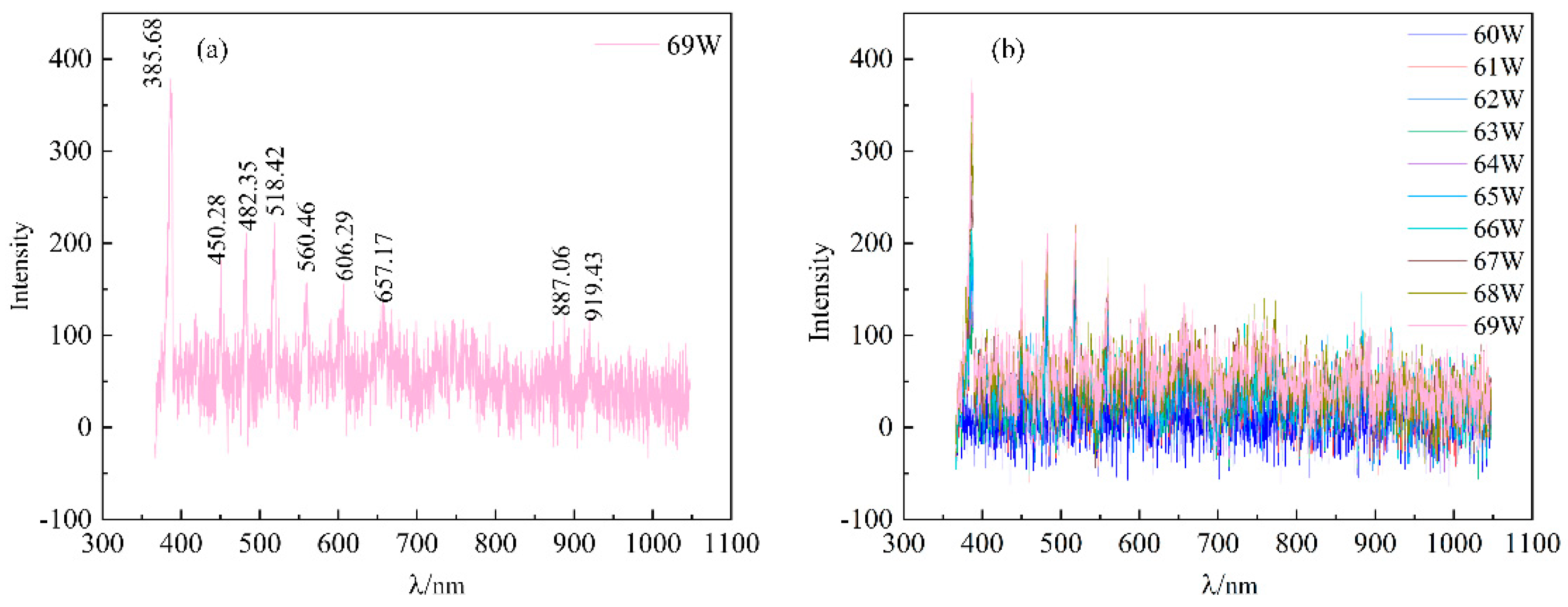Figure 2a represents the corresponding spectrum (with 2048 wavelengths) of 69 W after deducting background noise, showing that strong peaks appear at some specific wavelengths of 385.68, 450.28, etc. The spectral curves after deducting background noise collected under different rf powers from 60 to 69 W are shown in Figure 2b. It can be seen that the discharge intensity varies with rf power, i.e., the higher the rf power, the stronger the discharge intensity. In addition, it is seen that for a certain specific spectral curve, it is difficult to quickly identify the corresponding discharge power without a suitable model. In this paper, 60 to 69 W of rf power is only taken as an example to show the discharge macroscopic parameter. When the discharge power changes continuously, it is only necessary to update the dataset, and retrain and test the model. The model still has the ability to learn and recognize spectral features under different parameters; therefore, the discrete values of rf discharge power will not limit the application of the model.

When considering the model building and dataset construction, the file sizes of different formats should be compared. Compared with the collected spectral data files (in csv format), glow images (in bmp or jpg format) and the plotted spectral curve graphs (in png format) tend to have larger file sizes and more complexity. If using glow images and the plotted spectral curve graphs to build a dataset, it is necessary to construct a complicated 2D convolutional neural network. Meanwhile, for the spectral data file in csv format, because of its obviously smaller file size and the 1D data, only a 1D convolutional neural network is required. For example, the data for 10 spectral curves in csv format are 18 kb, while the data of the same 10 spectral curves are plotted as a graph in png format with a file size of 172 kb for the resolution of 300 dpi and 297 kb for the resolution of 600 dpi. In addition, the spectral data offer flexibility in terms of storage formats, ranging from simple integers to complex float point numbers. Its flexibility allows the numerical data to be adapted to the needs of a variety of applications, and the precise numerical representation of the data helps to achieve greater accuracy in data analysis and processing tasks. Thus, the 1D spectral data in csv format were used to construct the dataset and be recognized by our proposed 1D model as presented in this paper. For the construction of the ethylene spectral dataset, the data file of 8343 spectral curves was collected under different rf power, as shown in

Table 1. Dataset of spectra under different rf discharge powers.

Class	Ethylene Pressure (Pa)	Number of Spectral Curves	rf Power (W)	Label
1	190	790	60	0
2		860	61	1
3		919	62	2
4		835	63	3
5		861	64	4
6		820	65	5
7		807	66	6
8		814	67	7
9		819	68	8
10		818	69	9

. The total data files for the collected spectral curves can be classified into 10 classes with different labels corresponding to different rf powers. In the constructed dataset, the data of 5840 (or 70%) spectral curves were used to train the proposed model and the data of the remaining 2503 (or 30%) spectral curves were used to test the model.

3. Network Structure

3.1. Overall Design Ideas

In this study, a 1D deep convolutional neural network was constructed for recognition of the ethylene spectral data. First, the spectral data files (in csv format) with different labels were input into the model for training to learn the data features. During the training process, the model was saved with updated parameters. When the accuracy and loss reached the expected values after multiple iteration training, the trained model was ultimately saved for later use. Then, each spectral datum in the test dataset was input into the saved model to output the recognized label value (i.e., the rf power). 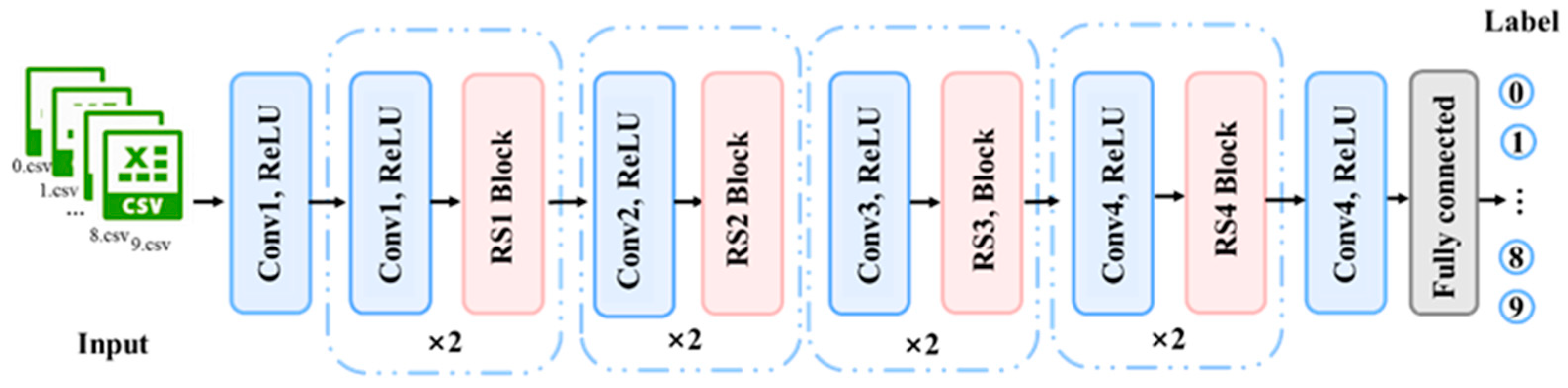Figure 3 shows the constructed model structure, which is mainly composed of the convolution layers and residual shrinkage (RS) blocks, marked by dashed lines. The RS block is composed of global average pooling, two fully connected layers, ReLU, and Sigmoid activation function. The model input size is 2048 × 1, and all the convolutional kernel sizes for Conv1-Conv4 in the blocks are 3 × 3 with the stride of 1 (there are two convolution layers with the same name of Conv1, meaning the same parameter in these two layers). The number of filters for Conv1-Conv4 and RS1-RS4 are 32, 64, 128, and 256, respectively. The last layer is the fully connected layer with the activation function of Sigmoid for the category of the output label.

This network not only contributes to the application of deep convolutional neural networks in 1D complex plasma data recognition tasks, but also innovates and improves the structure and learning mechanism of deep neural networks at the theoretical level by introducing residual blocks to solve the problem of gradient disappearance in deep networks to successfully train deeper structures and by introducing soft thresholding to dynamically adjust the weight of features according to the importance of features, thus suppressing unimportant features and strengthening key features. These theoretical contributions not only help to improve the performance of deep convolutional neural network models, but also provide new ideas and directions for the development of deep networks. Since the plasma spectral data is 1D, this model uses a 1D convolution kernel to process such data, which enables the network to capture local 1D features more efficiently. This model expands the application range of deep convolutional neural networks in signal processing, fault diagnosis, time series analysis, and other fields.

Since the plasma spectral data are 1D, this model uses 1D convolution to process such data, which enables the network to capture local 1D data features more efficiently. It should be pointed out that the input file in this paper is in csv format, not in an image format, which can be shown from the input files (0.csv–9.csv) in Figure 3. Due to the fact that the input spectral data file in csv format is 1D and significantly smaller than that in 2D images, the recognition efficiency of the model can be greatly improved.

The structural parameters that need to be adjusted include the kernel size, channel and step size of the convolution, etc. The selection and adjustment of these parameters have an important impact on the performance of the model. The structural parameters of the model are determined by continuous trial and adjustment according to the input data characteristics to improve the performance of the convolutional neural network. The detailed parameters in the proposed network for the input, operation, and output of the model are shown in

Table 2. The parameters in the network structure (RS: residual shrinkage; Conv: convolution; GAP: global average pooling; FC: full connection; S: stride; BN: batch normalization; CT: calculate thresholds; ST: soft thresholding; Add: add to the feature map of the residual branch).

Layer		Input Size	Kernel Size	Channel	Padding	Operation	Output Size
Input		2048 × 1	--	1	-	--	--
Conv1		2048 × 32	3 (S = 1)	32	same	Conv; BN; ReLU	2048 × 32
	Conv1	2048 × 32	3 (S = 1)	32	same	Conv; BN; ReLU	2048 × 32
	Conv1	2048 × 32	3 (S = 1)	32	same	Conv; BN; ReLU	2048 × 32
	GAP	2048 × 32	--	32	--	--	1 × 32
	FC	1 × 32	1 × 1	32	--	ReLU	1 × 32
RS1	FC	1 × 32	1 × 1	32	--	Sigmoid	1 × 32
	CT	1 × 32	--	32	--	--	1 × 32
	ST	1 × 32	1 × 1	32	--	--	2048 × 32
	Add	2048 × 32	--	32	--	--	2048 × 32
Conv2		2048 × 32	3 (S = 1)	64	same	Conv; BN; ReLU	2048 × 64
	Conv2	2048 × 64	3 (S = 1)	64	same	Conv; BN; ReLU	2048 × 64
	Conv2	2048 × 64	3 (S = 1)	64	same	Conv; BN; ReLU	2048 × 64
	GAP	2048 × 64	--	64	--	--	1 × 64
	FC	1 × 64	1 × 1	64	--	ReLU	1 × 64
RS2	FC	1 × 64	1 × 1	64	--	Sigmoid	1 × 64
	CT	1 × 64	--	64	--	--	1 × 64
	ST	1 × 64	1 × 1	64	--	--	2048 × 64
	Add	2048 × 64	--	64	--	--	2048 × 64
Conv3		2048 × 64	3 (S = 1)	128	same	Conv; BN; ReLU	2048 × 128
	Conv2	2048 × 128	3 (S = 1)	128	same	Conv; BN; ReLU	2048 × 128
	Conv2	2048 × 128	3 (S = 1)	128	same	Conv; BN; ReLU	2048 × 128
	GAP	2048 × 128	--	128	--	--	1 × 128
	FC	1 × 128	1 × 1	128	--	ReLU	1 × 128
RS3	FC	1 × 128	1 × 1	128	--	Sigmoid	1 × 128
	CT	1 × 128	--	128	--	--	1 × 128
	ST	1 × 128	1 × 1	128	--	--	2048 × 128
	Add	2048 × 128	--	128	--	--	2048 × 128
Conv4		2048 × 128	3 (S = 1)	256	same	Conv; BN; ReLU	2048 × 256
	Conv4	2048 × 256	3 (S = 1)	256	same	Conv; BN; ReLU	2048 × 256
	Conv4	2048 × 256	3 (S = 1)	256	same	Conv; BN; ReLU	2048 × 128
	GAP	2048 × 256	--	256	--	--	1 × 256
	FC	1 × 256	1 × 1	256	--	ReLU	1 × 256
RS4	FC	1 × 256	1 × 1	256	--	Sigmoid	1 × 256
	CT	1 × 256	--	256	--	--	1 × 256
	ST	1 × 256	1 × 1	256	--	--	2048 × 256
	Add	2048 × 256	--	256	--	--	2048 × 256
Conv4		2048 × 256	3 (S = 1)	256	same	Conv; BN; ReLU	2048 × 256
FC		2048 × 256	1 × 1	10	--	Softmax	1 × 10

.

3.2. Soft Thresholding

In the acquisition of plasma spectral data, there is often a lot of noise, which will interfere with the feature extraction and pattern recognition of the signal. When traditional networks process the signal with strong noise, it will be disturbed by the noise, which leads to the deterioration of the recognition performance. The model processes the input data by introducing a soft threshold function, which enables the network to adaptively learn and adjust the threshold of each sample. This soft thresholding mechanism can filter out noise-related features effectively and retain useful information related to tasks, so as to improve the recognition ability of noisy data. Compared with the traditional fixed threshold method, the soft threshold function in this network can adaptively set the threshold according to the characteristics of each sample. The ability of adaptive threshold setting enables the model to better adapt to data with different noise levels and distributions, and improves the generalization performance of the model.

Soft thresholding segmentation is a crucial step in many signal denoising methods. However, in classical wavelet thresholding, the design of filters requires a significant amount of expertise in signal processing, which is a challenging problem. Deep learning provides a novel approach to address this problem by using gradient descent algorithms to automatically learn filters instead of them being manually designed by experts. Therefore, the combination of soft thresholding and deep learning is an effective method for removing noise-related information and constructing highly discriminative features. The formula for soft thresholding can be represented as Equation (1).

$$y=\left\{\begin{array}{c}x-\tau x>\tau \\ 0-\tau \le x\le \tau \\ x+\tau x<-\tau \end{array}\right.,$$

(1)

where $x$, $y$, and $\tau$ represent the input feature, output feature and threshold (constant value during the training and test), respectively, and all of these three parameters are positive values. Soft thresholding is used to convert the near-zero features to zeros. From Equation (1), it can be observed that the derivative of the output $y$ with respect to the input $x$ is either 1 or 0, which can be represented as Equation (2) and mitigate the issues of gradient vanishing and exploding.

$$\frac{\partial y}{\partial x}=\left\{\begin{array}{c}1x>\tau \\ 0-\tau \le x\le \tau \\ 1x<-\tau \end{array}\right.$$

(2)

3.3. The Residual Shrinkage Block

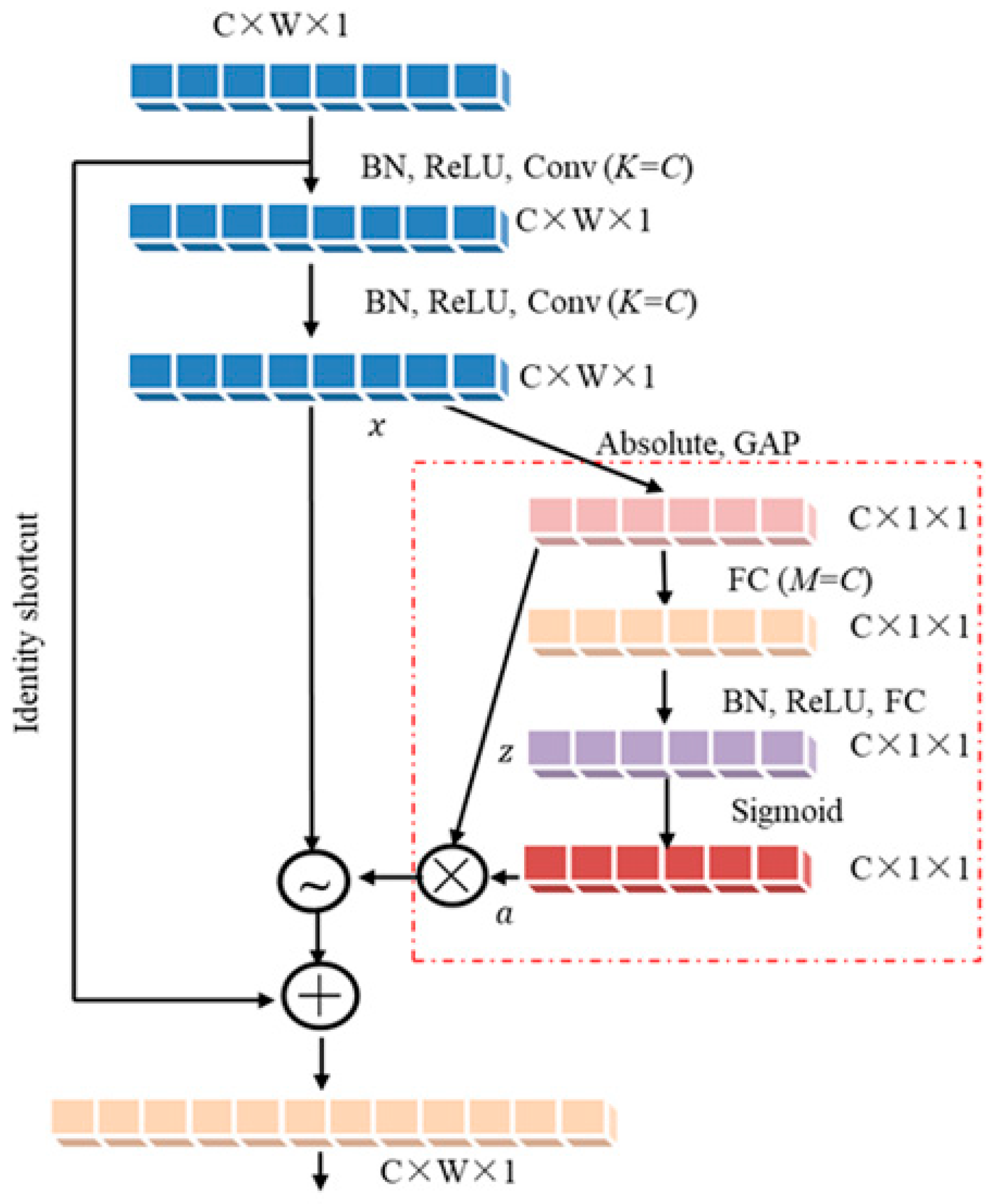
Figure 4 is a residual shrinkage block with channel thresholds, in which $K$ is the number of convolutional kernels in the convolutional layer, $M$ is the number of neurons in the FC layer, and $C$, $W$, and 1 in $C\times W\times 1$ are the indicators of the number of channels, width, and height of the feature map, respectively. $x$, $z$, and $\alpha$ are the indicators of the feature maps to be used when determining thresholds. The first two convolution layers, two batch normalization, and two activation functions transform the characteristics of redundant information into values close to zero, but transform useful features into values far from zero, which is then propagated into the two layers of the FC layer with multiple neurons (the number of neurons equals the number of channels in the input feature map). The output value of the $c$th channel of the FC layer is scaled to a range of (0, 1) by Equation (3), which automatically learns a set of thresholds. Redundant features are eliminated and useful features are retained using soft thresholding.

$${\alpha }_c=\frac{1}{1+e^{-z_c}}$$

(3)

where $-z_c$ and ${\alpha }_c$ are the features of the $c$th neuron and the $c$th scaling parameter, respectively. The threshold value, ${\tau }_c$, is calculated in Equation (4).

$${\tau }_c={\alpha }_c·\genfrac{}{}{0pt}{}{average}{i,j}\left|x_{i,j,c}\right|,$$

(4)

${\tau }_c$ is the threshold of the $c$th channel of the feature map. $i$, $j,$ and $c$ represent the dimensions of width, height, and channel of the feature $x$, respectively. $\genfrac{}{}{0pt}{}{average}{i,j}\left|x_{i,j,c}\right|$ means the average of the feature responses for each channel, which is used for the subsequent threshold calculation and channel weight adjustment.

3.4. Algorithmic Innovations

Firstly, the network solves the problem of gradient disappearance in deep neural networks by introducing residual connections, which allows the network to learn the residuals between inputs and outputs, helps the network to better propagate gradients during training, and enables deeper network structures to be trained. This structure is essential for capturing complex and abstract features.

Then, there was the introduction of a soft thresholding mechanism, a non-linear transformation for adaptive scaling of a feature map during feature learning. Through soft thresholding, the network can dynamically adjust the weight of features, suppress unimportant features, and enhance key features. This mechanism is particularly effective for dealing with the signals with noise or complex data because it can reduce noise interference of feature representations and improve the performance of the model.

Finally, the adaptive feature learning process is realized by combining residual learning and soft thresholding. This adaptability allows the network to dynamically adjust the feature representation according to different tasks and data characteristics, so as to extract and retain the features that are important to the recognition task more effectively. In addition, the design of the network also takes into account the characteristics of tasks and data, and uses a 1D convolution kernel and adaptive feature learning to optimize the performance of the model, so as to improve the classification accuracy.

On the whole, this network structure combines two mechanisms of residual learning and soft thresholding, which are designed to improve the feature learning ability of deep neural networks on complex and noisy data and improve the recognition accuracy.

4. Results and Analysis

4.1. Evaluation Indicators

In this experiment, accuracy, precision, recall, F1-Score, and confusion matrix were used as evaluation indicators and cross-entropy was used as the loss function. They are defined as follows.

$$Accuracy=\frac{TP+TN}{TP+FP+TN+FN},$$

(5)

$$Averageprecision=1/N{\sum }_{i=1}^N\frac{{TP}_i}{{(TP}_i+{FP}_i)}$$

(6)

$$Averagerecall=1/N\sum _{i=1}^N\frac{{TP}_i}{{(TP}_i+{FN}_i)},$$

(7)

$$F1\text{-}Score=1/N\sum _{i=1}^N\frac{2{{TP}_i}^2}{{TP}_i(2{TP}_i+{FP}_i+{FN}_i)},$$

(8)

$$Loss=-\frac{1}{N}\sum _x\left[y\mathrm{l}\mathrm{n}{y}^{\prime }+\left(1-y\right)\ln \left(1-y^{\prime }\right)\right],$$

(9)

where $N$ is the number of the samples, $y$ and $y^{\prime }$ denote the expected and actual output. True positive ($TP$) indicates that a case is predicted to be positive and is actually positive. False positive ($FP$) expresses being predicted as positive, but is a negative example. True negative ($TN$) means being predicted to be negative and is actually a negative case. False negative ($FN$) is where a predicted negative case is actually a positive example.

4.2. Experimental Environment and Hyper Parameter Selection

The hardware configuration of the computer used in the experiment was a 64-bit Windows 11 system, Intel(R) Core (TM) i5-11400F (2.59 GHz), GeForce RTX 3060. For software, Anaconda 4.10.3 was used as the development platform. Pytorch 1.9.0 was used as the deep learning open-source framework.

The selection and adjustment of the hyperparameters have an important impact on the performance of the model. The parameters that need to be adjusted include the learning rates, batch sizes, epochs, optimizer, etc. The hyperparameters of the model were determined by continuous trial and adjustment according to the output data characteristics to improve the performance of the convolutional neural network. As can be seen from

Table 3. Effects of different learning rates on the evaluation indicators.

Learning Rate	Accuracy	Precision	Recall	F1-Score
1.0 × 10−3	0.8076	0.8081	0.8076	0.8078
1.0 × 10−4	0.9466	0.9472	0.9466	0.9468
1.0 × 10−5	0.9844	0.9838	0.9834	0.9836
1.0 × 10−6	0.9309	0.9308	0.9303	0.9305

,

Table 4. Effects of different batch sizes on the evaluation indicators.

Batch Size	Accuracy	Precision	Recall	F1-Score
8	0.9844	0.9838	0.9834	0.9836
16	0.9421	0.942	0.9408	0.9414
32	0.9228	0.9227	0.9222	0.9224
64	0.9166	0.9165	0.9159	0.9162

,

Table 5. Effect of different epochs on the evaluation indicators.

Epoch	Accuracy	Precision	Recall	F1-Score
30	0.9377	0.9385	0.9377	0.9381
40	0.9475	0.9477	0.9475	0.9476
50	0.9844	0.9838	0.9834	0.9836
60	0.9553	0.9559	0.9553	0.9556

and

Table 6. Effect of different optimizers on the evaluation indicators.

Optimizer	Accuracy	Precision	Recall	F1-Score
Adam	0.9844	0.9838	0.9834	0.9836
SGD	0.8892	0.8943	0.8854	0.8898
Adagrad	0.944	0.9677	0.8941	0.9294
Nadam	0.9745	0.9681	0.9742	0.9711

, when the learning rate, batch size, epochs, and optimizer are 1.0 × 10⁻⁵, 8, 50, and Adam, respectively, the recognition effect of this model is the best with the highest accuracy, precision, recall, and F1-Score, respectively, which are marked in bold.

4.3. Experimental Results

Figure 5 shows the curve of accuracy and loss changing as epochs during the model training and testing. It can be seen that both the accuracy curves of training and testing rise rapidly when the epoch is within 1–9. When the epoch is in the range of 9–41, both the accuracy curves of training and testing show the fluctuation, especially for the testing curve with a fluctuation between 91.5% and 98.3%. When the epoch is greater than 41, both the training accuracy and test accuracy gradually stabilize at above 98%. Figure 5b shows the loss curves of training and testing changing as epochs. One can see that both the loss curves of training and testing decline rapidly to below 0.2 when the epoch is in the range of 1–9. When the epoch is in the range of 9–44, both the loss curves of training and testing show the fluctuations. When the epoch is greater than 44, both the loss value of training and testing is only about 5%, indicating that the model has reached stability. During training of the model, the convergence speed of networks refers to the time required for the network to reach the optimal solution during training. In this experiment, the convergence rate of our model is 157 min, corresponding to 44 epochs.

A confusion matrix, also known as error matrix, is a tool used to evaluate the performance of classification models, which can visually display the classification results of a model for different categories. It summarizes the data in matrix form based on two criteria: the actual class (i.e., the true label) and the class predicted by the recognition model (the predicted label). Figure 6 shows the confusion matrix of our model for the test set of 10 classes of ethylene plasma spectra, in which the horizontal axis represents the predicted labels, and the vertical axis represents the true labels. Color depth represents the prediction accuracy value, and the darker the color, the higher the accuracy. In the ten classes, the recognition accuracy for all classes is higher than 95%, as indicated by the deep red color on the diagonal, indicating the effectiveness of the proposed model for recognizing ethylene plasma spectra.

The constructed dataset was also tested using different models, and the comparison of the evaluation indicators is shown in Figure 7, which indicates that all the four evaluation indicators by our model are the highest, i.e., our model has the best recognition effect on the ethylene discharge spectra.

For a more detailed comparison,

Table 7. Comparison of the evaluation indicators using different models and TOPSIS analysis.

Models	Accuracy	Precision	Recall	F1-Score	f-Value
AlexNet	0.6908	0.6924	0.6896	0.6923	0.0
1DCNN	0.7688	0.7699	0.7659	0.7678	0.263
Vgg13	0.7988	0.8012	0.7965	0.7988	0.368
ResNet18	0.8705	0.8715	0.8705	0.871	0.614
Ours	0.9844	0.9838	0.9834	0.9836	1.000

shows the values of the four evaluation indicators and the statistical TOPSIS analysis results using different models. It can be seen that the recognition accuracies for AlexNet, 1DCNN, Vgg13, and ResNet18 are 69.08%, 76.88%, 79.88%, and 87.05%, respectively. In comparison, our model achieves the accuracy of 98.44%, which is a significant improvement of 29.36%, 21.56%, 18.56%, and 11.39%, respectively, compared to AlexNet, 1DCNN, Vgg13, and ResNet18. TOPSIS is an effective multi-indicator evaluation method, by which the optimal and worst values for each indicator can be obtained from all the values of each indicator, and then the distances from the point corresponding to each evaluation value to the optimal and worst points are calculated to obtain the overall evaluation value (represented by f in this paper). The larger the f-value, the better the evaluation indicators. For Table 7, it can be seen that our model has the maximum f-value of 1.0, and AlexNet has the smallest f-value of 0, indicating that our model has the best comprehensive performance for these four evaluation indicators.

Table 8. Comparison of the parameter quantity and training duration on the constructed ethylene spectral dataset using different models (The same dataset was used in these models).

Models	Parameter Quantity (kB)	Training Duration (min)
AlexNet	61.44	5
1DCNN	85.71	5.9
Vgg13	121.36	4.5
ResNet18	184.7	29.5
Ours	2088.96	210

shows the comparison of the parameter quantity and training duration on the constructed ethylene spectral dataset using different models. It shows that our model has a larger parameter quantity (2088.96 kB) and longer training duration (210 min for training 50 epochs) than the other comparable models, which need to be further optimized in the future.

In order to verify the effectiveness of the method on public datasets, such as humidity datasets, wheat seed data (Kama, Rosa, and Canadian), and a Wisconsin breast cancer dataset,

Table 9. The recognition results of our model on three public datasets.

Dataset	Accuracy	Precision	Recall	F1-Score
Humidity (9 classes, 100 item/class)	1	1	1	1
Wheat Seeds (3 classes, 70 item/class)	0.9686	0.9671	0.9667	0.9668
Wisconsin Breast Cancer (2 classes, 357 item and 212 item)	0.97	0.97	0.97	0.97

presents the results of our model on these public datasets. It can be seen that the model achieves perfect recognition effect with all the evaluation indicators being 1.0 on the humidity dataset, and over 96% on both the wheat seed and Wisconsin breast cancer datasets. All the four evaluation indicators being 1.0 on the humidity dataset is mainly due to the significant difference between the data features of the nine classes, which is easy to be recognized.

5. Conclusions

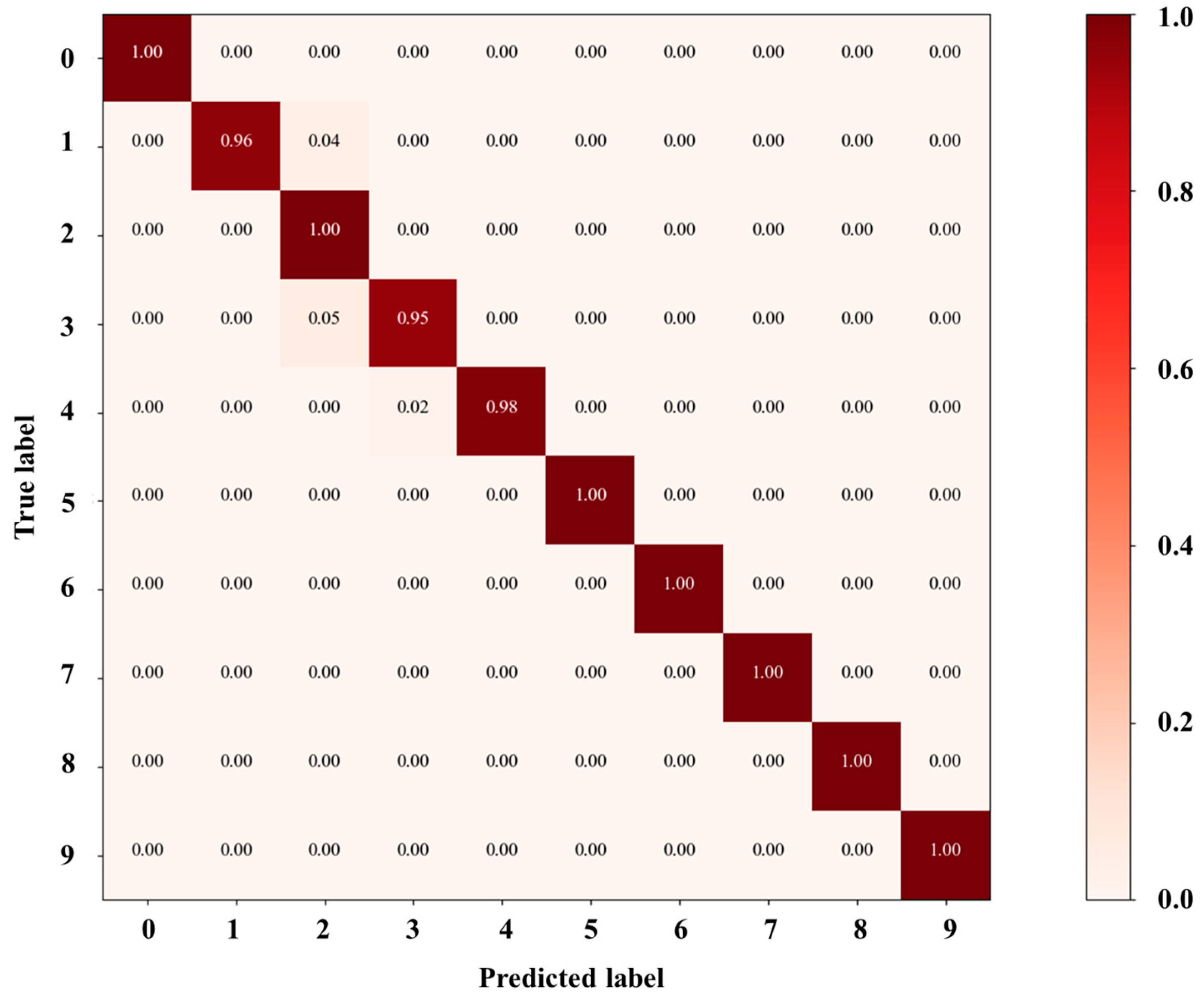
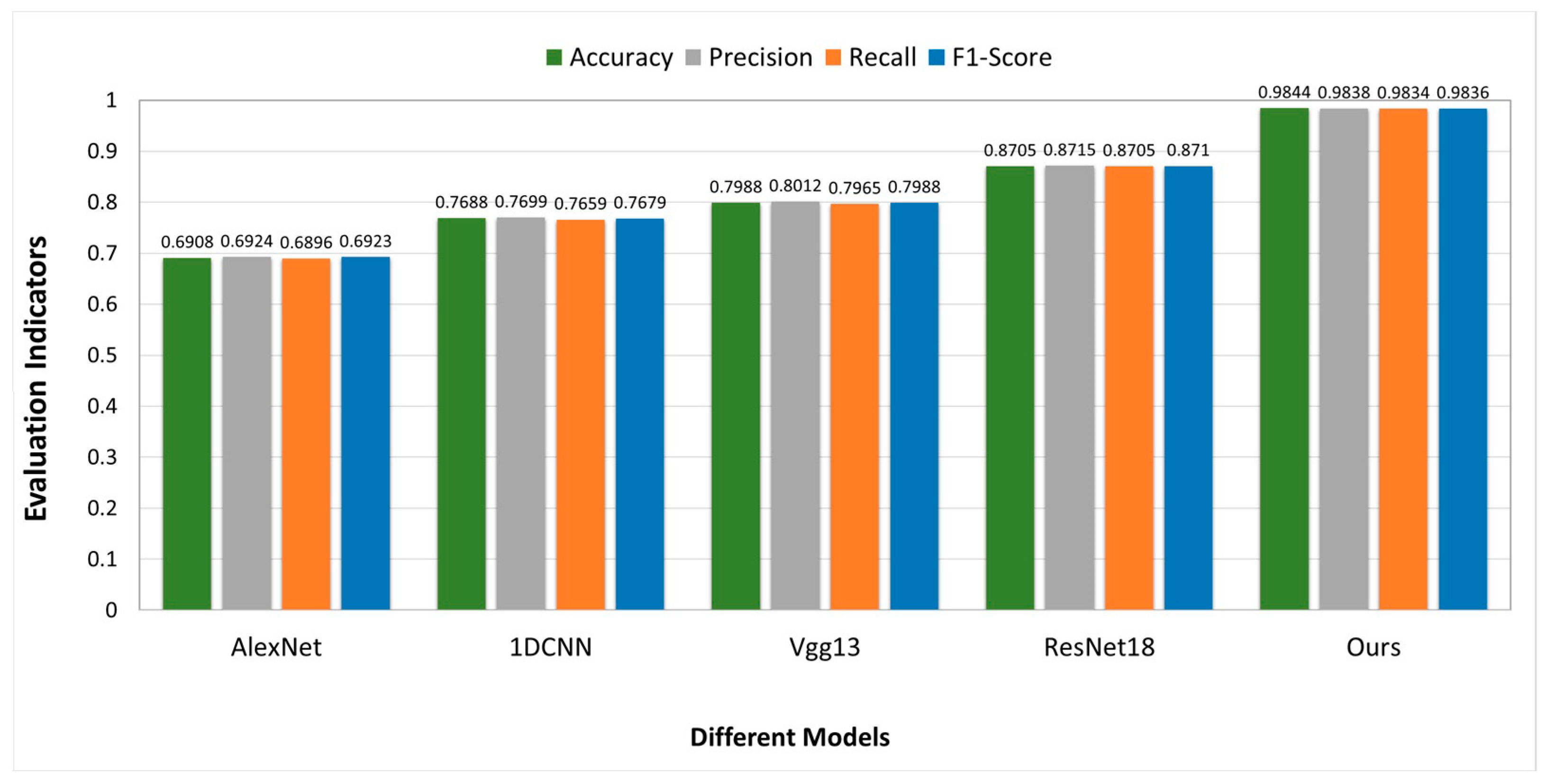
In this paper, the deep convolutional neural network was proposed for recognizing the macro parameters of discharge from the corresponding ethylene plasma spectrum. The proposed network has strong feature learning and extraction ability with a residual shrinkage block which finds the less important features through the attention mechanism and removes the unimportant information by embedding soft thresholds. In addition, a shortcut connection is added, allowing gradients to propagate directly from the input layer to the output layer, thereby effectively preserving important data features and improving the recognition accuracy. This model can effectively recognize ethylene plasma spectral data with all the four evaluation indicators of higher than 98%. Compared with four other classical recognition models, our model shows the best recognition performance. This model can not only recognize the macro plasma discharge parameters including rf power, gas pressure, gas ratio, and so on, but also plasma microscopic parameters including the temperatures and densities of electrons and ions corresponding to the spectra, which provides technical support for plasma spectrum diagnosis and plasma application in industry.

References

1. Huang, Y.M.; Yuan, Y.X.; Yang, L.J.; Wu, D.; Chen, S.B. Real-time monitoring and control of porosity defects during arc welding of aluminum alloys. J. Mater. Process. Technol. 2020, 286, 116832. [Google Scholar] [CrossRef]
2. Chiang, W.H.; Mariotti, D.; Sankaran, R.M.; Eden, J.G.; Ostrikov, K. Microplasmas for advanced materials and devices. Adv. Mater. 2020, 32, 1905508. [Google Scholar] [CrossRef] [PubMed]
3. Sikdar, S.; Menezes, P.V.; Maccione, R.; Jacob, T.; Menezes, P.L. Plasma electrolytic oxidation (PEO) process—Processing, properties, and applications. Nanomaterials 2021, 11, 1375. [Google Scholar] [CrossRef] [PubMed]
4. Karadag, B.; Cho, S.; Funaki, I. Thrust performance, propellant ionization, and thruster erosion of an external discharge plasma thruster. J. Appl. Phys. 2018, 123, 153302. [Google Scholar] [CrossRef]
5. Zhu, X.M.; Wang, Y.F.; Wang, Y.; Yu, D.R.; Zatsarinny, O.; Bartschat, K.; Tsankov, T.V.; Czarnetzki, U. A xenon collisional-radiative model applicable to electric propulsion devices: II. Kinetics of the 6s, 6p, and 5d states of atoms and ions in Hall thrusters. Plasma Sources Sci. Technol. 2019, 28, 105005. [Google Scholar] [CrossRef]
6. Green, D.S.; Hatate, H.; Oga, R.; Yamamoto, S.; Fujiwara, Y.; Takeda, Y.; Noda, H.; Urisu, T. Materials and integration strategies for modern RF integrated circuits. In Proceedings of the 2014 IEEE Compound Semiconductor Integrated Circuit Symposium (CSICS), La Jolla, CA, USA, 19–22 October 2014; pp. 1–4. [Google Scholar] [CrossRef]
7. Huff, M. Recent advances in reactive ion etching and applications of high-aspect-ratio microfabrication. Micromachines 2021, 12, 991. [Google Scholar] [CrossRef]
8. Min, B.G.; Lee, J.M.; Yoon, H.S.; Chang, W.J.; Park, J.Y.; Kang, D.M.; Chang, S.J.; Jung, H.W. Analysis of issues in gate recess etching in the InAlAs/InGaAs HEMT manufacturing process. ETRI J. 2023, 45, 171–179. [Google Scholar] [CrossRef]
9. Donnelly, V.M.; Kornblit, A. Plasma etching: Yesterday, today, and tomorrow. J. Vac. Sci. Technol. A 2013, 31, 050825. [Google Scholar] [CrossRef]
10. Grigoriev, S.; Dosko, S.; Vereschaka, A.; Zelenkov, V.; Sotova, C. Diagnostic techniques for electrical discharge plasma used in PVD coating processes. Coatings 2023, 13, 147. [Google Scholar] [CrossRef]
11. Edy, R.; Huang, G.S.; Zhao, Y.T.; Guo, Y.; Zhang, J.; Mei, Y.F.; Shi, J.J. Influence of reactive surface groups on the deposition of oxides thin film by atomic layer deposition. Surf. Coat. Technol. 2017, 329, 149–154. [Google Scholar] [CrossRef]
12. Yang, J.; McArdle, C.; Daniels, S. Dimension reduction of multivariable optical emission spectrometer datasets for industrial plasma processes. Sensors 2014, 14, 52–67. [Google Scholar] [CrossRef]
13. Engeln, R.; Klarenaar, B.; Guaitella, O. Foundations of optical diagnostics in low temperature plasmas. Plasma Sources Sci. Technol. 2020, 29, 063001. [Google Scholar] [CrossRef]
14. Tang, X.L.; Qiu, G.; Yan, Y.H.; Shi, Y.C.; Feng, P.X. Spectral diagnosis of dielectric barrier plasma discharge at atmospheric pressure and its application to surface modification of materials. Spectrosc. Spect. Anal. 2004, 24, 1437–1440. [Google Scholar] [CrossRef]
15. Chen, B.; Yao, Y.Z.; Tan, C.W.; Huang, Y.H.; Song, X.G.; Feng, J.C. Investigation of the correlation between plasma electron temperature and quality of laser additive manufacturing process. In Transactions on Intelligent Welding Manufacturing; Springer: Berlin/Heidelberg, Germany, 2017; pp. 60–74. [Google Scholar] [CrossRef]
16. Jeong, B.Y.; Kim, M.H. Effects of the process parameters on the layer formation behavior of plasma nitrided steels. Surf. Coat. Technol. 2001, 141, 182–186. [Google Scholar] [CrossRef]
17. Zille, A.; Oliveira, F.R.; Souto, A.P. Plasma treatment in textile industry. Plasma Process. Polym. 2014, 12, 98–131. [Google Scholar] [CrossRef]
18. Vergunova, G.A.; Ivanov, E.M.; Rozanov, V.B. Emission spectra of a plasma observed upon irradiation of solid targets by high-intensity ultrashort laser pulses. Quantum Electron. 2003, 33, 105. [Google Scholar] [CrossRef]
19. Bai, L.; Zhang, D.M.; Lv, Q.; Zhang, L.L.; Wang, Y.K.; Xu, Y.Y. An improved collision-radiation model of the OH spectrum in the ultraviolet band. J. Quant. Spectrosc. Radiat. Transf. 2021, 271, 107671. [Google Scholar] [CrossRef]
20. Stafford, L.; Khare, R.; Donnelly, V.M.; Margot, J.; Moisan, M. Electron energy distribution functions in low-pressure oxygen plasma columns sustained by propagating surface waves. Appl. Phys. Lett. 2009, 94, 021503. [Google Scholar] [CrossRef]
21. Wang, Q.; Koleva, I.; Donnelly, V.M.; Economou, D.J. Spatially resolved diagnostics of an atmospheric pressure direct current helium microplasma. J. Phys. D Appl. Phys. 2005, 38, 1690. [Google Scholar] [CrossRef]
22. Hansen, S.B.; Bauche, J.; Bauche-Arnoult, C.; Gu, M.F. Hybrid atomic models for spectroscopic plasma diagnostics. High Energy Density Phys. 2007, 3, 109–114. [Google Scholar] [CrossRef]
23. Wang, C.Y.; Ko, T.S.; Hsu, C.C. Interpreting convolutional neural network for real-time volatile organic compounds detection and classification using optical emission spectroscopy of plasma. Anal. Chim. Acta. 2021, 1179, 338822. [Google Scholar] [CrossRef]
24. Wang, C.Y.; Hsu, C.C. Development and testing of an efficient data acquisition platform for machine learning of optical emission spectroscopy of plasmas in aqueous solution. Plasma Sources Sci. Technol. 2019, 28, 105013. [Google Scholar] [CrossRef]
25. Kruger, F.; Gergs, T.; Trieschmann, J. Machine learning plasma-surface interface for coupling sputtering and gas-phase transport simulations. Plasma Sources Sci. Technol. 2019, 28, 035002. [Google Scholar] [CrossRef]
26. Grelier, E.; Mitteau, R.; Moncada, V. Deep learning-based process for the automatic detection, tracking, and classification of thermal events on the in-vessel components of fusion reactors. Fusion Eng. Des. 2023, 192, 113636. [Google Scholar] [CrossRef]
27. Shin, H.; Oh, S.; Hong, S.; Kang, M.; Kang, D.; Ji, Y.; Choi, B.H.; Kang, K.W.; Jeong, H.; Park, Y.; et al. Early-stage lung cancer diagnosis by deep learning-based spectroscopic analysis of circulating Exosomes. ACS Nano 2020, 14, 5435–5444. [Google Scholar] [CrossRef] [PubMed]
Figure 1. Top view of the experimental setup and A, B, A’ and B’ are windows. (a) ethylene discharge image taken from window A (b).
Electronics 13 00983 g001
Figure 2. (a) Ethylene discharge spectra at different rf powers of 69 W and (b) 60−69 W.
Electronics 13 00983 g002
Figure 3. The model structure.
Electronics 13 00983 g003
Figure 4. Residual shrinkage block.
Electronics 13 00983 g004
Figure 5. Accuracy (a) and loss (b) curve change as epochs during training and testing.
Electronics 13 00983 g005
Figure 6. The confusion matrix of our model on the test set of the ethylene plasma spectra.
Electronics 13 00983 g006
Figure 7. Comparison of evaluation indicators using different experimental methods.
Electronics 13 00983 g007