Control Performance Requirements for Automated Driving Systems

Abstract

This research investigates the development of risk-based performance requirements for the control of an automated driving system (ADS). The proposed method begins by determining the target level of safety for the virtual driver of an ADS. The underlying assumptions are informed by existing data. Next, geometric models of the road and vehicle are used to derive deterministic performance levels of the virtual driver. To integrate the risk and performance requirements seamlessly, we propose new definitions for errors associated with the planner, pose, and control modules. These definitions facilitate the derivation of stochastic performance requirements for each module, thus ensuring an overall target level of safety. Notably, these definitions enable real-time controller performance monitoring, thus potentially enabling fault detection linked to the system’s overall safety target. At a high level, this approach argues that the requirements for the virtual driver’s modules should be designed simultaneously. To illustrate this approach, this technique is applied to a research project available in the literature that developed an automated steering system for an articulated bus. This example shows that the method generates achievable performance requirements that are verifiable through experimental testing and highlights the importance in validating the underlying assumptions for effective risk management.

1. Introduction

An automated driving system (ADS), as defined in [1] (i.e., Levels 3 to 5), have the potential to reduce on-road collisions and fatalities. Many manufacturers today provide a wide variety of active safety systems that fall under SAE Level 2, where a part of the dynamic driving task is automated by the system [2]. Only a handful of companies in the United States have demonstrated city-scale Level 3 or Level 4 deployment of ADS [3,4]. The work presented subsequently is most readily applicable from Level 3 to Level 5 systems, but Level 2 systems may also benefit from parts of this work.

Proving that the promised safety benefit is achieved remains a major challenge for the industry [3,4]. This is, in part, due to the wide range of functions the ADS must perform in highly uncertain and dynamic environments. To automate the entire dynamic driving task, difficult challenges in perception, planning, and control must be solved.

Conventional techniques for solving complex, interconnected challenges come from taking a systems engineering approach. Such techniques have been widely adopted in the aerospace industry [5]. The automotive industry has also adopted systems engineering approaches to achieve highly reliable and safe vehicles [6]. A common characteristic of these approaches is to distill products into subsystems and interfaces. One of the early proposals for a full ADS system separated several functions into modules, or subsystems [7]. More modern ADS architectures now largely follow the Sense-Plan-Act paradigm that is common in the field of robotics.

This approach provides a framework so that the various ADS challenges can be more precisely defined and subsequently solved. The current state-of-the-art standards are the ISO 26262 and ISO/DIS 21448 standards [8,9]. However, they are not comprehensive enough to facilitate the entire development, testing, and proof of safe ADS. The authors of [10] suggest that these standards are too subjective. The authors of [10] provide a more objective method to compute the system’s risk. The authors in [11] criticize claims of proving safety based on empirical testing on public roads, because the difficulty of those empirical tests is often low and lacks variety. In other words, it is not just the distance traveled but also the difficulty of that distance that matters when proving an ADS is safe. A useful overview of how the ISO 26262 can be applied to an ADS and extended to improve the safety of an ADS can be found in [12].

While these standards and their extensions provide methods for designing tests and quantifying risks, they do not equip a control engineer with a set of quantifiable performance metrics for a control system. Instead, they provide more general frameworks that can be used to derive requirements on reliability and to quantify risk. The control engineer is then tasked with interpreting these standards in such a way as to develop performance requirements. By performance requirements, we refer to the set of quantified metrics that can aid in deciding if a controller will provide sufficiently safe functionality or if a controller is sufficiently tuned. Common performance requirements in linear control systems are rise time, percent overshoot, steady state error, etc. These are examples of metrics that are specific to linear control systems, and while they can be applied to more complicated systems, we are primarily focused on proposing metrics that are more general.

Such requirements can be put in the context of the standard “V” model frequently used in systems engineering and in the ISO 26262. The ISO 26262 provides guidelines for designing tests and verifying the correct implementation of the designed controller. However, these guides are more focused on the software implementation and the hardware on which that software runs. They are not focused on the performance of the correctly implemented controller. To put it another way, even after satisfying the ISO 26262 guidelines on software implementation, the control engineer needs to also prove that control performance will ensure safe operation in the ADS’s operational design domain.

Typically, such evaluations are based on metrics of the controller’s performance. In practice, the derivation of such characteristics is often ad hoc and iterative. There is therefore an open question of how to use an ADS’s desired risk to derive quantifiable control system performance requirements. This work is focused primarily on answering this question. In the process of doing so, several other observations are made, which are summarized in the list of contributions at the end of this section.

Before introducing this methodology, it is worth discussing desired characteristics of such a method:

• The control system requirements should apply to all types of controllers (i.e., fuzzy logic, robust, model predictive control, nonlinear, etc.).
• Requirements should be independent of the vehicle, operational design domain, and dynamic driving task. Therefore, a methodology that has this characteristic can be used to determine which operational design domains the ADS can safely operate in and which it cannot.
• Requirements should account for uncertainty (i.e., specify the maximum allowable error or a desired distribution of errors). The methodology proposed in this paper accounts for the uncertainty in the operational design domain and dynamic driving task by providing requirements in the form of characteristics of a stochastic distribution. This also aids in their ability to be verified with experimental data, which is demonstrated in Section 3.1.
• The control requirements should be specific enough to provide binary determinations of the controller’s safety. For instance, it should provide a maximum standard deviation of the lateral error so that if the tested controller’s distribution does not meet this requirement, it is easy to argue that the controller provides insufficient performance.

Most requirements for a controller have been based on some combination of values such as maximum lateral error, maximum lateral jerk, or maximum lateral acceleration [13,14,15]. Many papers that propose new lateral path tracking controllers do not present a required level of performance. Instead, they display experimental or simulation results as a comparison with one or more state-of-the-art controllers [15,16,17,18]. An engineer searching the literature for a controller is left guessing which controller, if any, is capable of composing a safe ADS. Without a predefined requirement, the control engineer is forced to resort to a trial-and-error design procedure, which can be costly, time-consuming, and hazardous. It is also common to include some requirements on comfort. However, this work is primarily concerned with safety and, therefore, the proposed methodology ignores comfort.

To the authors’ knowledge, no methodology with the above-desired characteristics exists that directly connects risk to control requirements. However, a closely related work is [19], which is concerned with deriving localization requirements. The methodology described in subsequent sections can be viewed as an extension of the one developed in [19].

This paper makes the following contributions:

• A new set of definitions is proposed for each module’s performance metrics. These definitions balance specificity and generality so that quantifiable requirements can be derived from each module’s performance while also being applicable to a wide range of module implementations. A consequence of these definitions is that their performances are interdependent. Therefore, this contribution makes the argument that performance requirements should be allocated to the planner, pose, and control modules simultaneously rather than being treated independently, as is done in [19].
• A new method is presented that directly links the desired safety of the VDS to the performance metrics of the planner, pose, and control modules.
• This work addresses a deficient assumption in [19]’s definitions underlying their risk allocation, which has the effect of making the method less overly conservative and therefore more practical.

At a high level, this paper proposes an approach to applying the method developed in [19] to the VDS. The geometric assumptions and terminology in [19] are briefly reviewed in Section 2.1. To apply this method to the VDS, we define individual tasks for the planner, pose, and control modules. These definitions permit the development of practical performance metrics. These definitions, along with an example risk allocation, are presented in Section 2.2. The result of formalizing these tasks is a simple, mathematical relationship between each module’s performance in the form of parameters for the distributions of distance and orientation measurements. Section 2.2 also presents examples of how to use this method on conventional passenger vehicles. A more involved example is developed in Section 3.1 that shows how to apply this method to unconventional vehicles. This case study further demonstrates that the method produces feasible requirements while highlighting potential shortcomings that engineers should be aware of when using this method. Finally, Section 4 summarizes this work’s results and discusses its limitations.

2. Materials and Methods

2.1. Terminology

Following the systems engineering approach, a convenient architecture for an ADS is to define a VDS and a vehicle system. The VDS is composed of the tasks that a human performs when manually driving. The vehicle system is composed of the physical vehicle and its low-level controllers. Typically, the VDS provides commands to the vehicle system similar to what a human would do when operating a vehicle (i.e., steering wheel angle, throttle percentage, brake percentage). This partition is useful because it allows ADS developers to leverage the design and manufacturing expertise of existing original equipment manufacturers. This leaves the ADS developers with more resources to dedicate to the VDS.

Figure 1 shows how the VDS is further broken into modules. Most modules in Figure 1 are wellpknown, except for the Pose module, which consumes both the sensor outputs and the localization output to provide feedback to the control module. Some architectures use the localization module instead. However, the remainder of this paper will assume the existence of the pose module. For architectures that do not use one, the following methods applied to the pose module can be directly applied to the localization module.

The use of concepts such as protection levels and availability is typically applied to localization technologies [19,20]. Here, we briefly introduce some of these concepts.

The distance between the vehicle’s true position and the localization’s estimate is called the actual error. The reliability of this localization estimate is specified as the protection level. When the protection level exceeds a prespecified bound, called an alert limit, the system is said to be unavailable. When the actual error is outside the protection level, but within the alert limit, the system is said to be misleading. Finally, when the actual error is outside both the protection level and the alert limit, the system is called hazardous. The Stanford diagram then describes these relationships visually [20]. These concepts have been successfully applied to the Wide Area Augmentation System [20], which improves GPS reliability and availability.

In [19], the concepts of protection levels and alert limits are applied to automotive localization systems. Alert limits are defined based on representing the vehicle as a two-dimensional rectangle bounded inside a lane with a constant radius. This is visually shown in Figure 2. The work of [19] further derives maximum protection levels as the maximum value of the instantaneous estimates of the vehicle’s position and orientation.

While these concepts are traditionally applied to safety-critical localization systems, they can also be applied to safety-critical systems more generally. In this work, we apply the concepts of alert limits and protection levels to the VDS. As will be shown, this results in more comprehensive performance requirements for several modules in the VDS. The underlying argument for this is that the performance of each module cannot be considered in isolation, as they are interdependent. However, this assertion relies on the definitions of each module’s performance metrics (which will be introduced in Section 2.2).

The method begins by redefining the distance components of the actual error as the distance between the vehicle and the center of the lane. The orientation components of the actual error are the relative angles between the vehicle and the lane heading (we will relax these definitions later so that they apply more broadly to other driving tasks such as collision avoidance). The protection levels are then a bounding of the actual error in terms of the vehicle’s lateral and longitudinal directions, as well as the vehicle’s yaw orientation. This is visually shown in Figure 3. The alert limit is simply the worst-case combination of the maximum protection levels, which can be represented by a rectangle with length y and width x within a lane of constant radius, as shown in Figure 2.

These new definitions provide a framework for determining when the VDS is available, misleading, and/or hazardous. When the system is within both the protection levels and the alert limits, the VDS is considered available. When the system is hazardous, a part of the vehicle is outside of the lane. When the system is misleading, the vehicle remains in the lane (alert limit), but one or more of the actual errors exceeds the protection levels. An example of how this can occur is when the lateral component of the actual error exceeds the lateral protection level, but the combination of all the actual error components (lateral, longitudinal, and yaw) result in the vehicle being within the alert limit. These definitions can then be directly related to fault detection and management as framed by the ISO 26262 and DIS 21448.

To compute the requirements for the alert limits and protections levels, we begin by relating the vehicle and lane geometry to alert limits. The lateral and longitudinal alert limits are computed with the following equations from [19]:

$$x=\sqrt{{(r+\frac{w}{2})}^2-{\left(\frac{y}{2}\right)}^2}+\frac{w}{2}-r$$

(1)

$$A{L}_{lat}=\frac{(x-w_v)}{2}$$

(2)

$$A{L}_{lon}=\frac{(y-l_v)}{2}$$

(3)

where $w_v$ is the vehicle’s width in meters, $l_v$ is the vehicle’s length in meters, ${AL}_{lat}$ is the lateral alert limit, ${AL}_{lon}$ is the longitudinal alert limit, and the remaining variables are as defined in Figure 2.

To demonstrate the application of Equations (1)–(3), we use the geometry of several vehicles that represent the passenger vehicle classes presented in

Table 1. Vehicle parameters for examples of passenger vehicles.

Vehicle Class	Vehicle Name	Width [m]	Length [m]
A	2019 Fiat 500	1.63	3.55
B	2019 Ford Fiesta Hatchback	1.72	4.06
C	2024 Mercedes Benz A-Class	1.80	4.55
J	2019 Jeep Cherokee	1.9	4.6

.

The Alert Limits are computed using parameters for a Jeep Cherokee and for freeway, interchange, arterial, collector, and local roads. The specifications are shown in Figure 4 and come from [19], where the local roads are assumed to be 3.0 m wide and have a minimum radius of curvature of 10 m. The results show that freeways are the least restrictive, while the local roads are the most restrictive.

The alert limits define only lateral and longitudinal limits. To incorporate yaw angle limits, protection levels are introduced. Protection levels define the maximum lateral and longitudinal position error and yaw angle error. Their combination defines a rotated rectangle that must be within the alert limits. While [19] includes vertical errors, we focus only on planar errors, because the VDS is typically incapable of controlling vertical movement (outside of vertical accelerations for comfort purposes).

The next step is to derive the equations governing the trade-off between lateral, longitudinal, and yaw protection levels. Using a small angle assumption and considering only planar components, the following can be derived:

$$\begin{array}{cc}\hfill {\delta }_{lat}+({\delta }_{lon}+\frac{l_v}{2}){\delta }_{\psi }& \le A{L}_{lat}\hfill \\ \hfill {\delta }_{lon}+({\delta }_{lat}+\frac{w_v}{2}){\delta }_{\psi }& \le A{L}_{lon}\hfill \end{array}$$

(4)

where ${\delta }_{lat}$ is the lateral protection level, ${\delta }_{lon}$ is the longitudinal protection level, and ${\delta }_{\psi }$ is the yaw protection level.

Next, by rearranging these equations and assuming equality instead of inequality, we obtain:

$$\left[\begin{array}{c}{\delta }_{lat}\\ {\delta }_{lon}\end{array}\right]={\left[\begin{array}{cc}1& {\delta }_{\psi }\\ {\delta }_{\psi }& 1\end{array}\right]}^{-1}\left[\begin{array}{c}A{L}_{lat}-\frac{l_v}{2}{\delta }_{\psi }\\ A{L}_{lon}-\frac{w_v}{2}{\delta }_{\psi }\end{array}\right]$$

(5)

After substituting Equations (1)–(3) in, the protection levels can be shown to be functions of y and ${\delta }_{\psi }$. It is useful to generate plots of the trade-off between each protection level as is done in Figure 5 for the Jeep Cherokee when ${\delta }_{\psi }$ = 0.05 rad and for a range of y. To use these curves, the engineer need only select a point along these curves, and all three of the protection levels are determined. If needed, the alert limits can then be computed from this selection.

Table 2. Alert limits and lateral protection level for example vehicles on arterial roads.

Vehicle	${\mathit{\delta }}_{\mathit{l}\mathit{a}\mathit{t}}$ [m]	${\mathit{\delta }}_{\mathit{l}\mathit{o}\mathit{n}}$ [m]	${\mathit{\delta }}_{\mathit{\psi }}$ [rad]	${\mathit{AL}}_{\mathit{lat}}$ [m]	${\mathit{AL}}_{\mathit{lon}}$ [m]
2019 Fiat 500	0.68	0.8	0.05	0.81	0.87
2019 Ford Fiesta Hatchback	0.62	0.8	0.05	0.76	0.87
2024 Mercedes Benz A-Class	0.56	0.8	0.05	0.71	0.87
2019 Jeep Cherokee	0.50	0.8	0.05	0.66	0.87

shows the computed alert limits when ${\delta }_{\psi }$ is 0.05 rad and ${\delta }_{lon}$ is 0.8 m for each of the vehicles specified in Table 1. The remaining protection level, ${\delta }_{lat}$, is selected from the vehicle’s associated protection level design curves for arterial roads.

The derivation of protection levels is based only on the lane and vehicle geometries. Therefore, these limits are independent of the environmental conditions. If the VDS cannot keep these protection levels inside the alert limits under adverse weather conditions, then the ADS should not be operating in those conditions.

It has been pointed out that using rectangles to model the vehicle in the lane yields an overly conservative protection level [21,22]. A less conservative approach is to model the vehicle as a rectangle with curved corners modeled as ellipsoids. This produces larger protection levels, and the trade-off curves have a smaller curvature. This alternative geometric model is recommended for most vehicles. However, this work retains the rectangular geometry for simplicity and because it provides a more accurate model for the vehicle used in the case study in Section 3.1.

The protection levels derived in [19] have been assigned to the localization module. Those authors define a localization module’s failure as the error of the vehicle’s pose estimate exceeding the protection levels. However, we argue that protection levels are better applied to the VDS as a whole. When applied in this way, performance requirements can be derived for the control module. Furthermore, this enables the ability to determine the availability, misleading, and hazardous operating conditions of the full VDS instead of a single module. It also provides a framework to develop online fault detection, where each module can estimate its own protection levels online and therefore compute the protection levels of the VDS. This ability will allow for more robust and safe ADSs.

Furthermore, this failure definition can be abstracted to all driving tasks if the lane is replaced with a virtual corridor. A virtual corridor is a space that guarantees that a driving task (lane keeping, collision avoidance, overtaking, etc.) is accomplished. For example, when the driving task is an overtaking maneuver, the virtual corridor is a collision-free space that results in the ego vehicle passing another vehicle. The virtual corridor could be the lane for the start and end portions of the maneuver, but not necessarily in between.

2.2. Risk Allocation

The protection levels derived in Section 2.1 can be converted into characteristics of stochastic distributions by applying a system integrity risk allocation. This application will follow [19]’s example of deriving a target level of safety [fatal crashes per kilometer] (TLS) for the ADS. The TLS is set to be 100 times greater than current road safety or $1.55\times {10}^{-10}$ fatalities per kilometer ($2.50\times {10}^{-10}$ fatalities per mile), which is similar in magnitude to that of the aerospace industry. Then this is converted to fatal crashes per kilometer using crash data in 2016 (a ratio of 1.09 fatalities per fatal crashes), which results in the conservative value of $1.24\times {10}^{-10}$ fatal crashes per kilometer ($2\times {10}^{-10}$ fatal crashes per mile) [19].

To convert this target into failures per mile, ref. [19] defines a “Fatal Crash to Incident Ratio as $P_{F:I}={10}^{-2}$ fatal crashes/failure, … where an incident could be seen as a lane departure or minor crash”. The error in this statement is the definition of an incident being a lane departure or a minor crash. This assumption is overly conservative when considering the VDS instead of the localization module, because it equates a lane departure with a collision. Instead, there should be an additional ratio called the lane departure-to-collision ratio ($P_{LD:C}$) that converts a lane departure to a collision.

Determining this ratio from publicly available data is challenging. According to [23], 63% of new US passenger vehicles for the model year 2017 offer lane departure warning systems. The companies that provide lane departure warning systems, if they collect this data, can provide accurate estimates for the number of warnings issued to the driver, which can be used to estimate the $P_{LD:C}$. Concerning publicly available data, we are only aware of open-source data sets that contain data intended for other purposes such as [24]. From this data, significantly more effort would be required to estimate the $P_{LD:C}$, but it may be possible. Finally, a rough estimate of this ratio may also be found from lateral control performance and publicly available collision data.

For the sake of proceeding with describing how this risk allocation will be used, we continue similarly to [19] and assume $P_{LD:C}$ = 1. However, later in Section 3.1 we will use publicly available data to inform the value of this ratio. Converting the fatal crashes per kilometer requirement with $P_{F:I}$ and $P_{LD:C}$ results in a probability of failures per kilometer ($P_{F:M}$) of $1.24\times {10}^{-8}$ ($2\times {10}^{-8}$ failures per mile).

Ref. [19] identifies that current automotive manufacturers can produce vehicle systems that have a probability of vehicle system failures per kilometer ($P_{veh}$) of $6.21\times {10}^{-9}$ ($1\times {10}^{-8}$ failures per mile). Therefore, it is reasonable to split the ADS $P_{F:M}$ evenly between the VDS and the vehicle system.

Further allocation of this probability to the pose, control, and planner modules should be informed by expected performance data from each module. For now, we use the allocation proposed in [19]: the planner is allocated a probability of planner failures per kilometer ($P_{traj}$) of $3.42\times {10}^{-9}$ ($5.5\times {10}^{-9}$ failures per mile), the pose module is allocated a probability of pose failures per kilometer ($P_{pose}$) of $6.21\times {10}^{-10}$ (${10}^{-9}$ failures per mile), and the controller module is allocated a probability of control failures per kilometer ($P_{ctrl}$) of $2.17\times {10}^{-9}$ ($3.5\times {10}^{-9}$ failures per mile). To summarize the calculation so far, we have:

$$\begin{array}{cc}\hfill TLS& =P_{F:I}\frac{1}{R_{LD:C}}(P_{veh}+P_{vds})\hfill \\ \hfill \frac{\mathrm{Fatal}\mathrm{Crash}}{\mathrm{km}}& =\frac{\mathrm{Fatal}\mathrm{Crash}}{\mathrm{Crash}}\frac{\mathrm{Crash}}{\mathrm{Lane}\mathrm{Departure}}(\frac{\mathrm{Lane}\mathrm{Departure}}{\mathrm{km}}+\frac{\mathrm{Lane}\mathrm{Departure}}{\mathrm{km}})\hfill \\ \hfill P_{vds}& =P_{traj}+P_{pose}+P_{ctrl}\hfill \end{array}$$

(6)

If we define errors of the planner, pose, and control modules as Gaussian variables, we can use the allocated risk and protection levels to determine the required parameters for their distributions. The choice of Gaussian variables is motivated by the complex nature of each module and the central limit theorem. The Gaussian distribution is also useful because of its simplicity. Currently, it is not well known if planner errors are well modeled by Gaussian variables, but control errors can appear Gaussian [14,25] and so can pose (or localization) errors [26]. However, it is worth noting that paths with asymmetrical curvatures can result in nonzero mean control errors that are not necessarily Gaussian [18], and the distributions of GPS measurements can be far from Gaussian [26].

Despite this, using a Gaussian distribution is common, and it is a sufficient assumption to make when designing requirements without empirical data to motivate the use of another distribution type. To connect the risk allocation to the protection levels, we begin with the following definitions:

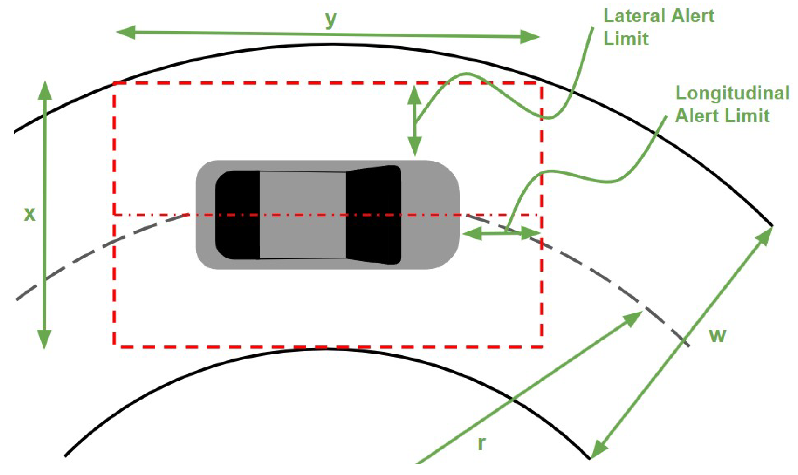
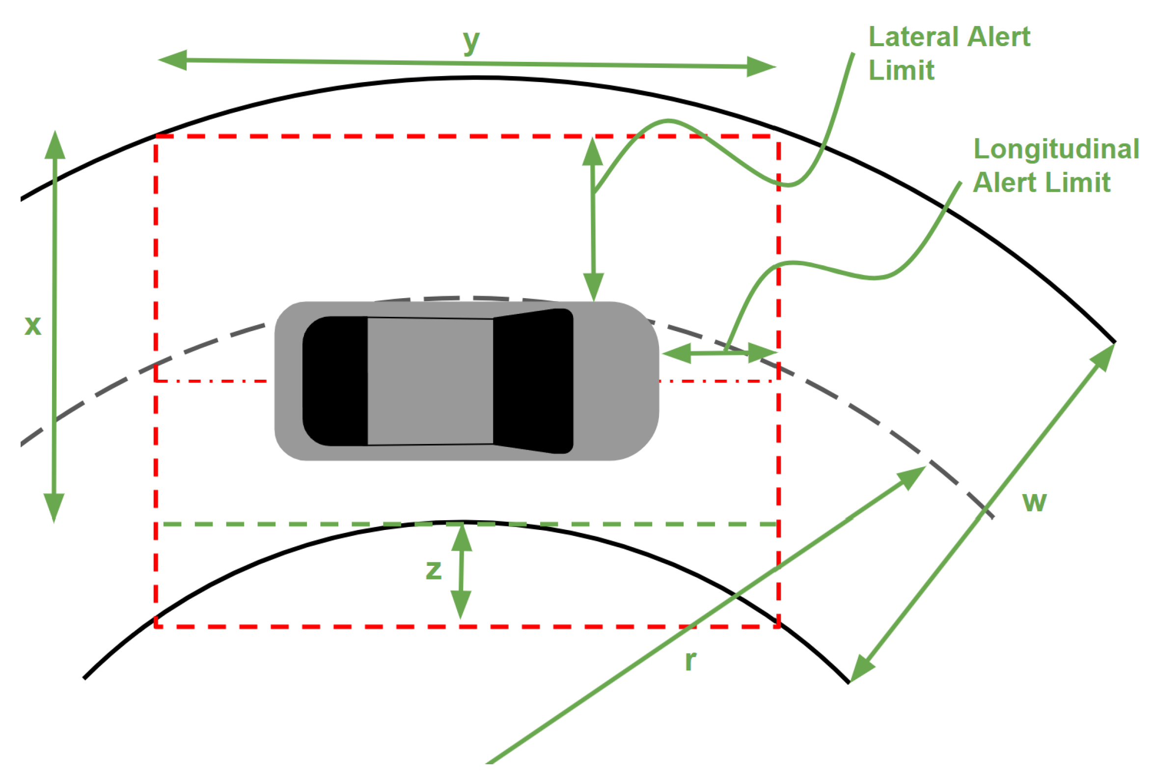
• An ideal trajectory is a trajectory that traverses the virtual corridor, thereby guaranteeing that the current driving task is accomplished collision-free.
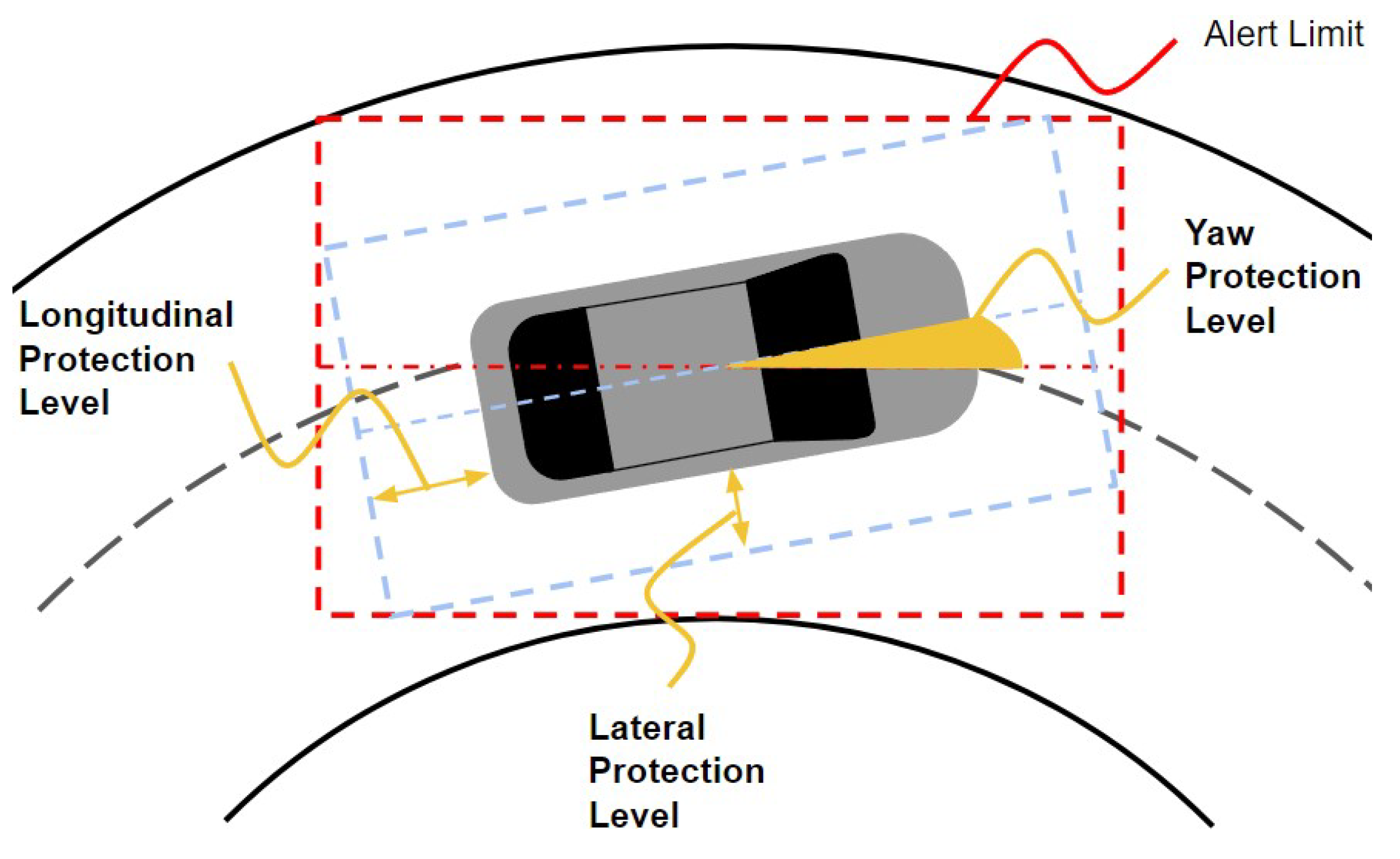
• A planner failure is when any of the lateral, longitudinal, or yaw trajectory errors, $e_{traj,\ast }$, (where ∗ is used to represent $lat$, $lon$, and $\psi$) exceed their corresponding thresholds: ${ϵ}_{traj,\ast }$. The trajectory error is the difference between the generated trajectory and the ideal trajectory. Under a zero mean, the Gaussian assumption is the following: $e_{traj,\ast }\sim \mathcal{N}(0,$${\sigma }_{traj,\ast }$²).
• A pose failure is when any of the pose errors, $e_{pose,\ast }$, exceed their corresponding thresholds: ${ϵ}_{pose,\ast }$. The pose error is the difference between where the VDS believes the ego vehicle is and where the ego vehicle truly is in the world. Under a zero mean, the Gaussian assumption is the following: $e_{pose,\ast }\sim \mathcal{N}(0,$${\sigma }_{pose,\ast }$²).
• A control failure is when any of the control errors, $e_{ctrl,\ast }$, exceed their corresponding thresholds ${ϵ}_{ctrl,\ast }$. The control error is the difference between the generated trajectory and where the VDS believes the ego vehicle is in the world. Under a Gaussian assumption, it is the following: $e_{ctrl,\ast }\sim \mathcal{N}(0,$${\sigma }_{ctrl,\ast }$²).

Before continuing with combining the risk allocation and protection levels, we should digress a little on the above definitions. The definition of $e_{ctrl,\ast }$ allows for its direct measurement. Both the generated trajectory and the estimated pose are available to the controller. Therefore, these quantities can be monitored online.

The definition of $e_{pose,\ast }$ does not share this property because it is computed based on where the ego vehicle truly is (referred to as the ground truth from now on). Without access to the ground truth, $e_{pose,\ast }$ cannot be measured.

Finally, the definition of $e_{traj,\ast }$ depends on the ideal trajectory definition and the virtual corridor definition by extension. Recall that the virtual corridor is specified similar to that of a lane and has a direct impact on the protection levels. Therefore, the planner’s task is to estimate the virtual corridor, with its predefined specifications (i.e., width, radius of curvature, etc.). In the simplest form, this may be simply identifying the unoccupied space available to the ego vehicle. The next task that the planner must do is to supply a time parameterization of the virtual corridor to generate an estimation of the ideal trajectory. In other words, the virtual corridor is a collision-free space that permits the ideal trajectory.

These definitions propose a specific interpretation of the VDS tasks as a whole and constitute a break from the developments in [19]. The underlying logic for these specific definitions is that they cause the modules’ errors to be additive:

$$e_{vds,\ast }=e_{traj,\ast }+e_{pose,\ast }+e_{ctrl,\ast }$$

(7)

Applying the Gaussian assumptions, we have:

$${\sigma }_{vds,\ast }^2={\sigma }_{traj,\ast }^2+{\sigma }_{pose,\ast }^2+{\sigma }_{ctrl,\ast }^2$$

(8)

Now, using the Gaussian assumption, we interpret these probabilities as the probability that the value of the random variable (i.e., $e_{vds,\ast }$) is between a symmetric range of $\pm z\sigma$ (the ± is commonly dropped to simplify notation) about the distribution’s mean. z is the constant multiple of the distribution’s standard deviation and it called the z score. This z score can be computed using the inverse cumulative distribution function (i.e., norminv in MATLAB 2021b).

Before proceeding, we point out that the probabilities $P_{traj}$ , $P_{pose}$, and $P_{ctrl}$ are not formal probabilities, because they have associated units (they are nevertheless common in risk analysis [9,19]). The choice of units is important when computing the z score. For instance, the designed $P_{ctrl}$ of $2.17\times {10}^{-9}$ failures per kilometer corresponds to $5.98\sigma$. If we instead present this in failures per meter, the value would become $2.17\times {10}^{-12}$, thereby corresponding to $7.02\sigma$. The ISO 26262 quantifies risks in failures per hour (i.e., ASIL D is ${10}^{-8}$ failures per hour of operation). So, we convert failures per km to failures per hour using the minimum speed that airbags will deploy, which is 16 km/h [27] (this also done in [19]).

The probabilities of failures per hour for the VDS, planner, pose, and control Modules are now $9.936\times {10}^{-8}$, $5.472\times {10}^{-8}$, $9.936\times {10}^{-9}$, and $3.472\times {10}^{-8}$, respectively. The corresponding z scores are $5.33$, $5.44$, $5.73$, and $5.52$ for the VDS, planner, pose, and control modules, respectively. These z scores then relate the protection levels to their corresponding standard deviations and thresholds:

$$\begin{array}{cc}\hfill \pm 5.33{\sigma }_{vds,\ast }& =\pm {\delta }_{\ast }\hfill \\ \hfill \pm 5.44{\sigma }_{traj,\ast }& =\pm {ϵ}_{traj,\ast }\hfill \\ \hfill \pm 5.73{\sigma }_{pose,\ast }& =\pm {ϵ}_{pose,\ast }\hfill \\ \hfill \pm 5.52{\sigma }_{ctrl,\ast }& =\pm {ϵ}_{ctrl,\ast }\hfill \end{array}$$

(9)

where ${\delta }_{\ast }$ represents the lateral, longitudinal, and yaw protection levels introduced in Section 2.1: ${\delta }_{lat}$ , ${\delta }_{lon}$ , and ${\delta }_{\psi }$ , respectively.

Now, we substitute (9) into (8) to obtain the following:

$${\left(\frac{{\delta }_{\ast }}{5.33}\right)}^2={\left(\frac{{ϵ}_{traj,\ast }}{5.44}\right)}^2+{\left(\frac{{ϵ}_{pose,\ast }}{5.73}\right)}^2+{\left(\frac{{ϵ}_{ctrl,\ast }}{5.52}\right)}^2$$

(10)

Equation (10) shows that the required error threshold for the planner, pose, and control modules cannot be designed independently. Control performance metrics are commonly specified as the traditional maximum lateral position from the lane’s width [15,16,17,18]. However, these definitions neglect the localization error and the trajectory error, which can lead to falsely believing that the VDS is safe.

Returning to the example with the 2019 Jeep Cherokee, we can use the same parameters used to compute the values in Table 2 to generate a surface plot of (10). The resulting surfaces are shown in Figure 6.

The engineer may now choose a point on these surfaces to design the thresholds. When verifying that the module performance meets the desired thresholds, the engineer must acknowledge that these selected thresholds are not deterministic maximum limits. Instead, they describe a distribution at the module’s selected risk allocation. Therefore, the engineer may prefer to present the surfaces from Figure 6 as standard deviations or at the corresponding 95 % probability levels rather than the designed probability threshold.

To illustrate how these specifications can be used to verify that requirements are met, we will perform a simple numerical example where the data from independent tests of each module are modeled with a zero mean Gaussian distribution. We proceed only with the Jeep Cherokee on an arterial road. To simplify this example, only the lateral component will be considered (although the other directions follow the same procedure). The lateral error thresholds will be set at 0.15 m, 0.31 m, and 0.38 m for the pose, control, and planner modules, respectively, by selecting a point on the lateral plot of Figure 6. This selection is arbitrary and should be considered tunable to balance the relative performances of the planner, pose, and control module.

To simulate independent experiments of each module’s lateral errors, 100,000 samples were taken from a normal distribution characterized by the module’s standard deviations computed using (9). These samples were then summed together to compute the experimental distribution of the VDS’s lateral position. Separately, the probability density function was computed for each module’s distribution, as well as the expected VDS distribution. Figure 7 shows that the histograms of the distributions fit perfectly with the expected probability density functions. The subfigure shows this more clearly for the VDS. This fit demonstrates the validity of Equations (8)–(10).

The method developed in this section to compute error thresholds can also be applied to modules upstream of the planner and pose modules such as the perception module. However, the errors need to be defined such that they permit an integration with planner, pose, and control errors. This is not trivial. For instance, it is not so obvious how errors should be defined for the map and perception outputs.

3. Results

3.1. A Case Study Showing Feasibility

The previous sections developed a new method of simultaneously allocating risk to the planner, pose, and control modules of a VDS. In this section, a case study from the literature is used to demonstrate (1) that this method is feasible, and (2) how to apply this method when there are data to support trade-off decisions. Refs. [14,28,29] developed new lateral controllers and validated them on an articulated bus. The bus was 18.3 m long and 2.6 m wide. Its pose module used DGPS, INS, and magnetic markers embedded in the road to provide positional feedback to the steering controller. There was no planner module in the conventional sense, because the route that the bus travels is fixed. Instead, we consider the planner module as the manual installation of the magnetic rods embedded into the road to be detected by the sensors on the bus [30,31].

The bus drives on an 1.8 km portion of Eugene Oregon’s EmX bus route (1.8 km in each direction). During this stretch, the bus operates in a special lane for most of the distance. This lane is mostly separated from traffic by curbs, but not continuously for the full route [32]. The route encompasses various “S”-shaped curves where the smallest radius of curvature is 26 m. The speeds at these curvatures are in the range of 6–12 m/s. The lane width ranges between 3 and 33 m [32].

The automatically steered buses operated for eight months and drove approximately 24,140 km (15,000 miles) (estimated from publicly available bus timetables [33]). Refs. [14,28,29] suggest that at some points in this portion of the EmX route, the buses were driven manually. The exact amount of miles driven manually is unknown, so we assume that half (12,070 km or 7500 miles) were driven manually, and the other half were driven automatically.

The overall goal of automating the steering control of the bus was to prove that doing so was feasible, as well as to validate several new control and fault detection algorithms [14,28,29]. The previously assumed TLS is therefore overly conservative for this case study. Instead, we set the TLS equal to typical human driving performance (or two orders of magnitude smaller). The TLS for this case study was therefore assumed to be $1.24\times {10}^{-8}$ fatal crashes per kilometer. This is further supported by the claim in [28] that the control system is at most an ASIL B system, and no formal methods are used to verify that the designed system meets its specifications.

Defining the vehicle length for this risk allocation is not obvious, because the center joint of the articulated bus allows it to bend around corners. To account for this, the largest wheelbase will be used instead of the length of the bus. The front wheelbase is 5.8 m and the rear wheelbase is 7.7 m (these do not add up to the overall vehicle length because the vehicle has front and rear overhangs). Therefore, the modified dimensions of the vehicle are 7.7 m long and 2.6 m wide. The wheelbase is also best modeled by a rectangle rather than a rectangle with rounded corners. Refs. [14,28,29] claim that the lane is so narrow and the curves are so sharp at times that the bus must be steered towards the inner curve to prevent the rear wheels from hitting the curbs. This indicates that the alert limit is not the vehicle’s edge but rather the tires during the largest curvature portions of the route. To account for this, the alert limit can be modified to allow the center portion of the vehicle’s body to leave the lane. This modified alert limit is shown in Figure 8.

The difference between Figure 2 and Figure 8 is that the lateral alert limit has increased by the quantity z. To derive a relationship between z and the other variables the Pythagorean theorem can be used:

$${(r-\frac{w}{2})}^2={\left(\frac{y}{2}\right)}^2+{(r-\frac{w}{2}-z)}^2$$

(11)

which can then be solved for z:

$$z=r-\frac{w}{2}-\sqrt{{(r-\frac{w}{2})}^2-{\left(\frac{y}{2}\right)}^2}$$

(12)

However, y in this equation cannot be greater than the wheelbase of the vehicle. So, we substitute $l_v$ for y and add this term to x in (2):

$$A{L}_{lat}=\frac{(x+z-w_v)}{2}$$

(13)

To compute the alert limits, three road specifications will be considered: arterial, collector, and an EmX bus lane. The EmX bus lane is defined to have a minimum radius of 26 m and a width of 3.0 m. Only the EmX bus lane will use (13) to compute the alert limits, since it contains the lowest minimum radius specification. The alert limits are shown in Figure 9.

To compute the protection levels, the speed will be used to motivate the selected yaw protection level. The arterial road has the highest design speed (50–100 km/h) and should have the largest yaw protection level [19]. The EmX road has the lowest design speed (0–43.2 km/h) and should have the smallest yaw protection level. A reasonable choice is therefore 0.03 rad (1.5 deg), 0.009 rad (0.5 deg), and 0.007 rad (0.4 deg) for the arterial, collector, and EmX roads, respectively. These values are used to compute the design curves for the lateral and longitudinal protection levels. The selected values are summarized in

Table 3. Protection levels and associated alert limits for EmX bus.

Road	${\mathit{\delta }}_{\mathit{lat}}$ [m]	${\mathit{\delta }}_{\mathit{lon}}$ [m]	${\mathit{\delta }}_{\mathit{\psi }}$ [rad] (deg)	${\mathit{AL}}_{\mathit{lat}}$ [m]	${\mathit{AL}}_{\mathit{lon}}$ [m]
Arterial	0.180	0.300	0.03 (1.5)	0.29	0.34
Collector	0.110	0.126	0.009 (0.5)	0.14	0.14
EmX	0.163	0.322	0.007 (0.4)	0.19	0.33

.

The protection levels are far more stringent than the ones presented in Table 2. Refs. [14,28,29] do not provide longitudinal tracking data, so the rest of this case study will focus only on the lateral components.

Using data collected from 8 months of operation, the automated steering system achieved a lateral error standard deviation of 7.15 cm and a zero mean. The manually steered vehicles had a lateral error standard deviation of 16.81 cm. Comparing these performance outcomes with the largest lateral protection levels for each road type suggests that the manually steered bus commonly placed the wheelbase outside the lane on collector roads. This reinforces the argument made in Section 2.2 that there should be an additional ratio to convert failures (lane departures) per mile into collisions per mile.

To compute this ratio, we begin by approximating the number of lane departures that occurred during operation. Since this data are not made available in [14,28,29] we will approximate it from publicly available crash data for Eugene, Oregon and the lateral steering performance. First, we will estimate the number of lane departures that are observed in the manually steered data. We begin by making the conservative assumption that all miles are collected on arterial roads. Then, using the Gaussian model for the lateral tracking performance, the range ± 18 cm can be shown to contain 71.57% of the observations (this can be computed using MATLAB’s normcdf). In other words, 71.57% of the miles driven manually do not contain a lane departure. Therefore, for the 7500 miles driven manually over the duration of eight months, there are approximately 2130 lane departures.

Since [14,28,29] do not mention any collisions, and there is no public crash data for those months of operation [34], it is assumed that no collisions occurred. As a result, the articulated bus’ estimated $P_{LD:C}$ is greater than 1:2130. If we use the 71.57% probability to extrapolate with more data, we can provide a better estimate of the $P_{LD:C}$ . According to [34], there were 13 collisions (no fatalities) in the location of interest on the EmX route between the years 2008 and 2021. None were attributed to vehicle system failures. During this period, approximately 302,000 miles were driven (also estimated from timetable data [33]). Using 302,000 miles driven manually instead of 7500, there were approximately 86,000 lane departures between the years 2008 and 2021. Therefore, a more accurate ratio would be 86,000 lane departures per 13 collisions (or approximately 6600 lane departures per collision).

Using these values in (6) and solving for $P_{vds}$ , we have:

$$\begin{array}{cc}\hfill 1.24\times {10}^{-8}& =(6.21\times {10}^{-9}+P_{vds})\left(\frac{1}{6600}\right)\left({10}^{-2}\right)\hfill \\ \hfill P_{vds}& =8.18\times {10}^{-3}\mathrm{Failures}/\mathrm{km}=0.1308\mathrm{Failures}/\mathrm{hr}\hfill \end{array}$$

(14)

Using the inverse cumulative distribution function, this probability corresponds to $1.51\sigma$ and can now be used to convert the protection levels into the VDS standard deviation, ${\sigma }_{vds}$, using (9). Solving (9) results in ${\sigma }_{vds,lat}=0.119$ m, $0.071$ m, and $0.108$ m for arterial, collector, and EmX roads, respectively. Since [14,28,29] present performances as standard deviations, (8) will be used rather than (10) to compute ${\sigma }_{ctrl,lat}$.

Solving (8) requires the standard deviations of the planner and pose modules. This information can be extracted from the description of the VDS reference path system in [30] and from the VDS position estimation system in [31]. The reference path is a series of magnets embedded into the road within 15 mm of the road center line [30]. How reliably this was done is unknown, so we assume this is given with 95 % confidence ($1.96\sigma$). Therefore, ${\sigma }_{traj,lat}=0.0076$ m. The magnetic reference system allows the VDS to localize itself within 5 mm to 3 cm of the ground truth [31]. We take the larger end of the range and again assume it is given with 95 % confidence ($1.96\sigma$). The pose module’s performance is therefore set at ${\sigma }_{pose,lat}=0.0153$ m. Substituting these values into (8) results in ${\sigma }_{ctrl,lat}$ 0.118 m, 0.069 m, and 0.107 m for the arterial, collector, and EmX roads, respectively.

3.2. Discussion

Comparing these target standard deviations with the experimental standard deviation for the automated steering system (${\sigma }_{ctrl,lat}=0.0715$ m) shows that the target level of safety was met for both the arterial and EmX roads, but not for the collector roads. In other words, the automated steering system developed in [14,28,29] is argued to be as safe as human drivers in the United States when the system is operated on arterial and EmX roads. However, when operated on collector roads, this automated steering system does not yet achieve this level of safety.

Nevertheless, two of the three lateral control performance requirements were satisfied by the steering controller developed in [14,28,29]. The lack of collisions during the duration of operation serves as empirical evidence of the feasibility of this methodology. Furthermore, the collector road requirement was very close to the controller’s performance, thus suggesting that the requirement is still achievable.

However, the following question is easily raised: why are there no recorded collisions on collector-type roads during the eight months of testing? The answer is that there simply were not enough driving data to observe a collision. The assumed TLS of $1.24\times {10}^{-8}$ fatal crashes per hour, or $1.24\times {10}^{-6}$ collisions per hour, predicts that no collisions should be observed during the 12,000 km of automatic steering operation.

Furthermore, public driving does not necessarily constitute sufficient validation of an ADS [11]. The result is that it is difficult to make confident claims that the steering controller is valid when the testing is based on public road driving. Unfortunately, this extends to using this case study to prove this methodology’s feasibility. Therefore, the reader is cautioned against relying on this method without using other systems engineering best practices such as the ISO 26262 and DIS 21448.

Finally, the benefits of this method are made more clear when contrasted with the proposed requirements used in [28]. In [28], the lateral control performance requirements were set as a standard deviation derived from an unspecified risk assumption and the ADS geometry of the bus on a straight road. By contrast, the method proposed in this paper accounts for (1) road curvature, (2) planner errors, (3) pose errors, and (4) control errors. It also provides a framework to develop fault-tolerant systems that can be directly linked to the TLS. This method is therefore more comprehensive than the one used in [28], and it provides a more robust method of deriving performance requirements.

4. Conclusions

This paper begins with a brief introduction on alert limits and protection levels in Section 2.1. In the same section, a rectangular model of passenger vehicles is used to compute the protection levels for various vehicle classes. The next section follows [19] partially. Two major differences are argued: (1) there should be an additional conversion factor between lane departures per mile and collisions per mile, and (2) the protection levels should be applied to the VDS rather than to the localization module. By imposing the protection levels on the VDS, definitions of failure can be set for each module such that their errors are additive. This allows for a simple approach to simultaneously allocate risk to the three modules.

In Section 3.1, an articulated bus performing lane keeping in a narrow lane has been used to demonstrate this method’s feasibility. This case study further demonstrates the risk allocation method developed in Section 2.1 and Section 2.2. It also provides data to support the argument that an additional conversion factor should be used in computing the target level of safety.

Finally, the case study in Section 3.1 demonstrates that this method is realistic in application. This verification shows that the system developed in [14,28,29] satisfies the requirements for arterial and EmX roads, but not for collector roads. Furthermore, our method suggests that had the ADS developed in [14,28,29] continued to operate on arterial and EmX, it would have achieved the target level of safety. However, the case study in question did not disclose enough data to make this claim more concrete.

References

1. On-Road Automated Driving (ORAD) Committee. Taxonomy and Definitions for Terms Related to Driving Automation Systems for On-Road Motor Vehicles; SAE International: Warrendale, PA, USA, 2021. [Google Scholar] [CrossRef]
2. Vidano, T.; Assadian, F.; Gulati, N. Artificially Intelligent Active Safety Systems. In AI-Enabled Technologies for Autonomous and Connected Vehicles; Murphey, Y.L., Kolmanovsky, I., Watta, P., Eds.; Springer International Publishing: Cham, Switzerland, 2023; pp. 213–254. [Google Scholar] [CrossRef]
3. Favaro, F.; Fraade-Blanar, L.; Schnelle, S.; Victor, T.; Peña, M.; Engstrom, J.; Scanlon, J.; Kusano, K.; Smith, D. Building a Credible Case for Safety: Waymo’s Approach for the Determination of Absence of Unreasonable Risk. arXiv 2023, arXiv:2306.01917. [Google Scholar]
4. Cruise. Cruise Safety Report; Technical Report; Cruise: San Francisco, CA, USA, 2022. [Google Scholar]
5. Hirshorn, S.R.; Voss, L.D.; Bromley, L.K. Nasa Systems Engineering Handbook; Technical Report; NASA: Washington, DC, USA, 2017. [Google Scholar]
6. Giusto, P.; Ramesh, S.; Sudhakaran, M. Modeling and analysis of automotive systems: Current approaches and future trends. In Proceedings of the 2016 4th International Conference on Model-Driven Engineering and Software Development (MODELSWARD), Rome, Italy, 19–21 February 2016; pp. 704–710. [Google Scholar]
7. Ioannou, P.A. (Ed.) Automated Highway Systems; Springer: New York, NY, USA, 1997. [Google Scholar]
8. ISO/DIS 21448; Road Vehicles—Safety of the Intended Functionality. International Organization for Standardization: Geneva, Switzerland, 2019.
9. ISO 26262; Road vehicles—Functional safety. International Organization for Standardization: Geneva, Switzerland, 2018.
10. de Gelder, E.; Elrofai, H.; Saberi, A.K.; Paardekooper, J.P.; Op den Camp, O.; de Schutter, B. Risk Quantification for Automated Driving Systems in Real-World Driving Scenarios. IEEE Access 2021, 9, 168953–168970. [Google Scholar] [CrossRef]
11. Khastgir, S.; Brewerton, S.; Thomas, J.; Jennings, P. Systems Approach to Creating Test Scenarios for Automated Driving Systems. Reliab. Eng. Syst. Saf. 2021, 215, 107610. [Google Scholar] [CrossRef]
12. Martin, H.; Tschabuschnig, K.; Bridal, O.; Watzenig, D. Functional Safety of Automated Driving Systems: Does ISO 26262 Meet the Challenges? In Automated Driving: Safer and More Efficient Future Driving; Springer International Publishing: Cham, Switzerland, 2017; pp. 387–416. [Google Scholar] [CrossRef]
13. Guldner, J.; Tan, H.S.; Patwardhan, S. Study of design directions for lateral vehicle control. In Proceedings of the 36th IEEE Conference on Decision and Control, San Diego, CA, USA, 12 December 1997; Volume 5, pp. 4732–4737. [Google Scholar] [CrossRef]
14. Tan, H.S.; Huang, J. Design of a High-Performance Automatic Steering Controller for Bus Revenue Service Based on How Drivers Steer. IEEE Trans. Robot. 2014, 30, 1137–1147. [Google Scholar] [CrossRef]
15. Rokonuzzaman, M.; Mohajer, N.; Nahavandi, S.; Mohamed, S. Review and performance evaluation of path tracking controllers of autonomous vehicles. IET Intell. Transp. Syst. 2021, 15, 646–670. [Google Scholar] [CrossRef]
16. Snider, J.M. Automatic Steering Methods for Autonomous Automobile Path Tracking; Technical Report; Robotics Institute, Carnegie Mellon University: Pittsburgh, PA, USA, 2009. [Google Scholar]
17. Hoffmann, G.M.; Tomlin, C.J.; Montemerlo, M.; Thrun, S. Autonomous Automobile Trajectory Tracking for Off-Road Driving: Controller Design, Experimental Validation and Racing. In Proceedings of the 2007 American Control Conference, New York, NY, USA, 9–13 July 2007; pp. 2296–2301. [Google Scholar] [CrossRef]
18. Spielberg, N.A.; Brown, M.; Kapania, N.R.; Kegelman, J.C.; Gerdes, J.C. Neural network vehicle models for high-performance automated driving. Sci. Robot. 2019, 4, eaaw1975. [Google Scholar] [CrossRef] [PubMed]
19. Reid, T.G.; Houts, S.E.; Cammarata, R.; Mills, G.; Agarwal, S.; Vora, A.; Pandey, G. Localization Requirements for Autonomous Vehicles. SAE Int. J. Connect. Autom. Veh. 2019, 2, 173–190. [Google Scholar] [CrossRef]
20. Development of Satellite Navigation for Aviation Technical Description of Project and Results; Technical Report; Stanford University: Stanford, CA, USA, 2009.
21. Feng, Y.; Wang, C.; Karl, C. Determination of Required Positioning Integrity Parameters for Design of Vehicle Safety Applications. In Proceedings of the 2018 International Technical Meeting of The Institute of Navigation, Reston, VA, USA, 1–29 January 2018; pp. 129–141. [Google Scholar]
22. Kigotho, O.N.; Rife, J.H. Comparison of Rectangular and Elliptical Alert Limits for Lane-Keeping Applications. In Proceedings of the 34th International Technical Meeting of the Satellite Division of The Institute of Navigation (ION GNSS+ 2021), St. Louis, MO, USA, 20–24 September 2021; pp. 93–104. [Google Scholar]
23. Cicchino, J.B. Effects of lane departure warning on police-reported crash rates. J. Saf. Res. 2018, 66, 61–70. [Google Scholar] [CrossRef] [PubMed]
24. Schafer, H.; Santana, E.; Haden, A.; Biasini, R. A Commute in Data: The comma2k19 Dataset. arXiv 2018, arXiv:1812.05752. [Google Scholar]
25. Kapania, N.R.; Gerdes, J.C. Design of a feedback-feedforward steering controller for accurate path tracking and stability at the limits of handling. Veh. Syst. Dyn. 2015, 53, 1687–1704. [Google Scholar] [CrossRef]
26. Blanch, J.; Walter, T.; Enge, P. Protection level calculation using measurement residuals: Theory and results. In Proceedings of the 18th International Technical Meeting of the Satellite Division of The Institute of Navigation (ION GNSS 2005), Long Beach, CA, USA, 13–16 September 2005; pp. 2288–2296. [Google Scholar]
27. Wood, M.; Earnhart, N.; Kennett, K. Airbag deployment thresholds from analysis of the NASS EDR database. SAE Int. J. Passeng. Cars-Electron. Electr. Syst. 2014, 7, 230–245. [Google Scholar] [CrossRef]
28. Huang, J.; Tan, H.S. Control System Design of an Automated Bus in Revenue Service. IEEE Trans. Intell. Transp. Syst. 2016, 17, 2868–2878. [Google Scholar] [CrossRef]
29. Huang, J.; Tan, H.S. Development and Validation of an Automated Steering Control System for Bus Revenue Service. IEEE Trans. Autom. Sci. Eng. 2016, 13, 227–237. [Google Scholar] [CrossRef]
30. Chan, C.Y.; Tan, H.S. Evaluation of Magnetic Markers as a Position Reference System for Ground Vehicle Guidance and Control; Technical Report; California Path Program, Institute of Transportation Studies: Berkeley, CA, USA, 2003. [Google Scholar]
31. Chan, C.Y.; Bougler, B.; Nelson, D.; Kretz, P.; Tan, H.S.; Zhang, W.B. Characterization of magnetic tape and magnetic markers as a position sensing system for vehicle guidance and control. In Proceedings of the 2000 American Control Conference. ACC (IEEE Cat. No.00CH36334), Chicago, IL, USA, 28–30 June 2000; Volume 1, pp. 95–99. [Google Scholar] [CrossRef]
32. Thole, C.; Cain, A.; Flynn, J. The EmX Franklin Corridor BRT Project Evaluation; Technical Report; National Bus Rapid Transit Institute: Los Angeles, CA, USA, 2009. [Google Scholar]
33. EmX Map and Schedule. Available online: https://www.ltd.org/system-map/route_103/ (accessed on 17 August 2023).
34. All Motor Vehicle Crashes 2007–2021. Available online: https://www.lcog.org/thempo/page/advanced-user-data (accessed on 17 August 2023).
Figure 1. A generic ADS architecture separating the VDS and vehicle system.
Electronics 13 00902 g001
Figure 2. Lateral and longitudinal alert limits.
Electronics 13 00902 g002
Figure 3. The protection levels depicted as a rotated rectangle within the alert limit.
Electronics 13 00902 g003
Figure 4. The trade-off curves between the lateral alert limit and the longitudinal alert limit for a Jeep Cherokee.
Electronics 13 00902 g004
Figure 5. Protection levels of a 2019 Jeep Cherokee.
Electronics 13 00902 g005
Figure 6. The ellipsoid-like surfaces showing the trade-off between planner, pose, and control module thresholds.
Electronics 13 00902 g006
Figure 7. The probability density of the pose, control, trajectory, and virtual driver system lateral errors.
Electronics 13 00902 g007
Figure 8. Modified alert limit for EmX bus on high-curvature portions of route.
Electronics 13 00902 g008
Figure 9. Alert limits for the EmX bus.
Electronics 13 00902 g009