Abstract
Query-time Exploratory Data Analysis (qEDA) is an increasingly demanding aspect of the data analysis process that entails visually and quantitatively summarizing, comprehending, and interpreting the primary characteristics of a dataset. Nowadays, an imperative procedure is popular in relational databases for EDA because it enables us to write multiple dependent declarative queries with imperative logic. As online analytical processing (OLAP) systems contain extremely large datasets, data scientists often need quick visualizations of data, using approximate processing of imperative procedures, before analyzing them in their entirety. We identify gaps in the existing techniques, in that they are unable to sample both declarative-dependent statements and control logic at the same time and perform multi-dependent sampling-based approximate processing within the permitted time in qEDA. Traditional approximate query processing (AQP) involves tuple sampling for a single query approximation and enables queries to be executed over arbitrary random samples of tables. However, available AQP methods cannot produce a further representative sample of the data distribution for the dependent statements to estimate accurately and quickly for multiple dependent statements. On the other hand, sampling control structures, like loops and conditional statements, are discussed separately, without regard to the imperative structure of statements in a procedure. In this study, we propose Forester, a novel agile approximate processing method for imperative procedures that performs imperative program-aware sampling, which includes both statements with control regions (i.e., branch and loop) and processes them approximately within the permitted time in qEDA. Our method produces more targeted samples for each relation, while maintaining the data and control flow of dependent queries and imperative logic and determining all the conditions for a relation across all the statements in the sample that guarantee the existence of relevant data for dependent data distribution. Utilizing a workload of multi-statement imperative procedures from the Transaction Processing Performance Council Decision Support (TPC-DS) database, our experiment demonstrates that Forester outperforms the existing system in sampling, producing minimum error, and improving response time.
1. Introduction
An imperative procedure that employs the imperative programming paradigm is a collection of SQL statements stored in a database and executed as a unit. In contrast to a declarative stored procedure, which focuses on describing what must be done without specifying the exact steps, an imperative stored procedure specifies the exact order of operations required to accomplish a specific result. Relational database management systems (RDBMS) like Oracle, SAP Hana, Microsoft SQL Server, MySQL, and PostgreSQL typically contain imperative stored procedures. These procedures may contain IF-THEN statements, iterations, variable assignments, and other imperative logic structures. They are frequently employed for complex data manipulations, transaction administration, and the deployment of business logic within a database.
Exploratory data analysis (EDA) is a data analysis process that involves understanding, analyzing, and summarizing a dataset’s main features, both numerically and visually. The practice of using queries to perform exploratory analysis on a dataset in real-time is known as query-time exploratory data analysis [1]. This entails interactively examining the data and obtaining knowledge by instantly querying the dataset. It encompasses several processes such as interactive queries, aggregate and summary statistics, data distribution analysis, correlation analysis, quality assessment of the data, and iterative exploration.
Approximate processing estimates query responses by analyzing a sample of the data rather than the complete dataset. This is beneficial for complex queries with enormous datasets that would otherwise take a long time and a lot of resources. Sample-based approximate processing is ideal for situations where imprecise results are acceptable because it trades accuracy for speed. Query-time exploratory data exploration, visualization, and dashboard applications employ it for real-time or near-real-time answers. It executes queries faster but sacrifices accuracy. The sample size, representativeness, data, and query processing affect the estimate’s quality.
An imperative program-aware approximate processing problem is more critical than declarative approximate processing. It integrates two major problems: (i) sampling for an imperative procedure should be aware of imperative structures, such as statement dependencies and control logic, for greater accuracy, and (ii) approximate processing should be aware of faster processing in query time, when rewriting the procedure, to process it on the generated sample.
Data sampling and control logic sampling for approximate query processing (AQP) have been the two separate subjects of a great deal of research. AQP research, especially in two-stage and adaptive sampling [2,3,4] that deals with sampling from previous sampling, is similar to sampling for imperative program-aware data sampling. However, they cannot solve certain issues such as data synchronization, parameter effects, dependent sampling criteria, control logic sampling, etc. On the other hand, research in control logic sampling [5] (i.e., sampling loops and branches) does not deal with data sampling for imperative procedures.
Using an intuitive example in Figure 1, we demonstrate the problem in the approximate processing of an imperative procedure. The figure shows a control flow diagram (CFG) of an imperative procedure, where we denote statements as . Directed lines between statements define the dependencies between statements. Statement contains imperative loop logic. Statements , , and consume data directly from base tables , , , and . If we sample for a procedure using the current available methods, we are only able to sample tuples regarding a base table for a single query. We show these possible samples for a procedure using dashed, directed lines.
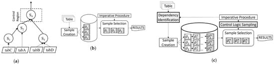
Figure 1.
Comparative evaluation for approximate processing of an imperative procedure. (a) Control flow graph of a procedure. (b) Traditional approximate processing. (c) Proposed approximate processing.
We identify the following limitations of this sample for the approximate processing of an imperative procedure: (i) depends on and . If statement contains a condition, sampling from statements and may not contain tuples that are representative. (ii) We cannot sample dependent statements. For instance, sampling an additional statement has no effect. It means that we continue to rely on , , and samples for the approximate processing of . (iii) Imperative logic can be positioned anywhere in the CFG that is dependent on the previous query result (for example, in branches or an iterative or recursive loop). However, we cannot sample where we can contemplate imperative logic. Finally, (iv) we can sample a table in a query that consumes from a base table individually. However, a procedure may comprise a large number of base tables and dependent statements. Sampling for an entire procedure is missing from the current available techniques.
In this study, we identify a novel problem called query-time exploratory data analysis that utilizes the approximate processing of an imperative procedure. It integrates two major problems: (i) imperative sampling, which generates imperative samples for an imperative procedure at query time to achieve accuracy as a combination of imperative data and control logic sampling problems, and (ii) imperative sample-aware rewriting of the procedure, which deals with rewriting the procedure with sampling effects to produce a faster processing time.
In order to solve the problem, we propose Forester, a novel method called agile approximate processing for the approximate processing of an imperative procedure in query-time data analysis. It represents the data and control logic of an imperative procedure, using Forest representation to gain insights into the imperative sampling problem. The Forester extracts forest data structure from the forest to provide solutions for imperative data sampling and a sampling control logic algebraization method to sample imperative control regions during the rewriting procedure.
Forester employs a novel multi-dependent data sampling method called multi-dependent layer (MDL) sampling, which utilizes the forest data structure for imperative data sampling. However, there is a technical challenge in imperative data sampling using the MDL sampling method. If an imperative procedure consists of a large number of dependent statements, the MDL sampling method creates multiple samples that are aware of each dependent statement to produce the final sampling at the root, which is referred to as the cold sampling-based approximate processing. This cold sampling-based method achieves higher accuracy. However, it may fail to produce a faster processing time in query-time EDA.
In order to handle this issue, Forester employs hot-sampling approximate processing, which analyzes the partial benefit of MDL sampling to produce faster processing times while performing cold sampling in the background. Forester utilizes valid cold sampling when it is available, instead of hot sampling. Cold sampling is not valid if the current state of the database changes. Forester is useful for precomputed sampling-based approximate processing by utilizing the cold sampling-based method. On the other hand, runtime sampling-based approximate processing can be called a synonym of query-time exploratory data analysis using approximate processing in this study.
Finally, we propose a sampling clause, FORESTSAMPLE, during the calling procedure, to determine the scale of the imperative sample size.
We summarize the contributions as follows:
- We propose Forester, a novel imperative program-aware sampling-based approximate processing technique for an imperative procedure. It utilizes a novel forest representation that includes both imperative data and the logic of a multi-statement procedure and extracts a forest data structure that represents the imperative data of multiple relations in a procedure.
- We identify multi-dependent sampling layers to determine imperative samples from imperative data and propose an algebraization method to sample control logic during the rewriting procedure.
- We propose a novel agile approximate processing method for imperative procedures that is aware of processing within query time in qEDA.
- We propose two novel imperative sampling methods in agile approximate processing, such as cold and hot sampling, to trade off between accuracy and speed for qEDA.
- We propose a novel sampling clause FORESTSAMPLE during the calling procedure, to determine the sampling scale.
We organize the remaining sections as follows. In Section 2 and Section 2.1, Section 2.2 and Section 2.3, we describe the novel concepts of this study: imperative sampling, imperative data sampling, imperative control logic sampling, and imperative procedure rewriting, respectively. In Section 3, we discuss the overview of Forester. After that, in Section 4, Section 6, Section 7 and Section 7.1, Section 7.2 and Section 7.3, we illustrate Forester for query-time approximate processing. In Section 9, we discuss the optimization process in Forester. Section 12 evaluates Forester by demonstrating experiments. We discuss the related literature in Section 13. We conclude our study in Section 15.
2. Imperative Sampling
Imperative sampling refers to a sampling method that identifies imperative samples from imperative data and executable control regions for approximate processing. We first illustrate an imperative procedure using Example 1 in Figure 2. Next, we define imperative data and an executable control region with proper illustrations in Figure 3. After that, we define imperative samples.
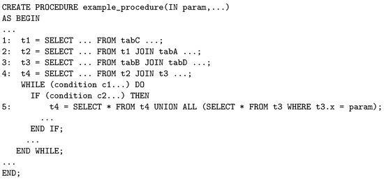
Figure 2.
Example 1: an imperative procedure.

Figure 3.
An imperative procedure with imperative data and executable control region.
Example 1 contains multiple imperative SQL statements (1, 2, 3, 4, and 5). We call these imperative SQL statements because they have producer–consumer relationships and are combined with variables. Statements 1, 2, 3, and 4 are producer statements of 2, 4, 4, and 5, respectively. Statements 1, 2, and 3 consume data directly from , , , and . Additionally, the procedure contains control regions that merge rows iteratively or gather the outcome of a branch in a table variable, .
The data that are manipulated or processed within the context of an imperative procedure are referred to as imperative data. They depend on dependent data distribution based on producer–consumer relationships between statements, parameters, local variables, or temporary storage. Suppose an imperative procedure contains two statements, and , with a producer–consumer relationship. Statement is a producer statement of Statement . and are the temporary storages (i.e., temporary tables or table variables) that store the intermediate results of and . Local variables, or parameters, affect both statements. Dependent data distribution flows from to , based on imperative logic. We call temporary storages and imperative data.
In Figure 3, we show that Statement contains the imperative data of , denoted by , because it evolves its consumer statements using . Similarly, and in statements and are also imperative data of , because they evolve their consumer in statements and , respectively. Similarly, we have other imperative data for , , and .
The executable control region that manipulates or processes executable data within the context of an imperative procedure is referred to as imperative control logic. In this study, we explicitly deal with loops and branches as imperative control logic. Let an imperative procedure contain a loop with condition and a branch with condition . We refer to the control logic as the statements in control regions based on and , respectively.
In Figure 3, we show that statement in the control region that is to be executed. We call it an executable control region. In the case of a branch, the executable control region follows the execution path to execute statements.
The problem is to identify samples for the dependent statements or control region that can more precisely estimate the characteristics of each subgroup of the population while obtaining accurate estimates of the parameters of the entire population. Nonetheless, it is essential to design the sampling process with care to ensure that the resulting estimates are impartial and reliable.
We define imperative samples as follows:
Imperative samples refer to sampled data with a sample of executable control regions for the approximate processing of an imperative procedure. Let N represent the original data or control logic, S represent an imperative sampled data or control logic, and the scale factor of sampling is f. Then, we represent the sampled data from a sample of control regions as follows:
An imperative sampling problem consists of two sampling problems: (i) imperative data sampling and (ii) imperative logic sampling. We now discuss these two problems.
2.1. Imperative Data Sampling
Imperative data sampling refers to a data sampling method that identifies imperative data samples from imperative data for approximate processing. We define imperative data samples as follows:
The imperative data sampling problem for the approximate processing of a procedure is how efficiently we can generate a representative sample from imperative data. Using the existing approximate query processing methods, we are able to generate samples for a procedure from a relation regarding a statement to a certain extent. We use a mixture of sampling and filtering. First, we select a random sample from the database and apply a filter to select only the data that fit the desired criteria. This method is useful when the user analyzes a subset of the data; however, the database is too large to pick a sample based on criteria. We represent a relational algebra of data sampling from a relation regarding a statement in the following Equation (2):
where R is the input relation, P is the row selection probability, and produces a randomly selected number between zero and one. Each row of the input relation is subjected to the selection condition , and only rows that meet this condition are added to the output relation or relational variable . This ensures random sampling by giving each row in the input relation an equal and distinct likelihood of selection. We use the clause to reduce the returned rows to k. This returns a maximum of k rows from that meet the random sampling condition .
We generate data samples for the procedure in the example utilizing Equation (2), and we are able to generate samples from the base tables regarding a statement. We demonstrate the relational algebra that represents the sampling for the approximate processing of the procedure in Figure 4.
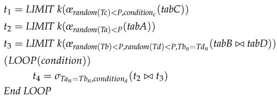
Figure 4.
Relational algebra for approximate processing of the procedure in the example.
We analyze the data sampling in Figure 4. We identify the following issues: (i) We are only able to create data samples for base relations such as , , , and regarding the first three statements. Sampling from relational variables and in a dependent statement has no effect if we intend to sample for and , because relational variables do not support sampling. If we materialize and , we are able to sample and . However, random sampling cannot guarantee the targeted representative sample after materialization for the statement with , because and are in a join relationship. As a result, some representative tuples from may not have any effect regarding joining with . (ii) The existing method considers the condition (it can be parameterized) of the first statement, , during sampling in . However, sampling in may not be representative, as its dependent statement with contains a condition, for . Finally, (iii) imperative logic depends on the samples in and . If the samples in and are not representative, it causes a serious performance drawback in executing imperative logic.
We cannot further sample for the base tables regarding dependent statements that are more targeted and representative using the existing sampling methods. If we reduce tuples for a base table from the second sample, we can generate a more targeted sample for the dependent statement. Moreover, these samples contain less data but have higher chances of being selected.
However, sampling with dependent statement criteria in a procedure has various challenges. One problem is choosing a sample size that is accurate and computationally feasible. Defining relevant sampling criteria is difficult and requires domain expertise to ensure the sample accurately represents the total flow of data. If we do not define the criteria or apply the sampling method properly, the selection of criteria may bias the sample. Finally, meeting the selection criteria while ensuring the sample is representative of the flow of data is difficult. As a result, we must carefully examine these issues to ensure an accurate and unbiased sample when sampling with dependent statement criteria.
2.2. Imperative Control Logic Sampling
Imperative control logic sampling refers to a logic sampling method that identifies a sample of executable control regions for data sampling from imperative control regions for approximate processing. We define imperative control logic samples as follows:
In an imperative program, an imperative control logic sample refers to a conditional structure that enables the program to perform various operations or apply particular logic based on specific sampling conditions, as well as a control flow structure that enables us to choose and process a subset of data from a larger dataset for analysis or manipulation.
In order to speed up processing while compromising some accuracy, loop sampling techniques for approximate processing include performing a selection of loop iterations selectively. The main objective of these methods is to conserve computational resources like time, energy, or memory bandwidth, and they are helpful when approximations of the results are acceptable. A number of loop sampling strategies, including threshold-based sampling, stridded sampling, random sampling, regular skipping, and so on, are available for approximate processing.
However, adapting loop sampling techniques for the approximate processing of an imperative procedure is not accurate in the case of multiple dependent statements with filter conditions, because some loops may not be relevant. For example, if the loop condition is dependent on a declarative statement and the sample of this statement is not targeted or focused, loop sampling samples the irrelevant subset of data. Thus, loop sampling for approximate processing cannot be accurate by simply adapting loop sampling; it must be followed by a focused sampling of the dependent statement.
Branch sampling has traditionally been employed in approximate query processing (AQP) to accelerate query execution by sampling and evaluating a subset of paths or branches in a query execution plan. Complex queries with multiple branches, for which evaluating each branch would be resource-intensive and unnecessary in order to acquire an approximation of the result, can benefit significantly from this method.
However, sampling a subset of branches is not accurate for the approximate processing of an imperative procedure, because branch sampling misses the dataset of relevant branches for the data distribution in dependent statements. Therefore, rather than sampling selective branches, it is important to estimate the potential contribution of the relevant branch to the final result based on the execution path.
2.3. Imperative Procedure Rewriting
Imperative procedure rewriting refers to the execution plan, which performs approximate processing that reflects imperative data and control region sampling. This problem reflects two sampling issues during procedure rewriting: (i) reflecting imperative data sampling: replace base relations with the sample name from imperative sampling; and (ii) reflecting imperative control logic sampling: rewrite the imperative logic conditions.
Suppose an imperative procedure contains imperative data from base table B and an imperative condition C. If we have an imperative data sample from B with an imperative logic sample from C, we rewrite the procedure by replacing B with and rewriting C with .
In current practice, procedure rewriting problems for approximate processing are limited to data source replacement, where a procedure uses sampled data instead of original data. However, it cannot deal with sampling imperative control logic with the same sampling scale. On the other hand, to support agile approximate processing, we need to identify the latest imperative sample of a base table to replace the original data source. However, the existing study cannot solve this.
3. Forester OverView
We propose Forester, a sample-based approximate processing technique for query-time exploratory data analysis. We named it Forester because it represents imperative data and control logic using a forest-like representation that consists of multiple trees. The notion is that a forester plucks parts of trees from the forest, which is similar to extracting an imperative sample from imperative data and control regions.
We illustrate the Forest in Figure 5. In the figure, the x-axis represents the trees from every relation in the procedure. For example, trees of , ,… in the procedure. The y-axis represents the imperative data of each relation in each statement, including control regions.
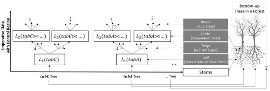
Figure 5.
Forest representation for sampling in Forester.
A forest represents the imperative data and control logic of an imperative procedure using multiple related trees. A tree refers to the imperative data and control region of a base table. We represent the imperative data and control region as the stem of a tree, where a stem consists of layers of limbs and twigs from root to leaf. An imperative datum evolves from base table to root by the imperative statements (i.e., a producer–consumer relationship), which are represented as layers of limbs of a tree. We represent control logic (i.e., loops and branches) as twigs attached to a limb. One interesting feature of this forest is the interdependence of some trees, which signifies that a given statement may incorporate multiple base tables or consumer statements. We represent the join between imperative data from multiple base tables as layers of limbs that are dependent on multiple stems.
Above is a real-life example of agile reporting, to illustrate our intention. A forester, in the context of this paragraph, refers to a real-life forest officer rather than the name of our proposed technique. Their responsibility is to report the condition of the forest to the authority at a given time. Their intention is to take a sample of leaves from representative limbs that are more representative to prepare the report. They apply an agile (incremental) reporting method based on time. They start taking leaves from the top, towards stems and through limbs, for their agile reporting. Plucking leaves from the top means they may not come from well-representative limbs; however, it is faster. If the forester comes closer to the stem, they find more representative limbs to pluck leaves; however, it takes more time. Thus, the forester is aware of the permitted time to conduct agile reporting and how much they are allowed to pluck the representative leaves to prepare the report.
Similar to this real-life agile reporting, the sampling of a base table may evolve through a series of dependent statements until it reaches the root. We need to identify a sample of base tables that are aware of the statement dependencies. Our algorithm utilizes agile approximate processing that uses hot sampling-based approximate processing in order to perform query-time exploratory data analysis, based on permitted time. If it finds a valid cold sampling, it utilizes the cold sampling-based approximate processing.
4. Forest Data Structure
Forest data structure refers to a data structure that consists of multiple tree data structures for imperative data sampling. We extract this data structure from the forest representation by separating layers of limbs from the stem of a tree. By employing a data flow graph, we construct a forest data structure that represents imperative data. We denote each layer of a limb in the forest data structure as a layer. A layer represents imperative data distribution from a producer statement to consumer statements.
A Forest of a procedure is a multiple tree structure, , where the following is true:
- N is a set of nodes that represent the data of a relation and control logic (i.e., roots, limbs, and leaves). Each node is labeled with , which corresponds to intermediate or final data, , of a relation, R, at the layer .
- E is a set of directed edges that represent the hierarchical relationships between the nodes. Each edge indicates the relationship between the two data sources.
Figure 6 shows how we extract forest data structure from the data flow graph of a procedure. Figure 6a shows the data flow diagram of a procedure. In Figure 6b, each box represents imperative data in a layer of a relation, where the directed lines show the dependency between two imperative data of the same relation.

Figure 6.
Forest data structure. (a) Data flow graph; (b) Four trees inside Forest.
The layer is the level at which imperative data for a base relation are generated from the stored data or previous data of the relation. In each layer, it represents the relational data of every table. We denote it with , where is relation-dependent level.
The total number of sampling layers, , depends on the level of dependency of a relation, called the relation-dependent level (RDL) of the relation. The RDL is the level of a relation at which imperative data from a base relation are used to process a statement within a procedure. We denote it with , where R is a relation. From the data flow graph of a procedure, we derive the RDL of a relation. The total number of RDLs corresponds to the number of levels where the relation used in a statement ascends from the base table to the root. We number the in such a way that imperative data at the same number layer can be processed in parallel. In Figure 6b, has three layers: , , and . Imperative data in all four relations at and can be processed in parallel.
Imperative data in a tree have two major parts: (i) Top Leaf: the original data of a base table. In Figure 6b, the data at the layer are the top leaves. (ii) Leaf at Layered Limb: imperative data after the base table to the root. In Figure 6b, the data at the layer are the leaves at layered limbs. Each imperative datum of a relation in the layer depends on one or multiple relational data in the layer, excluding the data in the first layer.
We use the data flow graphs of a procedure to construct a forest. A forest is a combination of multiple trees. Each tree is responsible for the imperative data, from the base table to the root statement. We demonstrate a forest using our running example in Figure 7. We achieve the forest of the example procedure using a data flow graph. In Figure 7, the forest is the combination of four sampling trees for , , , and , respectively.
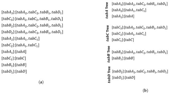
Figure 7.
Forest and tree construction; (a) Forest construction; (b) Tree construction.
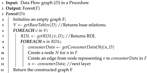
We provide a pseudocode for creating a forest graph of an imperative procedure in Algorithm 1. It initializes an empty graph F with the process. Initially, it generates a node N in the graph for every variable or data object () in the procedure that depends on base tables. After that, it iteratively looks for a series of consumer data objects, generating a node N in the graph for each variable or data object () in the process. In the event that data flows from variable V to variable , the process establishes an edge in F between the nodes representing V and . Finally, it returns graph F.
| Algorithm 1: Algorithm for Forest Construction. |
 |
5. MDL Sampling
MDL sampling refers to an imperative data sampling method that samples imperative data from their producers. It utilizes the forest data structure. MDL sampling creates a series of dependent sampling layers from the tree structure of each base table by utilizing sampling criteria.
5.1. Sampling Layer
Sampling layer refers to layers of forest data structure that are required for sampling. We identify which layer in the forest data structure is required for sampling or we use the sample from the previous layer. Suppose there are three layers, , , and , in the forest data structure. depends on , and depends on . We identify and layers that are required for sampling, and uses the sample from . We call and the sampling layers, and , where and are merged in . The imperative sampling of all relations at the same sampling layer must be performed in parallel, to produce the latest sample for the dependent sampling layers.
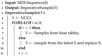
We identify the imperative samples of a relation at each layer to construct the MDL sampling from leaf to root of the forest data structure. MDL sampling has two major parts: (i) sampling fresh leaves, and (ii) sampling leaves in layered limbs.
We perform the sampling fresh leaves method in the first layer, , using a combination of a sampling technique and the criteria of the layer. We identify the samples of the first layer from base relations by combining the criteria of the first layer, , of each relation. We perform sampling leaves in the layered limb method at higher layers, . We identify the latest imperative samples of relations to generate a sample at higher layers, , using the criteria for each layer of a relation.
The goal of MDL sampling is to make the imperative samples more focused and targeted. We employ a sampling technique combined with criteria in the first layer to generate preliminary samples from the original base table. If we employ a sampling technique combined with criteria from the second layer, it generates a subset of the first layer sample that is more targeted; however, it reduces tuples based on the same scale factor. The problem is that if the number of layers is large, it generates a sample that contains a few (possibly zero) tuples at the higher layers. It creates inconsistencies with the imperative samples. Thus, we only utilize criteria to sample imperative data at higher layers, rather than combining a sampling technique with criteria. It guarantees the imperative samples are more targeted at the final layer.
Let P be an imperative procedure with X number of relations. Let represent relations containing tuples, and let represent a sample of size . We achieve the samples of relation at the and , with the criteria , using the following Equations (3) and (4), respectively:
where is the scale factor, f, used to adapt each relation’s sample result to the actual data.
We determine the requirement of sampling in a layer of forest data structure using an RDL degree. The RDL degree of a relation refers to the number of dependencies on other relations or relational variables at . We denote it with .
We determine the first sampling layer, , by determining , and sampling depends on a single base relation. We determine the higher sampling layers, , of a relation by identifying , where . It indicates that, except for , we do not generate a sample in an where 1, but instead use a sample from the previous layer, , of the relation. If we sample a higher layer where D(n) = 1, we sample the same relational data, which have no dependencies with another relation. It reduces the sample size; however, it loses some targeted data in higher sampling layers. Therefore, the total number of sampling layers, , in a relation equals the number of in a relation where plus one.
Figure 8 shows the sampling layers of four relations in an imperative procedure. is the generated sample for a relation in a RDL. It shows that , , , and have 3, 3, 2, and 2 sampling layers, respectively. We observe that samples from every relation are at , where . This indicates that, in the first layer, , we generate samples of every relation from the base tables. In the case of the second layer, of , we do not increase the sampling layers, , of the relation because it contains . It means that in the of , we use the sample of , of . In the remaining case from the second layer, we generate a new sample in every of a relation because it has . We provide the pseudocode for the MDL sampling in Algorithm 2.
| Algorithm 2: Algorithm for MDL Sampling. |
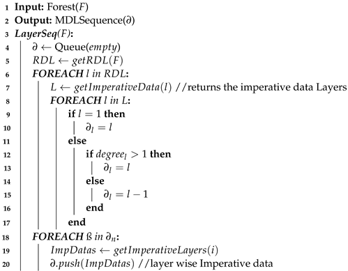 |
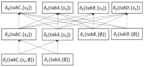
Figure 8.
MDL sampling.
5.2. Sampling Criteria
Sampling with criteria is a statistical method for selecting a sample of data from a larger population using specific conditions or criteria. This method has been frequently employed in previous research to represent the population that satisfies specific requirements or possesses particular characteristics.
We denote sampling criteria with , which indicates that C is the criteria of relation, R, with x tuples in the sampling layer, . We achieve the sample, , of relation, R, in sampling layer, , with the criteria, , using Equations (3) and (4). It indicates that the criteria, , must be satisfied for an element of tuple x to be included in the sample, .
We apply two types of criteria for sampling fresh leaf at the first layer and sample leaf at the layered limbs at the higher layers. These two types of criteria depend on the unary and N-ary filters, respectively.
Unary Filters: The unary filter refers to static or parameterized filters based on the attributes of a relation. In the case of conditions inside a loop, we include a range of criteria in the first layer sampling. We express it with . It indicates that the unary filter, , must be satisfied for an element of a tuple x in a relation, R.
In the criteria of the first sampling layer, we combine all unary filters across all statements in a procedure. We express the criteria of relation in the first sampling layer, , using the following equation:
N-ary Filters: The N-ary filter refers to dependent filters and joining conditions with other relations or declarative expressions. We express it with . It indicates that the N-ary filter, , must be satisfied for an element of a tuple x in a relation, R.
In the criteria of the higher sampling layer, we combine all N-ary filters at a layer, . We express the criteria of relation in the higher sampling layer, , using the following equation:
The existing query parser method determines the filter condition for each table, view, or table variable. It analyzes the syntax of the SQL code and finds the procedure’s statements to create a parse tree, where CFG shows the dependency between statements. This tree structure has a top-level node for the stored procedure and child nodes for its name and parameters. SQL statements in the procedure are the remaining child nodes. Each SQL statement in the stored procedure has its own parse tree, which reflects its structure. The top-level node in this individual statement tree structure depicts the SELECT statement, while child nodes represent the columns to select, the table to select FROM, and the WHERE clause filter condition.
5.3. Sampling Algebra
Sampling algebra refers to a relational algebra for expressing DDL queries to generate imperative samples in relational databases. We utilize the forest data structure to develop sampling algebra. We follow the bottom-up traversing of MDL layers to sequence the DDL expressions. We express the sampling algebra for DDL queries that utilize unary and N-ary filters in Figure 9.
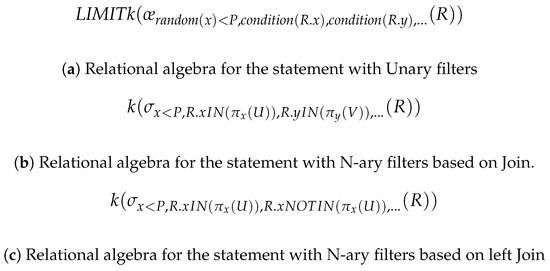
Figure 9.
Sampling algebra for sampling expressions.
In Figure 9a, we express the sampling algebra for the root nodes of the sampling forest, using the unary filters in Equation (5). We observe that the sampling statement contains only one relation, R, and that it defines statement criteria based on the relation’s attributes. It combines a sampling technique with the static or parameterized valued criteria to generate the sampling data from the statement. In Figure 9b,c, we express the sampling algebras for the remaining nodes of the sampling forest, using the N-ary filters in Equation (6), based on JOIN and LEFT JOIN, respectively. We observe that the sampling statement of relation R relates multiple relations, U and V, and that it defines statement criteria based on the join condition using the IN operator. We design the relational algebra such that the attribute of R must exist in those of U and V. In the case of a left join (for example, a left join with U), we design an additional NOT IN.
5.4. Sampling Expression
Sampling expression refers to generating queries for sampling that utilize sampling algebra. We utilize table-level samples rather than view-level samples in each MDL layer. Sampling from the view may yield an inaccurate depiction of the complete data distribution if it originates from a subset of data subject to particular conditions. If the view excludes specific subsets of the data, this becomes especially problematic.
On the other hand, table-level sampling requires physically storing data; it creates overhead. However, it also produces accuracy in sampling from sampled data from the upper layers. Our cost model considers the sampling cost that includes this overhead.
We represent the sampling expression using DDL statements, called sampling statements, that utilize the sampling algebra in Figure 10. We generate samples in a sampling layer for a relation, so each node contains a distinct data source. We name each data source by following a naming convention (naming conventions for a sampling source combine the relation name and sampling layer number, concatenating all the values of the parameter of a procedure). It ensures the use of sample data from a relation for appropriate parameter settings. Figure 10a, Figure 10b, and Figure 10c represent sampling statements from the relational algebra in Figure 9a, Figure 9b, and Figure 9c, respectively.
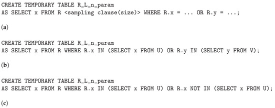
Figure 10.
Sampling expressions. (a) Expression for the statement with unary filters; (b) Expression for the statement with N-ary filters based on JOIN; (c) Expression for the statement with N-ary filters based on LEFT JOIN.
6. Sampling Control Logic Algebraization
Sampling control logic algebraization refers to sampling the control logic with the scale factor, f, using the algebraization technique. We use the sampling algebraization method to sample loops. In the case of branches, we do not sample branches; however, we sample data based on the execution path. The sampling twigs from the forest represent samples from the imperative control region. We employ the algebraization method to sample twigs for data sampling with the scale factor.
We apply algebraization techniques for sampling control logic using scale factor. We transform the loop. If there are multiple nested loops, we follow the same technique. We sample loops through stridden sampling. It selects the iteration by transforming loops into regular skips, which involves skipping a fixed number of elements or iterations between each selected element or iteration. This technique is useful to determine a certain percentage of total loop numbers; for example, if we want to determine the scale factor of 20 percent of the total iterations, we can process every fifth (100/20) element.
This method is faster because it does not check the data but rather deals with only the looping criteria. On the other hand, we are able to use the same scale of sample size in the data sampling when measuring loop counts.
We use the following algebraization method to sample loops:
Figure 11 represents the algebraization technique for loop sampling. Figure 11a shows the original loop statement. Figure 11b represents the relational algebra expression for loop sampling.
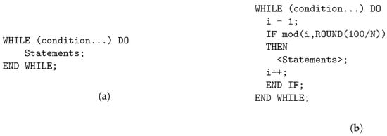
Figure 11.
Relational algebra for loop sampling. (a) Original loop statement; (b) Sampling loop.
7. Agile Approximate Processing
Agile approximate processing refers to an approximate processing method to achieve imperative samples in a best-effort manner within a permissible query time. Suppose the imperative data of a relation evolve through a series of dependent consumer statements, , , ,… . A complete imperative sample utilizes all the consumer statements and produces a sample at the root. Agile approximate processing enables the execution of imperative samples within a permitted query time that utilize a number of intermediate statements (i.e., any statements preceding ). Furthermore, it continues to complete imperative samples. It utilizes the complete imperative sample if it is available, rather than the best-effort imperative sample.
The problem of agile approximate processing is identifying the beneficial imperative samples within a permitted query time and replacing the sample with the original data source. It employs two MDL sampling techniques: (i) cold sampling and (ii) hot sampling. Cold sampling completes the MDL sampling to generate imperative data samples. On the other hand, hot sampling provides imperative samples at any layer based on a permissible time.
We provide an intuition for the agile approximate in Figure 12. Suppose we have a threshold cost at which we are allowed to perform sampling and processing of the procedure. Agile approximate processing estimates the cost of sampling at each layer, starting from the leaf (, , ,…), followed by the procedure processing. It finds the lowest benefit of approximate processing at the threshold cost. The lowest benefit permits sampling from the highest possible layer, which produces more targeted samples. Meanwhile, if it finds a valid cold sampling, it utilizes the cold sampling for approximate processing.

Figure 12.
Agile approximate processing.
7.1. Cold Sampling
Cold sampling refers to the complete MDL sampling of every sampling layer until the root and storing the final layer of sampling for approximate processing. This process is costly; however, it provides more accuracy. Forester performs this method in the background and performs agile approximate processing. If it finds a valid cold sample within the permitted query time, it uses cold samples in approximate processing. This sampling method is also used for precomputed sampling-based approximate processing.
Let there be n sampling layers: , , and . Cold sampling completes the sampling at each layer and provides the imperative sample at layer . We provide the mechanism of cold sampling in Algorithm 3, where it produces the imperative sample at a layer and deletes that of the preceding layer.
| Algorithm 3: Algorithm for Cold Sampling. |
 |
7.2. Hot Sampling
Hot sampling refers to the process of MDL sampling, where it may not complete the sampling of every layer until the root and stores the intermediate or final layer sampling for approximate processing. This sampling method is also used for runtime sampling-based approximate processing.
In this process, MDL sampling performs the sampling of an ascending subset of layers, from leaf to root, based on benefit estimation in runtime. It performs similarly to cold sampling, if it completes the sampling of every layer. In this technique, the latest layer of sampling can be stored temporarily for frequent use or erased after the processing of a procedure.
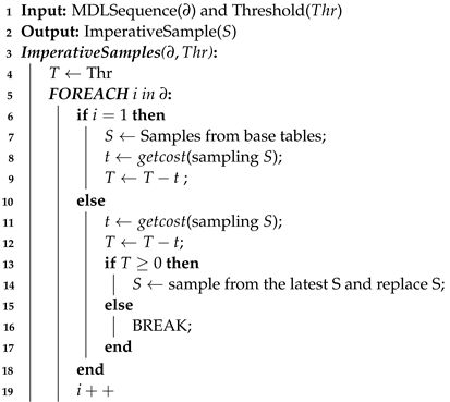
Let there be n sampling layers: , , and . Hot sampling may not complete the sampling at each layer and provide the imperative sample at any layer between and . We provide the mechanism of hot sampling in Algorithm 4, where it produces the imperative sample at a layer based on benefit estimation using a threshold and deletes that of the preceding layer. The threshold value indicates the permitted query time for hot sampling. We continue to estimate the sampling cost to sample at the upper layer until it reaches the threshold time. We estimate the sampling cost of each layer using the forest data structure.
| Algorithm 4: Algorithm for Hot sampling |
 |
7.3. Cost Model for Agile Approximate Processing
Our cost model searches for incremental benefits at the highest possible RDL by comparing the agile approximate processing cost estimate of a procedure () to the threshold cost (T). We express the benefit using the following formula:
We estimate the agile approximate processing cost, , using the following formula:
where is the total sampling cost up to the sampling layer ∂, and is the sampling-aware procedure cost.
Sampling Cost: This refers to the total execution time of sampling statements. In the case of cumulative sampling cost, up to the sampling layer, ∂, it refers to the sampling cost of the imperative samples of all relations up to the layer ∂, as determined by the sampling forest data structure.
where, refers to the sampling cost of each RDL within a relation r (, where R is all the relations in a procedure), as determined by the sampling forest data structure.
Sampling-aware procedure cost: This refers to the total execution time of sampling-aware statements within a procedure after replacing the base data sources with the sampled data sources. We represent the sampling-aware procedure cost as follows:
where s is the statement of a procedure.
The statement cost is represented by the following equation:
where is the total processing time of s, and is the total processing time of all the dependent ancestor statements without s.
Threshold Cost: This refers to the total execution time of the approximate processing of an imperative procedure using base-relation samples. We denote it as T. We estimate the threshold cost based on agile approximate processing using the samples of the first sampling layer, where ∂ = 1. If we apply the existing AQP techniques for the approximate processing of an imperative procedure, it produces the threshold cost. Hence, finding the benefit over the threshold cost shows the better performance of our algorithm.
Assumption
Sampling Forest Data Structure Maintenance: During procedure construction, we construct the sampling forest data structure. We store it as metadata for a procedure. When we invoke the procedure with the FORESTSAMPLE clause for approximate processing, we utilize this information. We clear this information when we drop the procedure.
Historical Data Maintenance: As historical data, we store the sampling cost of each layer and the processing cost of a procedure employing each sampling layer for a given parameter setting and time flag.
MDL Sampling Maintenance: We always materialize the view in each layer in MDL sampling. We store only the final layer sampling in the MDL sampling as historical data for a parameter setting. We delete the sampling generated in intermediate layers. We maintain this storage for MDL sampling until the procedure’s relations are updated. We assume that the OLAP database system deletes the sampling when it updates those relations.
8. FORESTSAMPLE Clause
We propose a clause that utilizes a sample size during the calling procedure. The calling procedure, incorporating the proposed clause, comprises (i) exploiting sampling at runtime; (ii) rewriting the procedure; and (iii) executing the rewritten procedure on the sampled data.
Let the scale factor, f, be 0.2. We call the as follows:
CALL example_procedure(param value,...) FORESTSAMPLE (0.2)
9. Optimization Process
9.1. Optimization Workflow
Optimization Approach: Our optimization strategy is based on the following two principles: (i) generating a more targeted sample by incorporating conditions, multi-level relationships between relations, and imperative logic sampling; and (ii) providing quick runtime approximation results by analyzing the tolerable subset layer sampling from MDL sampling.
We show our total optimization process in Figure 13. We call a procedure using the FORESTSAMPLE clause to perform approximate processing. It first checks for valid cold samples to perform approximate processing. Otherwise, it performs hot sampling. After it decides the sampling method, it starts sampling and rewrites the procedure for approximate processing.
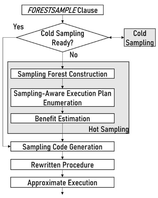
Figure 13.
Optimization process.
9.2. Optimization Steps
Forester optimization has five major steps, as follows: (i) forest representation, where the input is the data and control flow graphs of the imperative procedure and the output is the Forest graph representing the imperative data structure and control logic; (ii) MDL construction, where the input is the forest data structure and the output is the series of sampling layers of all the imperative data; (iii) cold sampling formulation, where the input is the sampling layers and the output is the final layer samples; (iv) hot sampling, where the input is the output of cold sampling and sampling layers and the output is the latest layer sampling from the subset of sampling layers; and (v) sampling control logic, where the input is the procedure script, and the output is the rewritten procedure script.
9.3. Process of Agile Approximate Processing
The agile approximate processing in Forester consists of the following five significant steps: (i) a hot sampling cost estimation, which continuously estimates the cost of cumulative sampling layers; (ii) a procedure cost estimation, which continuously estimates the cost by replacing the relations with the latest sampling layers; (iii) a benefit estimation, which continuously measures the benefit of each progressive sampling compared to the threshold cost; (iv) an approximate processing employment, which applies the steps from (i) to (iii) in runtime after the final benefit estimation in step (iii); and (v) conducting cold sampling in the background for frequent approximate processing when it is complete.
9.4. The Lowest Benefit-Aware Execution Plan
We enumerate all sampling-aware execution plans and select the one with the lowest benefit in step 3 of optimization. The lowest benefit permits the deepest possible layer of sampling, which includes a more targeted sample for the approximate processing of the imperative procedure.
We formulate the lowest benefit-aware execution in Algorithm 5. First, we check the availability of cold sampling. If we obtain valid cold sampling, we use it for hot sampling using ; otherwise, it seeks the plan with the lowest benefit by enumerating all the possible plans using .
| Algorithm 5: Algorithm for Hot sampling Construction in Forester |
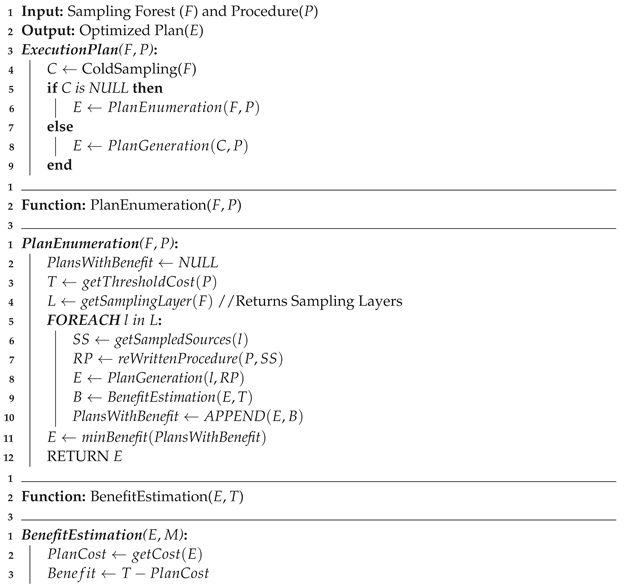 |
We enumerate each plan that includes an MDL layer sample with the necessary rewritten procedure. Thus, a procedure has a maximal number of alternative execution plans that corresponds to the number of MDL layers in the sampling forest.
We measure the benefit of each generated plan relative to the threshold cost using and select the plan with the lowest benefit.
10. Accuracy of Sampling Generation
Forester selects high-quality, targeted samples for the approximate processing of an imperative procedure. Initially, it samples from the base relations at the first sampling layer by combining a sampling technique with all the unary filters, using Equation (5). It ensures that the sample data are applicable at the first level for all types of data distribution. In the subsequent layer, Forester samples from the previous samples of the most recent sampling layer of relations, using the same sampling technique as the previous sampling layer, and N-ary filters with Equation (6). It refines the samples from the previous sampling layer of relations by removing the data from the previous samples that cannot be selected. We represent it using the relational algebra in Figure 14, where Forester removes the tuples at the higher layer from the previous layer. It continues the process till it finds the final sampling layer of a relation.

Figure 14.
Tuples removal at the higher sampling layers in Forester.
Existing AQP techniques can only generate samples at the first level of the first statement containing a relation with criteria. In contrast, Forester improves sampling at the first layer by integrating all the unary filters of a relation across all the statements within a procedure. In addition, it takes into account the interdependencies between multiple statements and generates high-quality, targeted samples for the approximate processing of the imperative procedure.
Accuracy in imperative logic sampling: Forester produces a high-quality sample that takes imperative logic into account. It executes imperative logic using appropriate sample data. It is able to execute imperative logic using data from the first sampling layer or higher. In both cases, there is no possibility that the tuples in Figure 3 will satisfy an imperative condition. It guarantees that no unnecessary iteration, branch, or function call is executed with data that have no possibility of being selected.
11. Semantic Preservation of Procedure
Preserving semantics, as it pertains to approximate queries in a relational database, entails permitting a degree of approximation in the results while preserving the intent or meaning of an imperative procedure. This becomes especially significant when dealing with extensive datasets or when fast responses are critical.
We transform the original query into an equivalent form that is amenable to approximate processing. We replace certain original data sources with their approximate counterparts, which are imperative samples. Imperative data evolve from the dependent statement; however, it includes either the subset or the entire data of a relation. Thus, imperative samples are proven to be approximate counterparts of the original data.
12. Experiment
This section discusses the evaluation of Forester. In Section 12.1, we discuss the overall settings for our experiment, and in Section 12.2 and Section 12.3, we discuss the experimental results.
12.1. Experimental Settings
12.1.1. Workload
The OLAP (online analytical processing) workload, which involves imperative procedures in a data warehouse or data mart, is our sole focus. Our synthetic OLAP workload for imperative procedure approximate processing investigates the following facts: (i) Data distribution: well-behaved data with a predictable distribution work best for approximate analysis. The error limits of AQP techniques may be unreliable if the data are skewed or have outliers. (ii) Procedure kinds: Some OLAP procedures can be approximated better than others. A statement in a procedure that uses aggregation functions over a lot of rows is a good choice for approximate processing. An OLAP procedure has multiple dependent statements with imperative logic (loops and conditionals). (iii) Error tolerance: Application and user needs determine acceptable error levels. Some applications need precise answers, while others can handle a little error. (iv) Statement complexity: Approximate processing works better for simple statements than complex ones. Simple statements have a smaller search area, making approximate solutions with a tiny error bound easier to find.
Approximate processing of imperative procedures provides approximate results for procedures faster than accurate procedure processing. Approximation processing is generally employed in exploratory data analysis, data visualization, and large-scale data processing. We synthesize fifteen imperative procedures (available at: https://github.com/arifkhu/Forester.git, accessed on 31 December 2023) in our workload using the TPC-DS with a database size of 1 GB that covers the following aspects: (i) multiple statements with loops and branches; and (ii) a last statement that contains aggregate functions (i.e., average).
12.1.2. Baseline Evaluation
To the best of our knowledge, we have not found research that deals with the approximate processing of imperative procedures to compare Forester. Currently, we are able to approximate the processing of procedures using the existing AQP techniques.
AQP for the procedure (AQPP): This algorithm is derived from the deployment of an existing approximate query processing technique, utilizing query time sampling for the approximate processing of an imperative procedure [1]. The original work [1] was applied to declarative queries. In the context of imperative procedures, we apply this technique to statements that contain base relations and consume data directly from the database.
AQPP determines that the sampling operator allows queries to be conducted over ad-hoc random samples of tables, that samples are computed uniformly over data items qualified by a columnar basis table, and that the single query approximation uses tuples sampling regarding a table. Figure 15 illustrates an example for our baseline. It shows that AQPP is able to accomplish the task in example 2, where TABLESAMPLE is a sampling operator and scale factor is one. It indicates that it only identifies a one percent sampling from the base tables, , , , and , with criteria within a single statement.
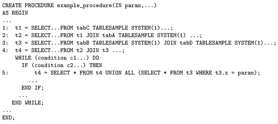
Figure 15.
Example 2: traditional approximate query processing for an imperative procedure.
12.1.3. Physical Environment
We present our experimental findings using the SAP HANA in-memory database, which is publicly accessible at www.sapstore.com, accessed on 1 June 2020. We utilize a Python library, pyhdb, that provides an interface to communicate with the database. Our machine features 45 Silver 4216 2.10GHz Intel Xeon (R) processors and 512GB of RAM. In the case of fewer resources, our algorithm may find a difference in cost estimation. However, it shows the same improvement over the baseline approach.
We use the SAP Hana in-memory database because it supports table variables in imperative procedures like other modern DBMSs, such as SQL Server, etc. As a result, the results produced in SAP Hana also represent the same performance in other DBMSs that support table variables in an imperative procedure. In the case of PostgreSQL, Oracle, etc., we need to use temporary tables instead of table variables.
12.1.4. Performance Measures
We identify the following performance measures to evaluate Forester.
Accuracy: This metric compares the approximation processing system’s results to the exact ones. We utilize a numerical error measure (i.e., relative error (RE)) to quantify the accuracy. We express the formula for the accuracy as follows:
where n is the number of results and and are the exact and approximate results in measuring the average of a projection in the final statement of the ith procedure.
Speed: Speed compares the total processing time of an imperative procedure with approximate processing to the same procedure without approximate processing. The following is a typical formula for measuring speed:
where the total processing time without approximate processing refers to the overall procedure execution time without approximate processing, and the total processing time with approximate processing refers to the overall time to process the procedure, which includes the compilation time, to generate the execution plan, and the execution time, to process the sampling and approximate processing of the procedure.
In query-time exploratory analysis, accuracy and speed are essential metrics for approximate processing. When using exploratory analysis, users usually anticipate correct and significant insights from the results. Ensuring accuracy guarantees that the outcomes displayed to users accurately reflect the distribution of the underlying data. Even though accuracy is crucial, there are situations where a small loss of accuracy is acceptable in return for appreciable increases in speed. To get the best results in approximate processing, the trade-off between speed and accuracy is frequently taken into account. Although speed and accuracy are important metrics, it’s also important to take other factors, like scalability, robustness, sensitivity, etc., into account. We discuss these factors in the experimental section.
12.2. Experimental Results for Overall Evaluation
This section evaluates the overall performance of Forester. In Section 12.2.1 and Section 12.2.2, we evaluate the accuracy and speed of Forester, respectively. In Section 12.2.3, we evaluate the performance of precomputed sampling using the available cold sampling. In Section 12.2.4, we evaluate the targeted sampling generation in MDL sampling. Next, we show the compilation overhead in Section 12.2.6. We discuss optimal performance in Section 12.2.5.
12.2.1. Evaluation of Accuracy
Figure 16 shows the overall performance evaluation using our workload, where Figure 16a depicts the accuracy of the sample across all of our procedures. We use a 1GB database and a parameter setting of 2000–2020 to conduct this experiment. In this experiment, we use the scale factor . We also conduct sensitivity testing by varying the database size in Section 12.3.3, varying the parameters in Section 12.3.4, and varying the projection columns in Section 12.3.2. For example, we call the P1 procedure as follows:
CALL P1(2000, 2020) FORESTSAMPLE (0.2);
Forester performs with more than 95% accuracy in all the cases using agile processing, whereas AQPP shows below 95% in the majority of cases. We report all the data for overall accuracy in Appendix A.1. In each case, Forester finds the MDL sampling at the second sampling layer. We discussed in Section 10 that the higher levels of MDL layers produce more targeted data, and we will evaluate the MDL sampling in Section 12.2.4. For example, procedure uses a sample from the second sampling layer, which generates a more targeted sample than the first layer. AQPP is able to use only the first sampling layer. Hence, Forester obtains higher accuracy than AQPP.
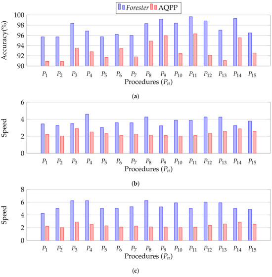
Figure 16.
Overall performance evaluation. (a) Performance evaluation for accuracy; (b) Performance evaluation for speed-up; (c) Performance evaluation for speed-up using only cold sampling.
Figure 16.
Overall performance evaluation. (a) Performance evaluation for accuracy; (b) Performance evaluation for speed-up; (c) Performance evaluation for speed-up using only cold sampling.

12.2.2. Evaluation of Speed-Up
Figure 16b illustrates the approximate processing performance of all procedures during the runtime. We utilize the same setting as in Section 12.2.1 to conduct this experiment.
Forester is faster by more than four times in the majority of cases, whereas AQPP is slower in the majority of cases. We report all the data for overall speed in Appendix A, Table A2. We discussed in Section 10 that the higher imperative samples at higher levels produce fewer rows. We discuss the number of rows in MDL sampling in Section 12.2.4. Processing with fewer rows is faster. On the other hand, generating imperative samples in higher layers requires additional processing costs. In this case, our cost model finds the benefit of producing the samples.
Overall, Forester obtains a higher speed. For example, procedure uses a sample from the second sampling layer, which generates fewer rows in imperative samples than the first layer. AQPP is able to use only the first sampling layer, which contains a larger number of rows of samples. Hence, Forester obtains a higher speed than AQPP.
12.2.3. Evaluation of Precomputed Cold Sampling
We conducted the experiments to observe the speed of Forester if the cold sample is precomputed and valid. As we discussed, some DBMSs store precomputed sampling for future approximate processing. In order to show the performance of approximate processing with precomputed sampling, we assume that the cold sampling was stored in DBMSs previously, and we perform approximate processing using cold samples. In this case, we do not utilize agile processing using hot samples. Hence, the processing cost of sampling generation is not taken into account.
Figure 16c illustrates the approximate processing performance of all procedures that utilize cold sampling. We utilize the same setting as in Section 12.2.1 to conduct this experiment.
We observe that cold sampling is faster. We report all the data for precomputed approximate processing in Appendix A, Table A2. In the case of hot sampling, Forester uses best-effort sampling to determine the optimal plan, which requires additional cost to find samples. In the case of cold sampling, we already have the samples, which are stored. Moreover, cold sampling contains the least number of rows, as discussed in Section 12.2.4, and takes less time for approximate processing. However, if the state of the database changes, cold samples are not valid. As a result, the lifespan of a cold sample is very short. Hence, hot samples are more reliable than cold samples.
12.2.4. Evaluation of MDL Sampling
We conducted this experiment to evaluate how MDL sampling produces more targeted samples. We demonstrate the decomposition of MDL sampling using . Figure 17 depicts the sample size for each relation from the leaf to the root layers. We observe that the sample size of a relation decreases as the sampling depth increases, while the overall accuracy remains unchanged. This occurs because Forester generates the sample for the deeper layer by contemplating dependencies with other relationships in the same layer, using samples from higher layers. It reduces the number of rows without affecting the overall approximation; hence, the accuracy remains constant. This experiment demonstrates that Forester produces more targeted samples for all MDL relations.
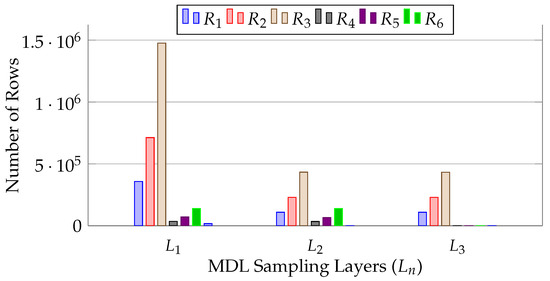
Figure 17.
MDL sampling evaluation.
12.2.5. Evaluation of Optimality
Forester always generates an optimal execution plan using cold sampling because it takes the sample from the root. However, it may sacrifice some optimality in hot sampling in the case of smaller relations and computations, as discussed in Section 12.1.1 and Section 12.2.4. Forester will be very useful in generating an optimal plan using cold sampling because, in a real scenario, OLAP procedures deal with a large amount of data, and the frequent synchronization of the OLAP database from OLTP transactions is costly, except for the HTAP environment. In the case of the HTAP environment, Forester frequently performs hot sampling because cold sampling may be valid for a shorter period of time as HTAP deals with real-time data for OLAP query processing.
12.2.6. Evaluation of Compilation Overhead
Figure 18 depicts the Forester compilation overhead. We observe that it creates a negligible amount of compilation overhead, in all cases less than 0.5 s. Consequently, it is highly beneficial in any DBMS.

Figure 18.
Compilation overhead of Forester.
12.3. Experimental Results For Sensitivity
We evaluate the sensitivity performance of Forester. In Section 12.3.1, we vary sample sizes to evaluate the sensitivity of sample size. We evaluate the sensitivity of projection by varying the projection in Section 12.3.2. In Section 12.3.3, we evaluate scalability by expanding the database size. In Section 12.3.4, we undertake parameter sensitivity testing by changing the parameters of the procedure. We use a subset of our workload with distinct categories that represent the sensitivity performance of all workload procedures. We selected two procedures, and , containing a loop and a branch, respectively.
12.3.1. Evaluation of Sample Size Sensitivity
We conducted this experiment to observe the robustness of Forester in the case of sample size variation. We keep the settings that were set out in Section 12.2.1, except for the sample size. We vary the sample sizes using 0.2, 0.3, and 0.4 to observe the accuracy and speed.
Figure 19 shows that in both cases of P1 and P2, Forester achieves more than 95% accuracy and more than three times faster speed, which definitely outperforms AQPP. We report the complete data in Appendix B.
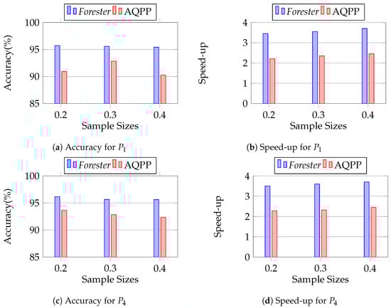
Figure 19.
Evaluating the sample size sensitivity of Forester.
We have an interesting observation in accuracy measuring in both Forester and AQPP. Forester always guarantees similar accuracy for all sample size variations because it samples in a targeted manner at the initial layers, using leaf sampling based on sample size. It continues sampling the upper layers by reducing data that are not responsible for the imperative sample. Thus, the samples become more targeted, making the approximate processing faster. On the other hand, AQPP cannot guarantee a similar accuracy for sample size variation because it only samples from the relations based on sample size.
12.3.2. Evaluation of Projection Sensitivity
We conducted this experiment to observe the robustness of Forester in the case of projection column variation, because exploratory data analysis may require multiple columns. We vary the projection column in the final statement in the procedure and keep the other settings set out in Section 12.2.1. We use , , and projection columns for P1 and , , and for , to observe the accuracy and speed.
Figure 20 shows the performance of Forester in variation of projection columns. We observe that, in all cases of accuracy and speed, Forester outperforms AQPP. We report the complete data in Appendix C. The reason is the same as in Section 12.2.1 and Section 12.2.2.
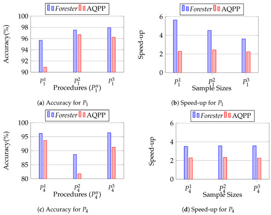
Figure 20.
Evaluating the projection sensitivity of Forester.
12.3.3. Evaluation of Scalability
We conducted this experiment to observe the scalability of Forester in the case of larger database sizes. We vary the size of the database, using 50 GB and 100 GB, while keeping the other settings set out in Section 12.2.1. We observe that Forester achieves more than 95% accuracy in all the cases of P1 and P2.
Figure 21 shows the performance of Forester in variation of database sizes. Here, we observe that Forester finds the benefit of the root layer in MDL sampling in the cases of 50 GB and 100 GB, whereas we find the benefit at the second layer in 1 GB size. Thus, we can say that Forester produces the optimal plan in the case of large data.
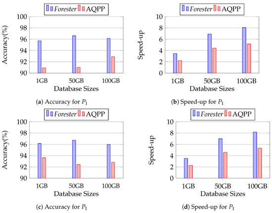
Figure 21.
Evaluating the scalability of Forester.
12.3.4. Evaluation of Parameter Sensitivity
We conducted this experiment to observe the scalability of Forester in the case of computational variation. We vary the parameter to make it larger in loop processing while keeping the other settings set out in Section 12.2.1. We utilize three variants of P1, where we determine the loop iterations at 20, 40, and 60, respectively.
Figure 22 shows the performance of Forester in variation of parameters. We observe that Forester achieves more than 95% accuracy in all the cases of P1, which outperforms AQPP. Here, we observe that Forester finds the benefit at layer 2 in MDL sampling in the case of 40 and 60 iterations. On the other hand, Forester also capable of imperative logic sampling based on sample size. For example, it iterates 13, 25, and 38 times in the case of a sample size of 0.2. As a result, we achieve more improvement in speed for larger iterations.
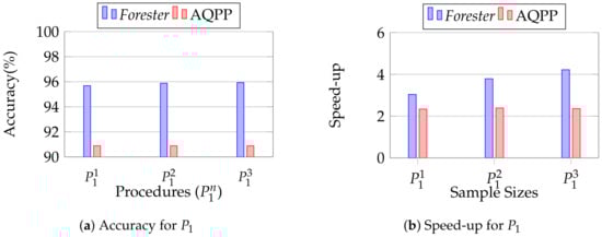
Figure 22.
Evaluating the parameter sensitivity of Forester.
13. Related Works
Previous studies in sampling-based query-time exploratory data analysis, discussed in Section 13.1, utilized only declarative queries. They were unable to solve the issues that utilized imperative procedures containing imperative data and control logic. On the other hand, previous studies on the approximate processing of a procedure, discussed in Section 13.2, limited themselves to ad-hoc random sampling table-based approaches that are able to sample only base relations. They are unable to sample imperative data and control logic. Apart from this, previous studies on the control region sampling-based approach, discussed in Section 13.2, only dealt with sampling loops or branches inside a procedure. They, however, cannot deal with the imperative data inside a procedure.
To the best of our knowledge, we are the first to explore sampling-based query-time exploratory data analysis that utilizes imperative structures such as imperative data and control regions in procedures. We found no research work in this area, which represents the originality of our work. We limit ourselves to studying the related work in those areas, such as exploratory data analysis for approximate query processing and sampling for approximate processing, which are related to individual parts of our research. Hence, we found fewer works that are relevant to our work.
13.1. Literature on Exploratory Data Analysis for Approximate Query Processing
Explored data analysis (EDA) is significant because data scientists require tools for fast data visualization and want to discover subsets of data that need additional drilling-down before performing computationally expensive analytical procedures. Meng [1] covers query-time sampling with stratified and hash-based equi-join samplers to facilitate approximate query processing for exploratory data research. However, they only sample from base tables in a query, not dependent queries’ data sources.
The use of exploratory data analysis in approximate query processing has also drawn attention from researchers. Fisher [6,7] discussed the usage of queries that function on progressively larger samples from a database, to allow people to interact with incremental visualization, and that handle incremental, approximative database queries, trading speed for accuracy by taking a sample from the entire database, enabling the system to answer questions quickly. In order to reduce the requirement for repeated exploratory searches, Kadlag [8] recommended using exploratory “trial-and-error” queries.
Numerous studies on EDA have been carried out; for example, Javadiha [9] identifies the shortcomings of conventional table-based techniques for sensor technology analysis, while Yang [10] addresses exploratory graph queries.
In relational databases, exploratory data analysis (EDA) is an essential tool for deciphering the underlying relationships, patterns, and trends in the data [11,12,13,14,15,16,17,18,19,20]. There are numerous research articles and resources that cover different facets of EDA in the context of data stored in relational databases, even though there may not be a single study that is exclusively focused on EDA in relational databases. For instance, Savva [21] explains how predicting the outcomes of aggregate queries is one way that machine learning can be utilized to speed up the data exploration process. Nargesian [22] is a recent data-driven framework that restructures queries to assist users in locating relevant data entities in situations involving large dimensionality and a lack of in-depth data understanding.
13.2. Literature on Sampling for Approximate Processing
Our approach adapts the existing sampling method by sampling from top leaf, which is the relation of sampling from base. One efficient technique to handle a large number of requests on a large database is to use approximate query processing using relatively small random samples. Multidimensional cluster sampling [23], stratified random sampling of the original data [24,25,26,27], sampling databases that follow the same distribution for specific fields [28], adaptive random sampling [29], and simple random sampling [30] algorithms are proposed for approximate query processing. However, in the case of multi-dependent statements, it is not possible to sample from all the statements with imperative structures inside a procedure.
Two-stage sampling [2,3] and adaptive sampling [4] have been studied in large and heterogeneous populations. Two-stage cluster and adaptive sampling is a simpler version of multi-stage sampling that can work when deeper multi-stage sampling is not necessary. It is useful when the population is naturally clustered and sampling individuals from the total population is not necessary.
In multi-layer sampling for approximate imperative procedure processing, two-stage cluster and adaptive sampling techniques have the following drawbacks: (i) Biased sample: the problem with this method is that, in the first stage of a two-stage sampling technique, it is possible to select a biased sample. This can occur if the first-stage sampling frame does not accurately represent the population. (ii) Data synchronization: coordinating the data flow and ensuring the sampled data match the procedure steps may need careful planning and monitoring (i.e., an imperative method may use loops or conditionals). (iii) Dependent layer criteria: two-stage sampling of sample data in multistages for the same data source. In a procedure, layer sampling of a relation may depend on layer sampling of other relations, due to joining. Thus, two-stage sampling struggles to determine sample criteria. Finally, (iv) parameter setting: two-stage sampling might generate bias or inconsistencies if the sampling method or parameters change between stages.
Zar [5] introduced probabilistic samplers in the random-bit model, which is aware of loops and conditioning. However, in the case of the multi-statement imperative procedure, we are focusing on generating samples through dependent statements. In order to acquire that, we sample loops that are well representative of the dependent data distribution. On the other hand, we do not sample branches because they lose some representative samples. As a result, systematic loop sampling fits well for sampling imperative data rather than probabilistic sampling.
14. Future Scope
We acknowledge the threats and limitations of our research. Our cost estimation for agile approximate processing depends on some estimated values, such as sampling layer costs, procedure costs, and threshold costs. If the values are not properly maintained or estimated, our algorithm may have difficulties finding benefits for agile processing. In this research, we utilize historical data for the cost estimation of sampling layers, procedure costs, and threshold costs to find the benefit of agile approximate processing. In our future work, we will extend our work to find some efficient techniques for estimating those costs.
15. Conclusions
Database administration and computing efficiency have advanced significantly with query-time approximate processing for imperative algorithms. Through the use of novel approaches that integrate the concepts of query optimization and data approximation, Forester has the potential to completely transform the ways in which data are stored, accessed, and examined in intricate database systems.
Agile approximation processing represents a major paradigm shift in our understanding of the trade-off between processing speed and result accuracy, as well as a significant change in the design and execution of stored procedures. Through the precise adjustment of the degree of approximation and the incorporation of sophisticated error handling procedures, this new methodology enables database administrators and developers to traverse the complex terrain of data administration with unparalleled accuracy and computing efficiency.
Additionally, the fact that this innovative idea was successfully implemented, utilizing forest representation, highlights how approximation approaches may significantly improve the responsiveness and scalability of modern database systems. This innovative approach paves the way for a new era of data-driven insights and empowers organizations to extract actionable intelligence from massive repositories of complex, dynamic data, as the demand for real-time data analytics and streamlined decision-making processes grows.
As we look to the future, the key to achieving previously unattainable efficiency in data management and helping businesses stay ahead in a more competitive and data-centric world lies in the ongoing research and refining of Forester in the approximate processing of essential tasks. The integration of approximation processing is poised to redefine the limits of what is possible in the field of database management and computation as research and development in this area advance, resulting in a new wave of innovation and revolutionary possibilities for the future.
Author Contributions
Conceptualization, M.A.R. and Y.-K.L.; methodology, M.A.R.; formal analysis, M.A.R. and Y.-K.L.; investigation, M.A.R. and Y.-K.L.; data curation, M.A.R.; writing—original draft preparation, M.A.R.; writing—review and editing, Y.-K.L.; visualization, M.A.R.; supervision, Y.-K.L.; project administration, Y.-K.L. All authors have read and agreed to the published version of the manuscript.
Funding
This work was supported by Institute of Information & Communications Technology Planning & Evaluation (IITP) grant, funded by the Korean government (MSIT) (No. 2021-0-00859, Development of a distributed graph DBMS for intelligent processing of big graphs.
Data Availability Statement
We provide a workload with imperative procedures at https://github.com/arifkhu/Forester.git, accessed on 31 December 2023.
Conflicts of Interest
The authors declare no conflicts of interest.
Appendix A. Data for Overall Evaluation
Appendix A.1. Overall Accuracy Measurement Data

Table A1.
Overall accuracy measurement data.
Table A1.
Overall accuracy measurement data.
| Original | Forester | AQPP | |||
|---|---|---|---|---|---|
| Procedure | Results | Results | Accuracy% | Results | Accuracy% |
| 38.66 | 37 | 95.70 | 35.15 | 90.9208 | |
| 38.66 | 37 | 95.70 | 35.15 | 90.9208 | |
| 51.865 | 51.02 | 98.37 | 55.23 | 93.51 | |
| 51.865 | 50.23 | 96.84 | 55.6 | 92.79 | |
| 50.382 | 48.23 | 95.72 | 46.2 | 91.69 | |
| 3658.89 | 3520.23 | 96.21 | 3420.02 | 93.47 | |
| 3255.94 | 3125.23 | 95.98 | 35.23.02 | 91.79 | |
| 58,256.23 | 59,238.2 | 98.31 | 61,235.05 | 94.88 | |
| 57,671.76 | 58,147.01 | 99.17 | 60,025.89 | 95.92 | |
| 254.32 | 250.235 | 98.39 | 235.2 | 92.48 | |
| 1847.38 | 1841.002 | 99.65 | 1779.225 | 96.31 | |
| 3259.23 | 3221.23 | 98.83 | 3002.006 | 92.10 | |
| 269.23 | 261.223 | 97.02 | 245.203 | 91.07 | |
| 5236.001 | 5200.02 | 99.48 | 5002.002 | 95.53 | |
| 51.2 | 53.002 | 96.48 | 55.02 | 90.53 | |
Appendix A.2. Overall Speed Measurement Data
Table A2.
Overall speed measurement data.
Table A2.
Overall speed measurement data.
| Original | Forester | AQPP | |||||
|---|---|---|---|---|---|---|---|
| Procedure | Processing Time(s) | Agile Processing Time(s) | Speed(X) | Processing Time with Pre-Computed Sampling(s) | Speed(X) | Processing Time(s) | Speed(X) |
| 104.2 | 30.20 | 3.45 | 24.63 | 4.23 | 47.15 | 2.21 | |
| 104.6 | 32.09 | 3.26 | 20.84 | 5.02 | 51.79 | 2.02 | |
| 23.43 | 6.73 | 3.48 | 3.76 | 6.23 | 8.10 | 2.89 | |
| 23.18 | 5.05 | 4.59 | 3.72 | 6.23 | 9.27 | 2.5 | |
| 53.47 | 17.70 | 3.02 | 10.65 | 5.02 | 23.25 | 2.3 | |
| 61.15 | 17.03 | 3.59 | 12.15 | 5.03 | 29.12 | 2.1 | |
| 61.49 | 17.17 | 3.58 | 11.64 | 5.28 | 27.33 | 2.25 | |
| 65.23 | 15.31 | 4.26 | 10.43 | 6.25 | 30.77 | 2.12 | |
| 21.01 | 6.50 | 3.23 | 3.99 | 5.26 | 10.04 | 2.09 | |
| 38.67 | 9.41 | 3.89 | 6.56 | 5.89 | 6.56 | 2.02 | |
| 59.38 | 15.34 | 3.87 | 11.85 | 5.01 | 28.55 | 2.08 | |
| 61.47 | 14.43 | 4.26 | 10.22 | 6.01 | 26.04 | 2.36 | |
| 37.89 | 8.91 | 4.25 | 6.42 | 5.9 | 14.68 | 2.58 | |
| 20.03 | 6.16 | 3.25 | 3.99 | 5.01 | 6.97 | 2.87 | |
| 23.15 | 6.12 | 3.78 | 4.74 | 4.88 | 9.08 | 2.55 | |
Appendix B. Data for Evaluating Sample Size Sensitivity
Appendix B.1. Accuracy Measurement Data for Evaluating Sample Size Sensitivity
Table A3.
Accuracy measurement data for evaluating sample size sensitivity.
Table A3.
Accuracy measurement data for evaluating sample size sensitivity.
| Original | Scale Factor | Forester | AQPP | |||
|---|---|---|---|---|---|---|
| Procedure | Results | f | Results | Accuracy% | Results | Accuracy% |
| 38.66 | 0.2 | 37 | 95.70 | 35.15 | 90.92 | |
| 38.66 | 0.3 | 36.95 | 95.57 | 35.89 | 92.83 | |
| 38.66 | 0.4 | 36.89 | 95.42 | 34.89 | 90.24 | |
| 51.23 | 0.2 | 49.26 | 96.15 | 47.97 | 93.63 | |
| 51.23 | 0.3 | 49.01 | 95.64 | 47.56 | 92.83 | |
| 51.23 | 0.4 | 48.99 | 95.62 | 47.32 | 92.36 | |
Appendix B.2. Accuracy Measurement Data for Evaluating Sample Size Sensitivity
Table A4.
Speed measurement data for evaluating sample size sensitivity.
Table A4.
Speed measurement data for evaluating sample size sensitivity.
| Original | Scale Factor | Forester | AQPP | |||
|---|---|---|---|---|---|---|
| Procedure | Processing Time (s) | f | Processing Time (s) | Speed (X) | Processing Time (s) | Speed (X) |
| 104.20 | 0.2 | 30.20 | 3.45 | 47.15 | 2.21 | |
| 104.20 | 0.3 | 29.35 | 3.55 | 44.34 | 2.35 | |
| 104.20 | 0.4 | 28.16 | 3.70 | 42.53 | 2.45 | |
| 10.52 | 0.2 | 3.008 | 3.49 | 4.62 | 2.28 | |
| 10.52 | 0.3 | 2.924 | 3.60 | 4.53 | 2.32 | |
| 10.52 | 0.4 | 2.845 | 3.70 | 4.29 | 2.45 | |
Appendix C. Data for Evaluating Projection Sensitivity
Appendix C.1. Accuracy Measurement Data for Evaluating Projection Sensitivity
Table A5.
Accuracy measurement data for evaluating projection sensitivity.
Table A5.
Accuracy measurement data for evaluating projection sensitivity.
| Original | Projection | Forester | AQPP | |||
|---|---|---|---|---|---|---|
| Procedure | Results | Columns | Results | Accuracy% | Results | Accuracy% |
| 38.67 | 37 | 95.70 | 35.15 | 90.92 | ||
| 50.94 | 49.67 | 97.50 | 49.25 | 96.68 | ||
| 60.52 | 59.27 | 97.91 | 58.23 | 96.26 | ||
| 51.23 | 49.26 | 96.15 | 47.97 | 93.63 | ||
| 24.06 | 26.79 | 88.68 | 28.44 | 81.80 | ||
| 1.12 | 1.08 | 96.42 | 1.01 | 90.17 | ||
Appendix C.2. Accuracy Measurement Data for Evaluating Projection Sensitivity
Table A6.
Speed measurement data for evaluating projection sensitivity.
Table A6.
Speed measurement data for evaluating projection sensitivity.
| Original | Projection | Forester | AQPP | |||
|---|---|---|---|---|---|---|
| Procedure | Processing Time (s) | Columns | Processing Time (s) | Speed (X) | Processing Time (s) | Speed (X) |
| 125.32 | 22.27 | 5.62 | 54.85 | 2.28 | ||
| 103.46 | 22.93 | 4.51 | 42.50 | 2.43 | ||
| 111.23 | 30.89 | 3.60 | 49.77 | 2.23 | ||
| 10.52 | 3.008 | 3.49 | 4.62 | 2.28 | ||
| 10.68 | 3.005 | 3.55 | 4.58 | 2.32 | ||
| 10.68 | 2.995 | 3.56 | 4.75 | 2.24 | ||
Appendix D. Data for Evaluating Scalability
Appendix D.1. Accuracy Measurement Data for Evaluating Scalability
Table A7.
Accuracy measurement data for evaluating scalability sensitivity.
Table A7.
Accuracy measurement data for evaluating scalability sensitivity.
| Original | Database | Forester | AQPP | |||
|---|---|---|---|---|---|---|
| Procedure | Results | Size | Results | Accuracy% | Results | Accuracy% |
| 38.67 | 1 GB | 37 | 95.70 | 35.15 | 90.92 | |
| 39.56 | 50 GB | 38.22 | 96.61 | 36.01 | 91.00 | |
| 41.12 | 100 GB | 39.52 | 96.10 | 39.52 | 92.90 | |
| 51.23 | 1 GB | 49.26 | 96.15 | 47.97 | 93.63 | |
| 53.02 | 50 GB | 51.28 | 96.71 | 49.01 | 92.41 | |
| 55.23 | 100 GB | 53.00 | 95.97 | 51.25 | 92.80 | |
Appendix D.2. Accuracy Measurement Data for Evaluating Scalability
Table A8.
Speed measurement data for evaluating scalability.
Table A8.
Speed measurement data for evaluating scalability.
| Original | Database | Forester | AQPP | |||
|---|---|---|---|---|---|---|
| Procedure | Processing Time (s) | Size | Processing Time (s) | Speed (X) | Processing Time (s) | Speed (X) |
| 104.20 | 1 GB | 30.20 | 3.45 | 47.15 | 2.21 | |
| 3123.21 | 50 GB | 453.07 | 6.90 | 707.28 | 4.42 | |
| 7294.50 | 100 GB | 906.14 | 8.05 | 1414.57 | 5.15 | |
| 10.52 | 1 GB | 3.008 | 3.49 | 4.62 | 2.28 | |
| 315.80 | 50 GB | 45.12 | 6.99 | 69.31 | 4.55 | |
| 736.88 | 100 GB | 90.24 | 8.16 | 138.63 | 5.31 | |
Appendix E. Data for Evaluating Parameter Sensitivity
Appendix E.1. Accuracy Measurement Data for Evaluating Parameter Sensitivity
Table A9.
Accuracy measurement data for evaluating parameter sensitivity.
Table A9.
Accuracy measurement data for evaluating parameter sensitivity.
| Original | Forester | AQPP | ||||
|---|---|---|---|---|---|---|
| Procedure | Results | Parameter | Results | Accuracy% | Results | Accuracy% |
| 38.66 | 2000–2020 | 37 | 95.70 | 35.15 | 90.92 | |
| 38.66 | 2000–2040 | 37.07 | 95.88 | 35.14 | 90.89 | |
| 38.66 | 2000–2060 | 37.09 | 95.93 | 35.14 | 90.89 | |
| 51.23 | 2000–2020 | 49.26 | 96.15 | 47.97 | 93.63 | |
| 51.23 | 2000–2040 | 49.2 | 96.03 | 47.95 | 93.59 | |
| 51.23 | 2000–2060 | 48.15 | 95.93 | 47.9 | 93.49 | |
Appendix E.2. Accuracy Measurement Data for Evaluating Parameter Sensitivity
Table A10.
Speed measurement data for evaluating parameter sensitivity.
Table A10.
Speed measurement data for evaluating parameter sensitivity.
| Original | Forester | AQPP | ||||
|---|---|---|---|---|---|---|
| Procedure | Processing Time (s) | Parameter | Processing Time (s) | Speed (X) | Processing Time (s) | Speed (X) |
| 104.20 | 2000–2020 | 30.20 | 3.45 | 47.15 | 2.21 | |
| 104.20 | 2000–2040 | 29.35 | 3.55 | 44.34 | 2.35 | |
| 104.20 | 2000–2060 | 28.16 | 3.70 | 42.53 | 2.45 | |
| 10.52 | 2000–2020 | 3.008 | 3.49 | 4.62 | 2.28 | |
| 10.52 | 2000–2040 | 2.924 | 3.60 | 4.53 | 2.32 | |
| 10.52 | 2000–2060 | 2.845 | 3.70 | 4.29 | 2.45 | |
References
- Meng, X.; Aluç, G. Exploratory Data Analysis in SAP IQ Using Query-Time Sampling. In Proceedings of the 2021 IEEE 37th International Conference on Data Engineering (ICDE), Chania, Greece, 19–22 April 2021; pp. 2381–2386. [Google Scholar]
- Du, Q.Q.; Gao, G.; Jin, Z.D.; Li, W.; Chen, X.Y. Application of monte carlo simulation in reliability and validity evaluation of two-stage cluster sampling on multinomial sensitive question. In Proceedings of the Information Computing and Applications: Third International Conference (ICICA 2012), Chengde, China, 14–16 September 2012; Proceedings 3. Springer: Berlin/Heidelberg, Germany, 2012; pp. 261–268. [Google Scholar]
- Naddeo, S.; Pisani, C. Two-stage adaptive cluster sampling. Stat. Methods Appl. 2005, 14, 3–10. [Google Scholar] [CrossRef]
- Muttlak, H.A.; Khan, A. Adjusted two-stage adaptive cluster sampling. Environ. Ecol. Stat. 2002, 9, 111–120. [Google Scholar] [CrossRef]
- Bagnall, A.; Stewart, G.; Banerjee, A. Formally Verified Samplers from Probabilistic Programs with Loops and Conditioning. Proc. ACM Program. Lang. 2023, 7, 1–24. [Google Scholar] [CrossRef]
- Fisher, D.; Drucker, S.M.; König, A.C. Exploratory visualization involving incremental, approximate database queries and uncertainty. IEEE Comput. Graph. Appl. 2012, 32, 55–62. [Google Scholar] [CrossRef] [PubMed]
- Fisher, D. Incremental, approximate database queries and uncertainty for exploratory visualization. In Proceedings of the 2011 IEEE Symposium on Large Data Analysis and Visualization, Providence, RI, USA, 23–24 October 2011; pp. 73–80. [Google Scholar]
- Kadlag, A.; Wanjari, A.V.; Freire, J.; Haritsa, J.R. Supporting exploratory queries in databases. In Proceedings of the Database Systems for Advanced Applications: 9th International Conference (DASFAA 2004), Jeju Island, Republic of Korea, 17–19 March 2003; Proceedings, 9. Springer: Berlin/Heidelberg, Germany, 2004; pp. 594–605. [Google Scholar]
- Javadiha, M.; Andujar, C.; Lacasa, E. A Query Language for Exploratory Analysis of Video-Based Tracking Data in Padel Matches. Sensors 2022, 23, 441. [Google Scholar] [CrossRef] [PubMed]
- Yang, C.; Qiao, S.; Özsoyoğlu, Z.M. An exploratory graph query interface for biomedical data. In Proceedings of the 6th ACM Conference on Bioinformatics, Computational Biology and Health Informatics, Atlanta, Georgia, 9–12 September 2015; pp. 527–528. [Google Scholar]
- Nuñez von Voigt, S.; Pauli, M.; Reichert, J.; Tschorsch, F. Every Query Counts: Analyzing the Privacy Loss of Exploratory Data Analyses. In Proceedings of the Data Privacy Management, Cryptocurrencies and Blockchain Technology: ESORICS 2020 International Workshops, DPM 2020 and CBT 2020, Guildford, UK, 17–18 September 2020; Revised Selected Papers 15. Springer: Berlin/Heidelberg, Germany, 2020; pp. 258–266. [Google Scholar]
- Giannakopoulou, S. Query-Driven Data Cleaning for Exploratory Queries. In Proceedings of the CIDR, Asilomar, CA, USA, 13–16 January 2019. [Google Scholar]
- Abeysinghe, R.; Cui, L. Query-constraint-based mining of association rules for exploratory analysis of clinical datasets in the national sleep research resource. BMC Med. Inform. Decis. Mak. 2018, 18, 89–100. [Google Scholar] [CrossRef] [PubMed]
- Ma, C.; Zhang, B. A new query recommendation method supporting exploratory search based on search goal shift graphs. IEEE Trans. Knowl. Data Eng. 2018, 30, 2024–2036. [Google Scholar] [CrossRef]
- Khan, H.A.; Sharaf, M.A. Model-based diversification for sequential exploratory queries. Data Sci. Eng. 2017, 2, 151–168. [Google Scholar] [CrossRef]
- Guo, C.; Wu, Z.; He, Z.; Wang, X.S. An adaptive data partitioning scheme for accelerating exploratory spark SQL queries. In Proceedings of the Database Systems for Advanced Applications: 22nd International Conference (DASFAA 2017), Suzhou, China, 27–30 March 2017; Proceedings, Part I 22. Springer: Berlin/Heidelberg, Germany, 2017; pp. 114–128. [Google Scholar]
- Moritz, D.; Fisher, D. What users don’t expect about exploratory data analysis on approximate query processing systems. In Proceedings of the 2nd Workshop on Human-In-the-Loop Data Analytics, Chicago, IL, USA, 14–19 May 2017; pp. 1–4. [Google Scholar]
- Qarabaqi, B.; Riedewald, M. Merlin: Exploratory analysis with imprecise queries. IEEE Trans. Knowl. Data Eng. 2015, 28, 342–355. [Google Scholar] [CrossRef]
- Gkorgkas, O. Database Content Exploration and Exploratory Analysis of User Queries. Ph.D. Thesis, Norwegian University of Science and Technology, Torgarden, Norway, 12 October 2015. Available online: http://hdl.handle.net/11250/2354160 (accessed on 1 February 2024).
- De Vocht, L. Iterative query refinement for exploratory search in distributed heterogeneous linked data. In Proceedings of the ISWC-DC 2015 The ISWC 2015 Doctoral Consortium, Bethlehem, PA, USA, 12 October 2015; p. 1. [Google Scholar]
- Savva, F. Query-Driven Learning for Automating Exploratory Analytics in Large-Scale Data Management Systems. Ph.D. Thesis, University of Glasgow, Glasgow, UK, 12 January 2021. Available online: https://theses.gla.ac.uk/id/eprint/81907 (accessed on 1 February 2024).
- Nargesian, F. Data-driven recommendations for exploratory query formulation. In Proceedings of the 2014 SIGMOD PhD Symposium, Snowbird, UT, USA, 22–27 June 2014; pp. 31–35. [Google Scholar]
- Inoue, T.; Krishna, A.; Gopalan, R.P. Multidimensional cluster sampling view on large databases for approximate query processing. In Proceedings of the 2015 IEEE 19th International Enterprise Distributed Object Computing Conference, Adelaide, SA, Australia, 21–25 September 2015; pp. 104–111. [Google Scholar]
- Chaudhuri, S.; Das, G.; Narasayya, V. Optimized stratified sampling for approximate query processing. ACM Trans. Database Syst. (TODS) 2007, 32, 1–50. [Google Scholar] [CrossRef]
- Li, R.H.; Yu, J.X.; Mao, R.; Jin, T. Efficient and accurate query evaluation on uncertain graphs via recursive stratified sampling. In Proceedings of the 2014 IEEE 30th International Conference on Data Engineering, Chicago, IL, USA, 31 March–4 April 2014; pp. 892–903. [Google Scholar]
- Li, R.H.; Yu, J.X.; Mao, R.; Jin, T. Recursive stratified sampling: A new framework for query evaluation on uncertain graphs. IEEE Trans. Knowl. Data Eng. 2015, 28, 468–482. [Google Scholar] [CrossRef]
- Joshi, S.; Jermaine, C. Robust stratified sampling plans for low selectivity queries. In Proceedings of the 2008 IEEE 24th International Conference on Data Engineering, Cancun, Mexico, 7–12 April 2008; pp. 199–208. [Google Scholar]
- Buda, T.S.; Cerqueus, T.; Murphy, J.; Kristiansen, M. CoDS: A representative sampling method for relational databases. In Proceedings of the Database and Expert Systems Applications: 24th International Conference, DEXA 2013, Prague, Czech Republic, 26–29 August 2013; Proceedings, Part I 24. Springer: Berlin/Heidelberg, Germany, 2013; pp. 342–356. [Google Scholar]
- Lipton, R.J.; Naughton, J.F.; Schneider, D.A.; Seshadri, S. Efficient sampling strategies for relational database operations. Theor. Comput. Sci. 1993, 116, 195–226. [Google Scholar] [CrossRef]
- Olken, F.; Rotem, D. Simple Random Sampling from Relational Databases. Lawrence Berkeley National Laboratory. Available online: https://escholarship.org/uc/item/9704f3dr (accessed on 1 June 1986).
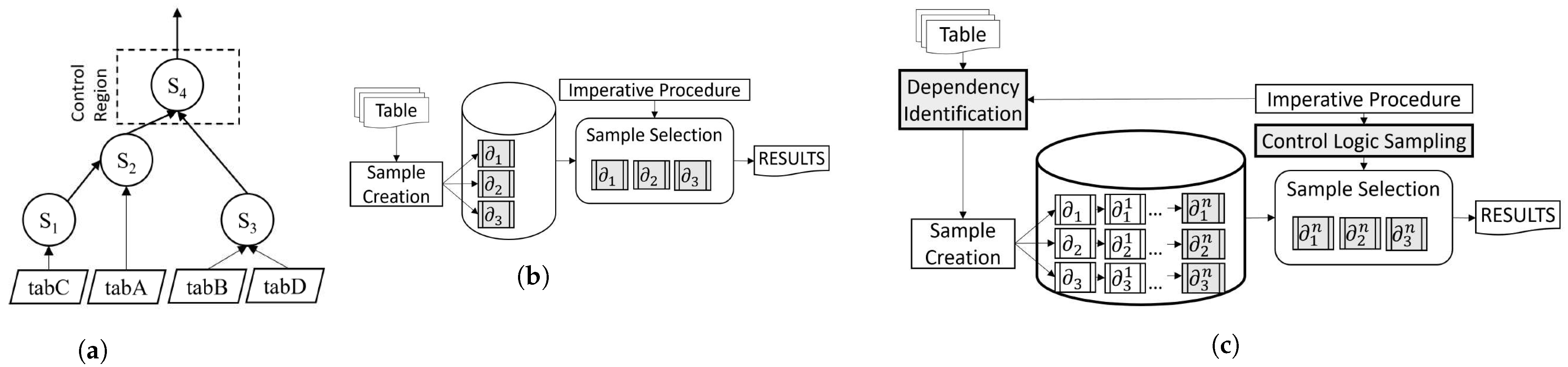

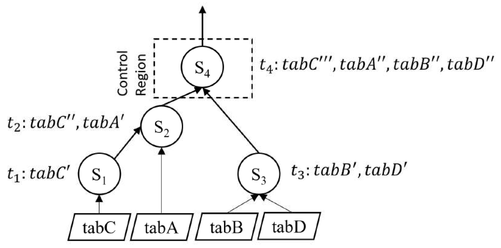
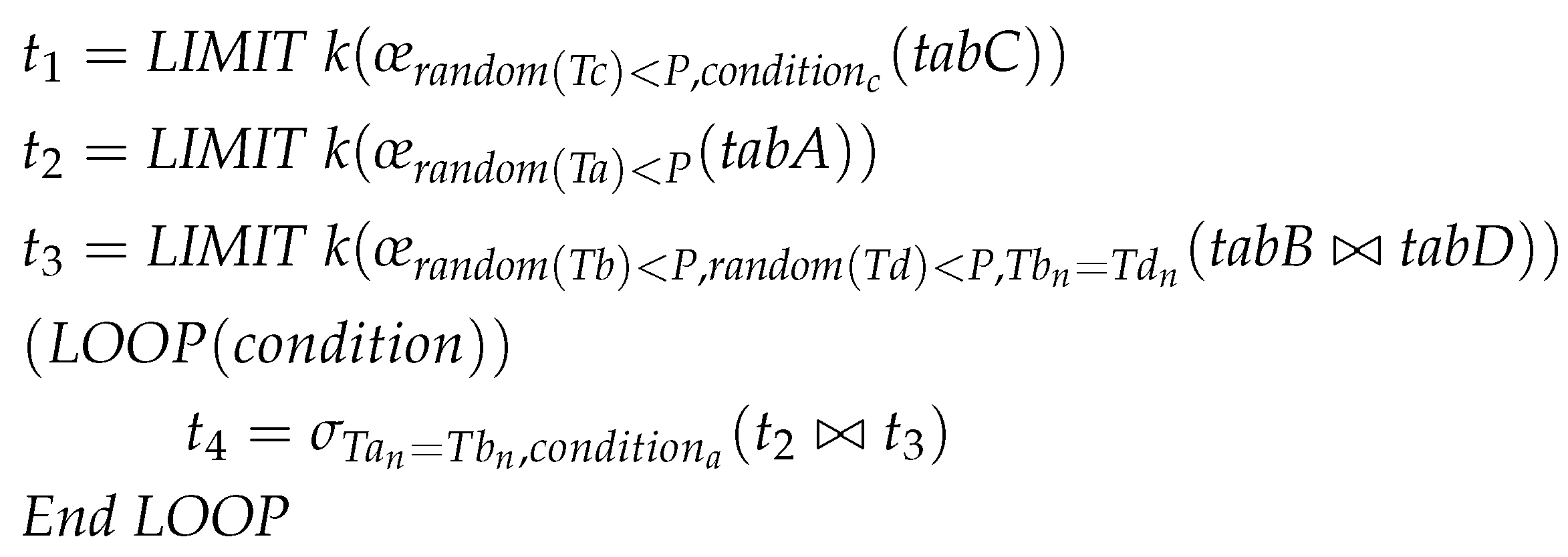

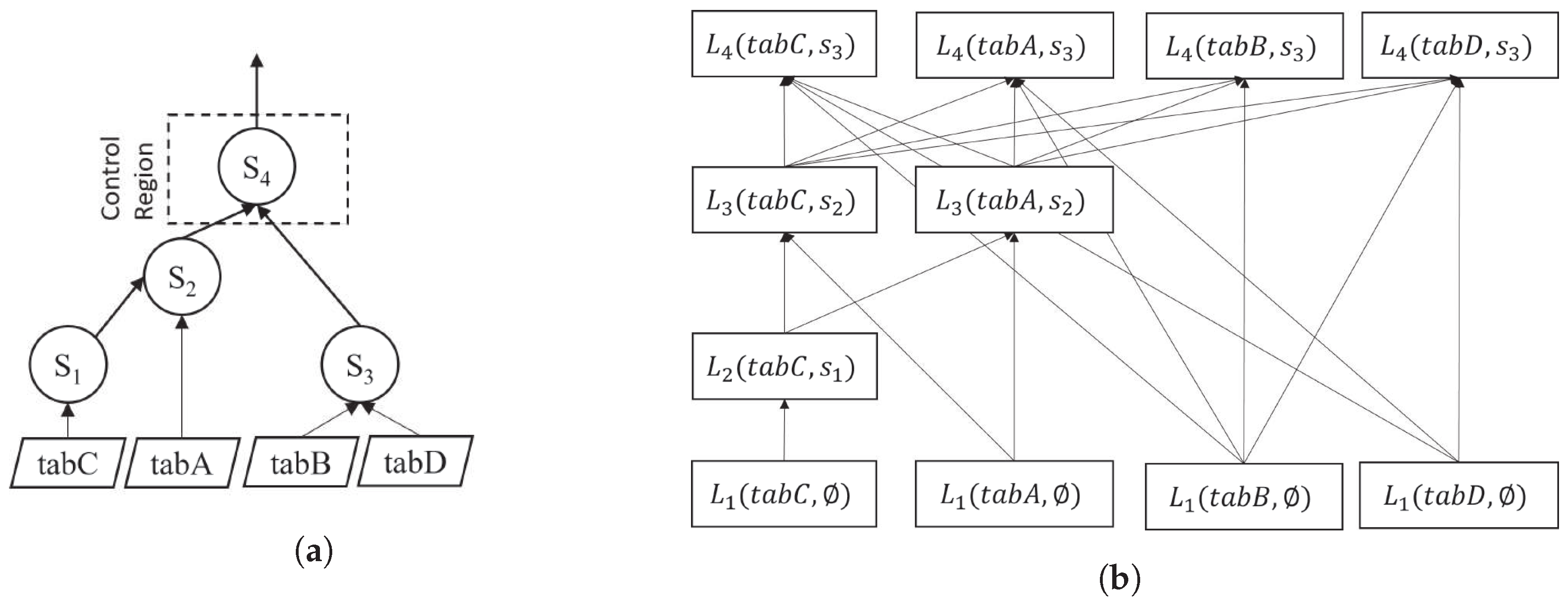
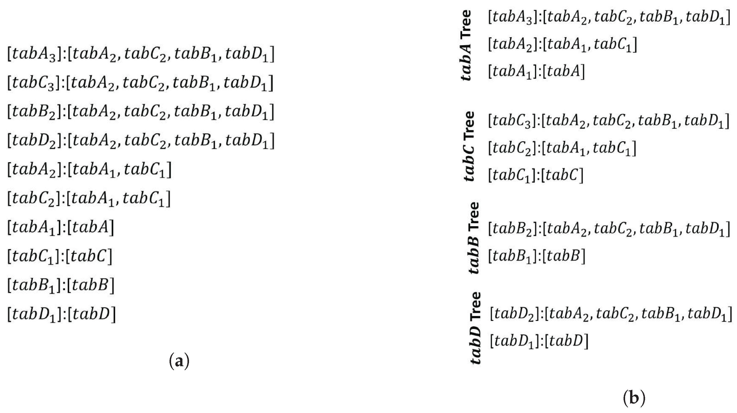

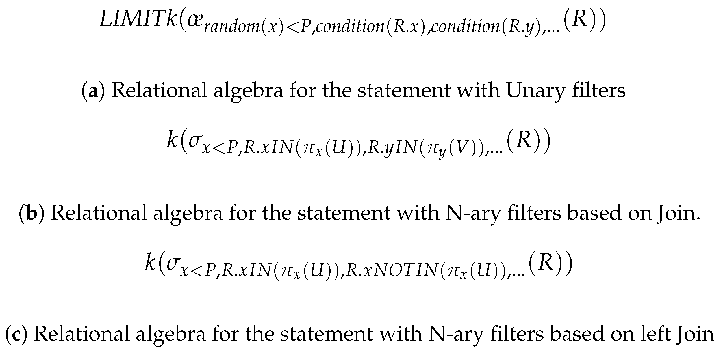


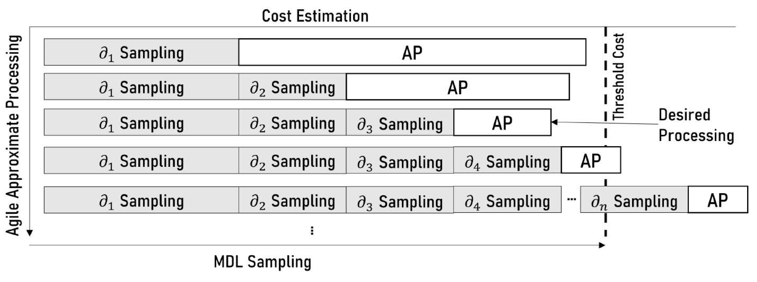


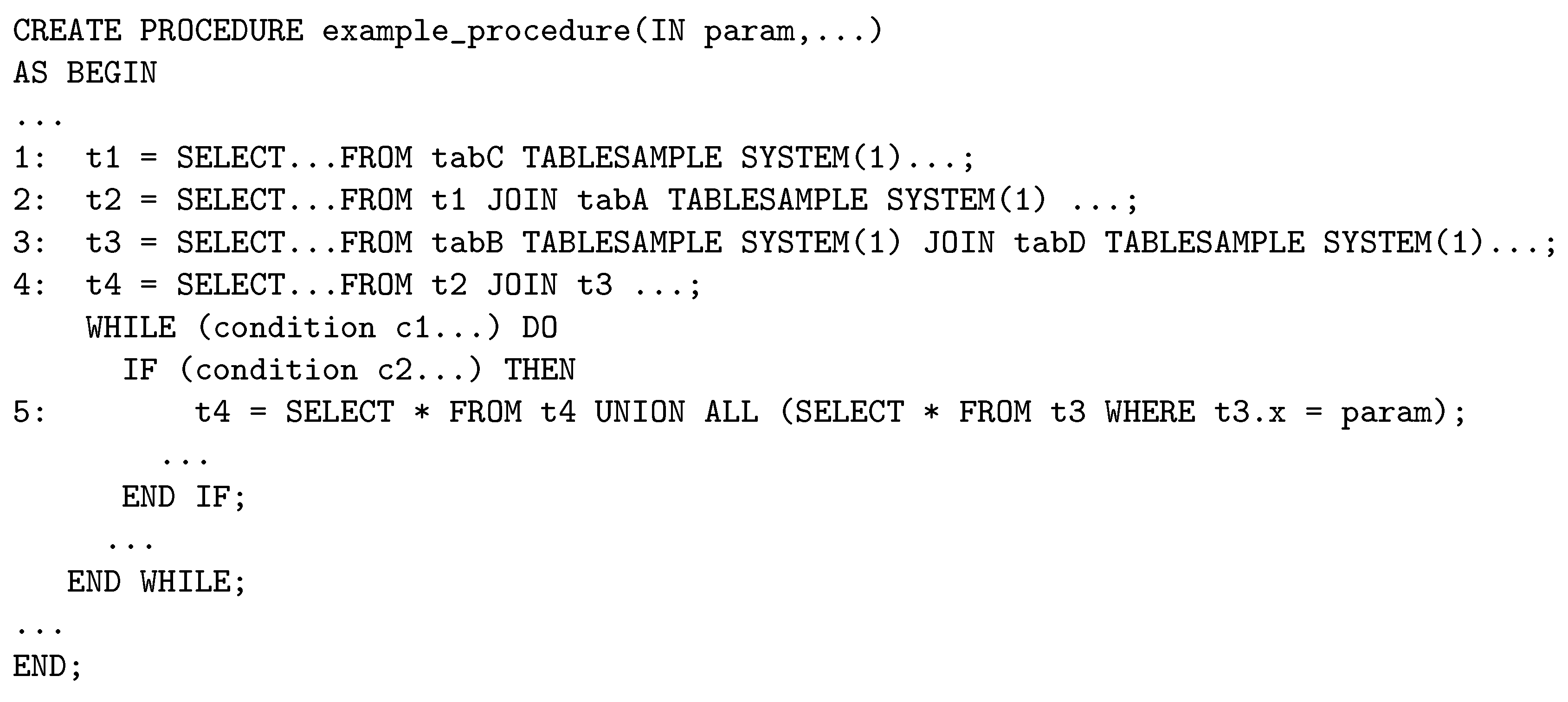
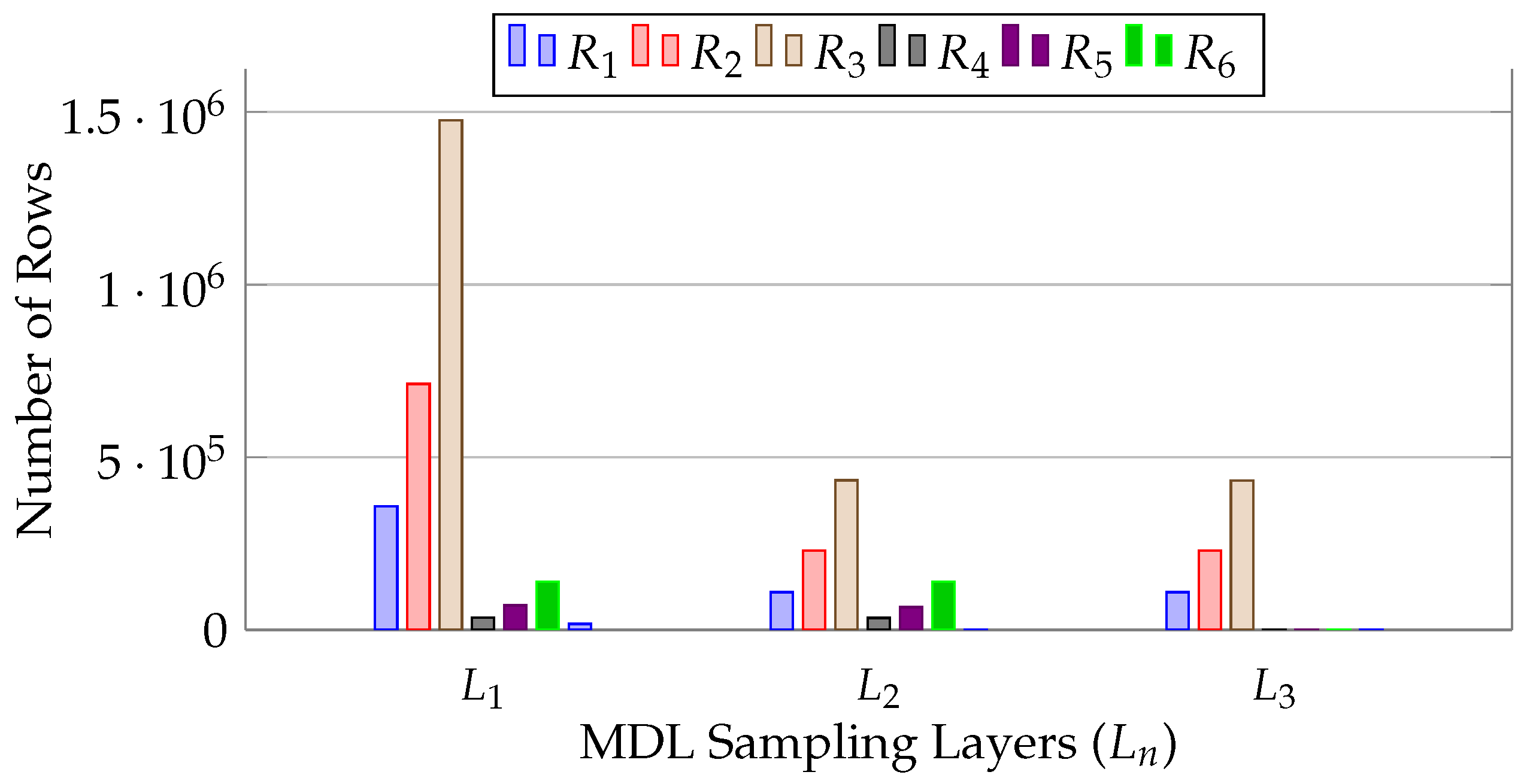
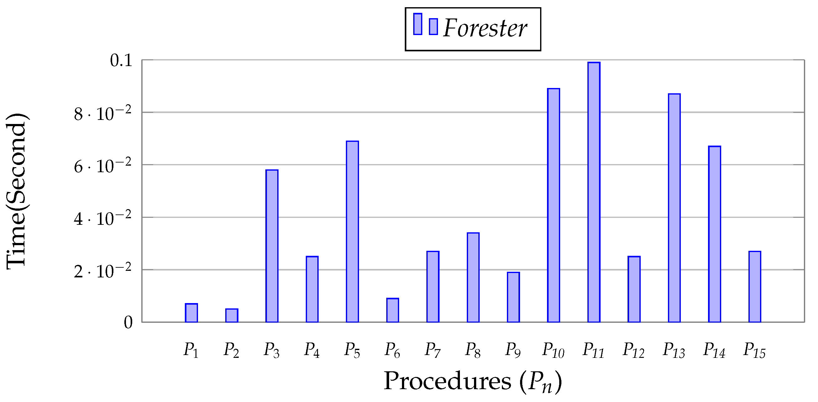
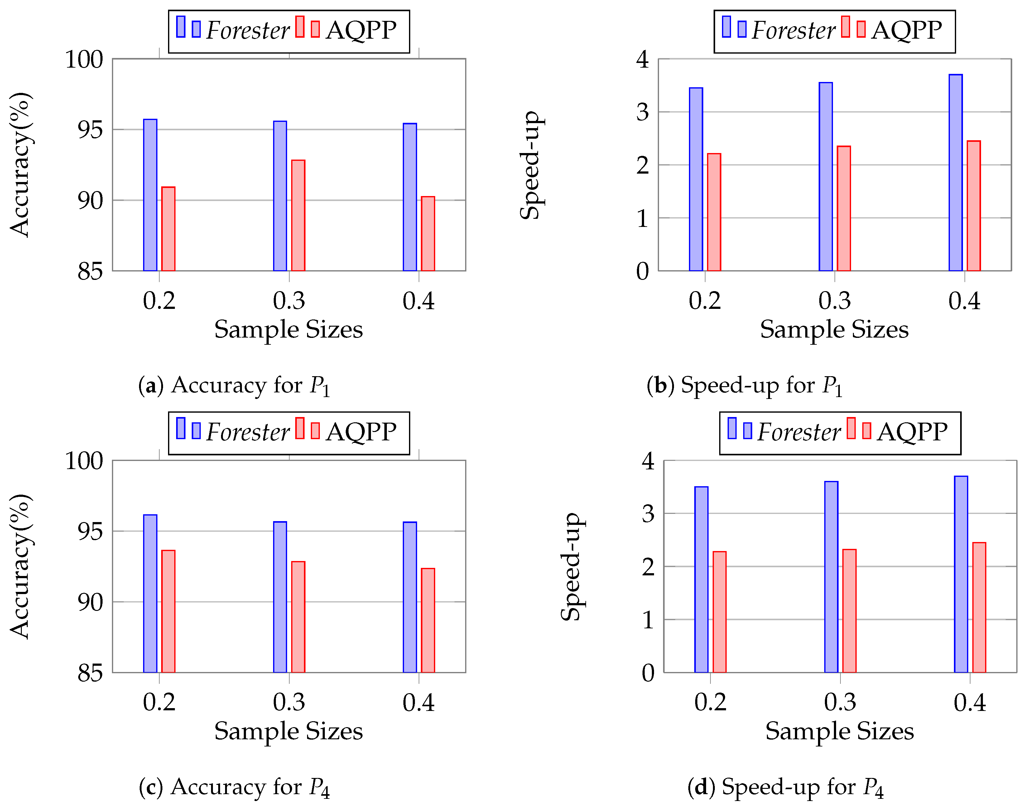
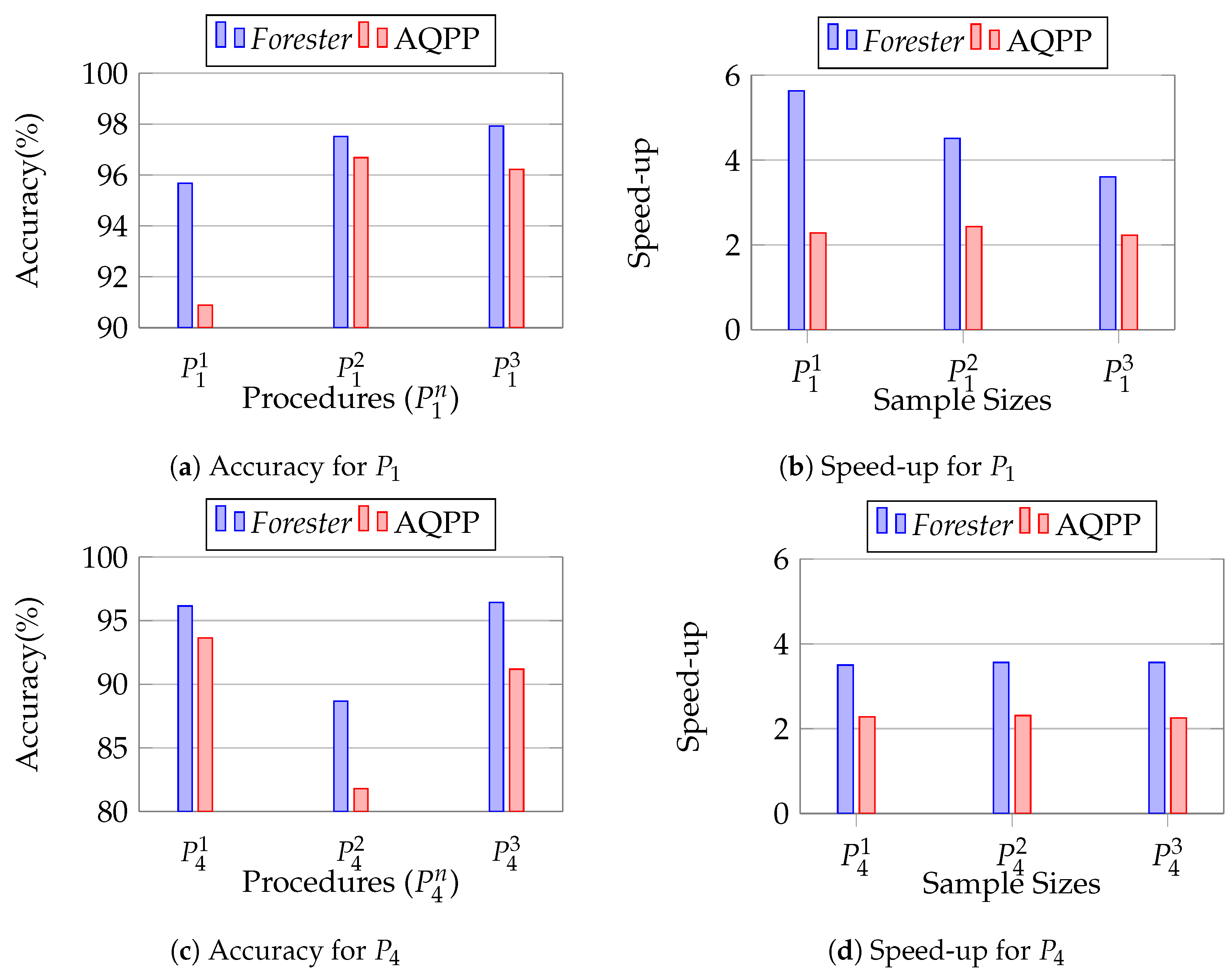
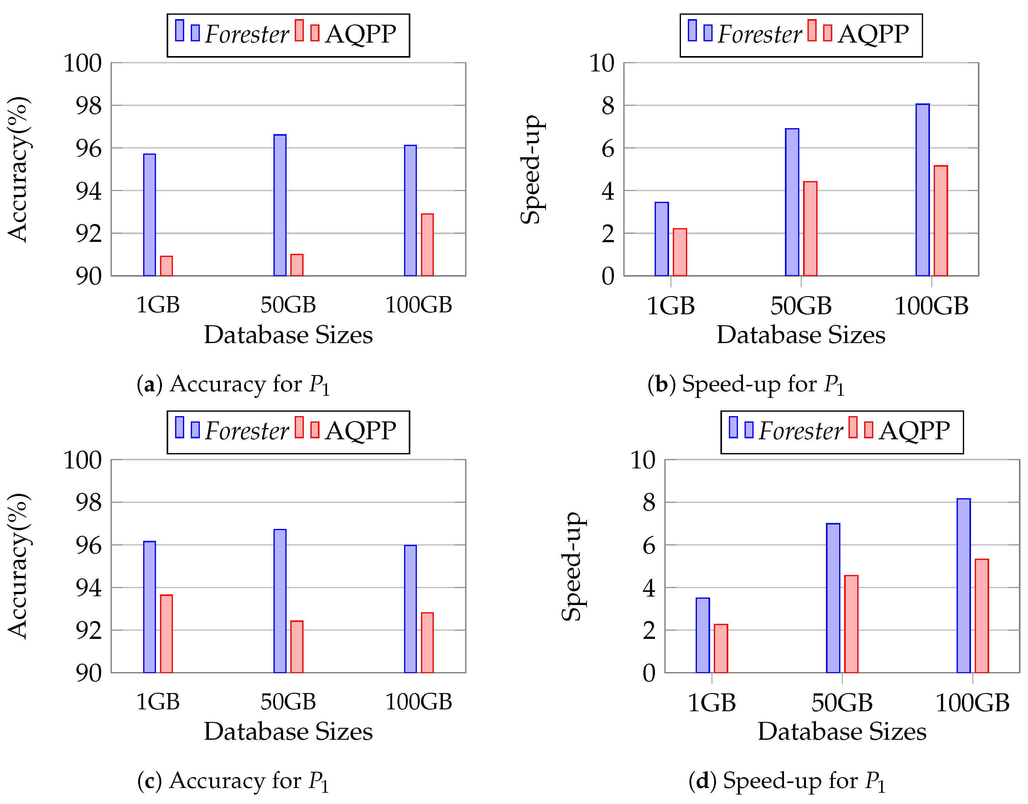
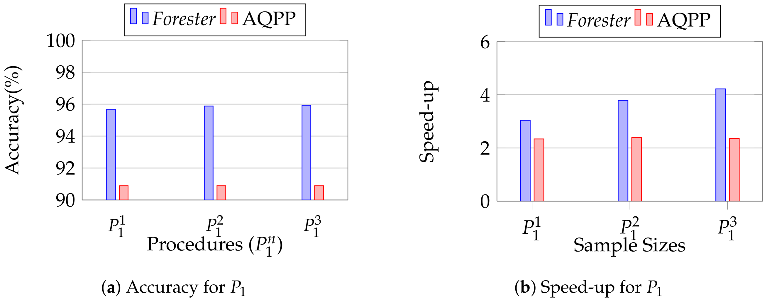
Disclaimer/Publisher’s Note: The statements, opinions and data contained in all publications are solely those of the individual author(s) and contributor(s) and not of MDPI and/or the editor(s). MDPI and/or the editor(s) disclaim responsibility for any injury to people or property resulting from any ideas, methods, instructions or products referred to in the content. |
© 2024 by the authors. Licensee MDPI, Basel, Switzerland. This article is an open access article distributed under the terms and conditions of the Creative Commons Attribution (CC BY) license (https://creativecommons.org/licenses/by/4.0/).