Abstract
Underwater acoustic channels often have to face the interference of impulsive noise, which is usually modeled by α-stable distribution in simulation experiments. To solve the problem of underwater acoustic channel estimation under impulsive noise, this paper proposes a convex combination–variable-step-size least mean p-norm algorithm. The algorithm incorporates a convex combination into the variable-step-size least mean p-norm algorithm and uses the convex combination of different convergence domains provided by changing the parameters of the Gaussian function to further improve the effect after convergence. The simulation results of channel estimation show that the convex combination–variable-step-size least mean p-norm algorithm provides a more stable, robust, and universal solution than the variable-step-size least mean p-norm algorithm.
1. Introduction
In comparison to terrestrial communication, underwater acoustic communication systems often experience greater interference due to the unique characteristics of their environment [1]. One of the most typical sources of interference is the significant amount of pulse noise generated by marine biological activities. Pulse interference refers to irregular pulses or noise peaks that suddenly appear in the communication system, characterized by their discontinuity, substantial amplitude, and short duration. Typically, pulse interference is challenging to effectively eliminate or suppress using filters or other signal processing techniques. This difficulty may lead to signal distortion or difficulty in signal recognition, thereby severely impacting the reliability and accuracy of the communication system.
The significance of channel estimation lies in mitigating distortions and noise caused by the channel in received signals, allowing for the accurate demodulation of data and improving communication performance and spectral efficiency. There are various methods for channel estimation, primarily categorized into those based on reference signals, blind/semi-blind methods, time-domain methods, and frequency-domain methods. Each method has its advantages, drawbacks, and suitable scenarios, requiring selection and design based on the characteristics of the channel and the requirements of the system. To address more complex noise interference in channel estimation, Zhang X et al. proposed a filtering gradient search method based on fractional-order derivatives and linear pre-filtering. The rationality of the proposed algorithm has been demonstrated [2]. In order to enhance the system’s robustness under pulse interference conditions, Zhu Y et al. employed the correlation entropy as a cost function to reduce the system’s sensitivity to pulse interference [3].
Many researchers have integrated deep learning with signal recognition and processing, and empirical evidence has demonstrated the remarkable effectiveness of deep learning in the field of signal processing [4,5,6]. However, deep learning technologies impose high demands on experimental infrastructure, such as a high-quality graphics processing unit, making them inconvenient for use in certain specific scenarios. Therefore, this paper opts for adaptive filtering to process signals.
The most important thing for adaptive algorithms is to choose a cost function, and the least mean square (LMS) algorithm enjoys widespread adoption in engineering applications, this algorithm is favored for its straightforwardness and straightforward implementation [7]. However, using the second-order statistics of the error as the cost function performs poorly in non-Gaussian noise environments and often requires combining other methods to achieve better robustness in practical scenarios with impulsive noise [8,9,10]. There are many marine organisms, such as snapping shrimp, that can emit impulsive noise [11], which causes underwater acoustic channels to be frequently affected by impulsive noise. To make adaptive algorithms more robust under impulsive noise conditions, the least mean p-power (LMP) algorithm is often used to replace the least mean square algorithm [12,13,14]. Xiong K et al., aiming to improve the robustness of adaptive algorithms in the presence of non-linear interference, utilized the minimum average p-norm as a replacement for the traditional minimum mean square error algorithm to upgrade the algorithm. In their paper’s appendix, they provided a comparison of the algorithm’s excess mean square error and mean square deviation (MSD), demonstrating the algorithm’s steady-state performance [15]. Therefore, this paper uses the LMP as the cost function when facing underwater acoustic channels with a lot of non-Gaussian noise.
The variable-step-size algorithm enables the filter to dynamically adjust the step size in response to variations in the error signal; by doing so, it effectively resolves the trade-off between the convergence rate and the quality of convergence, thereby enhancing the algorithm’s overall performance [16,17,18]. Therefore, this paper adopts the variable-step-size least mean p-norm (VSS-LMP) algorithm to implement the estimation of the underwater acoustic channel. However, the traditional variable-step-size algorithm determines the most suitable convergence domain when the variable step-size formula is determined, and the performance often declines when the channel model is changed. Facing different underwater acoustic channels, it is generally necessary to adjust the parameters of the variable-step-size formula to make the algorithm achieve a more satisfactory effect. Therefore, this paper hopes to build a universal algorithm that can achieve a satisfactory effect without adjusting the parameters when facing different channel environments.
The convex combination idea is generally used to balance the advantages and disadvantages of two algorithms. Shi L et al. utilized the maximum correlation entropy criterion when combating pulse interference. To overcome the contradiction between convergence speed and the steady-state mean square, the convex combination concept was employed, leading to a significant improvement in the algorithm’s robustness against pulse noise after the modification [19]. In order to reduce the impact of algorithm parameters on the overall performance, Zhang Y et al. employed the convex combination concept to combine minimum mean square error filters with different parameters. By comparing the excess mean square error in the results, it was observed that the improved algorithm exhibited a noticeable enhancement in performance [20]. In order to address the contradiction between the convergence speed and steady-state error of adaptive filters, Ferrer et al. resolved this issue by convexly combining two different types of minimum mean square error algorithms. They experimentally validated the algorithm’s performance under both steady-state and non-steady-state conditions. The study demonstrated that convex combination could effectively enhance the algorithm’s performance [21]. Based on this, this paper proposes a convex combination–variable-step-size least mean p-norm (CCVSS-LMP) algorithm, which combines two variable-step-size adaptive algorithms with different convergence domains, so that the overall algorithm can achieve better convergence effects without adjusting the parameters when facing different channels. In Section 3 of this paper, the convergence effect of the algorithm is tested, and by comparing the performance of the algorithm in different scenarios, it is found that the proposed algorithm can achieve a relatively ideal convergence effect without changing the parameters when facing different channel environments.
2. CCVSS-LMP Algorithm
Figure 1 shows the system model of the CCVSS-LMP algorithm, where w1(n) and w2(n) are two independent least mean p-norm filters, which jointly estimate the unknown channel w0. In the two filters set in this paper, the update magnitude of w1(n) is larger than that of w2(n).

Figure 1.
System model of the proposed algorithm.
d(n) is the desired signal, as shown in Equation (1), where w0T is the transpose of w0.
The input signal x(n) is as shown in Equation (2), where M is the system length, which refers to the filter length in this paper.
The errors of the two filters w1(n) and w2(n) are e1(n) and e2(n), respectively, and the errors are obtained by Equation (3):
The weight of the whole system w(n) can be seen as Equation (4):
In Equation (4), λn is a scalar between 0 and 1, and the idea is that if λn is given a suitable value each time, the combination will extract the sum of the best attributes of each filter [22]. Since a large step size is needed at the beginning, the initial value of λn is set to 1. And the update formula of λn is as shown in Equation (5), where θλ is the change factor of the λn update formula, which is used to adjust the degree of change each time.
Relative to the weight of the whole system w(n), the error of the whole system e(n) is as shown in Equation (6):
By substituting Equations (3) and (4) into Equation (6), the simplified system error e(n) and the relationship between the errors of the two filters e1(n) and e2(n) are as shown in Equation (7):
To reflect the effect of variable step size, w1(n) and w2(n) adopt the deformed Gaussian function to update the step size [23]. Compared with other step-size update formulas, the deformed Gaussian function has the characteristics of simplicity and efficiency, as shown in Equation (8):
The method frequently employed for forecasting future values is the weighted moving average [24]. To make full use of the correlation between step sizes, this paper employs the moving average technique to adjust the step size and combines the deformed Gaussian function proposed in Equation (8) to obtain the step-size update formulas μ1 and μ2 for the filters w1(n) and w2(n), as shown in Equation (9):
where θ1 and θ2 are independent smoothing factors, which are used to maintain the stability of the algorithm.
The weight update formulas of w1(n) and w2(n) are as shown in Equation (10).
In Equation (10), p is the algorithm norm of LMP.
The algorithm flow of the proposed CCVSS-LMP algorithm is shown in Table 1.

Table 1.
The algorithm flow of CCVSS-LMP.
3. Simulation Analysis of the Proposed Algorithm
To verify the performance of the algorithm, the filter length is set to 256, and the sampling number is 8 × 10⁴. To verify the robustness of the algorithm when the channel changes abruptly, the channel changes at 4 × 10⁴, and the change effect is achieved by inverting the channel in this experiment. The normalized mean square deviation (NMSD) curve is used to measure the performance of the algorithm in this paper [25], which reflects the error between the filter estimate and the actual channel and can intuitively show the convergence effect of the algorithm. The expression is as shown in Equation (11).
The α-stable distribution model is an extension of the Gaussian distribution, applicable to an infinite number of independent and identically distributed random variables with potentially infinite variance; their sum will tend to a stable distribution, which is suitable for modeling the impulsive noise that occurs in underwater acoustic channels [12,26]. The most prominent feature of the α-stable distribution is that the probability distribution function has a heavy tail, and the characteristic function is defined as Equation (12).
In Equation (12), ω(t, α) is defined as in Equation (13), where α is the characteristic exponent, and the range of values is (0,2].
In Equation (12), the sign function sgn(t) is defined as in Equation (14):
Since the second-order statistics no longer converge under α-stable distribution noise, the traditional signal–noise ratio function will lose its meaning under α-stable distribution noise. In order to assess the signal–noise ratio (SNR) of useful signals and pulse noise effectively, it is imperative to employ new methodologies [27]. This paper employs the generalized signal–noise ratio (Formula (15)) in evaluating the system’s signal–noise ratio.
In Equation (15), σs2 denotes the variance of x(n), and γ denotes the scale parameter of the impulsive noise in Equation (12).
3.1. Analysis of Algorithm Parameters
Some parameters are used in this paper, among which the most important one is the selection of the deformed Gaussian function in Equation (8). The Gaussian function is an even function, so only the positive half-axis is considered in the analysis. The function is a unimodal function, and it has output only at the peak position and zero at other positions. Therefore, the algorithm can update its step size and other parameters according to the error only in the peak region, which is the best convergence region of the function. The selection of the variable-step-size parameters α and β in the deformed Gaussian function determines the best convergence region of the Gaussian function. In this paper, the effects of different values of α and β on Equation (8) are compared respectively under the initial values of α = 0.0006 and β = 0.004, as shown in Figure 2 and Figure 3.

Figure 2.
The values of the deformation function under different α.

Figure 3.
The values of the deformation function under different β.
As shown in Figure 2, the output increases with an increase in α for the same input, which means that the filter can provide larger feedback for the same error input. We hope that the algorithm can produce fast feedback to the error in the initial stage of the filter. Since w1(n) has a faster update speed by default in this paper, the setting of α for w1(n) should be larger than that for w2(n).
As shown in Figure 3, the output decreases with an increase in β for the same input, and the input corresponding to the output peak also decreases continuously, which means that only small input can affect the output. In order to make w2(n) have a smaller step-size update and achieve a better steady-state effect, the setting of β for w2(n) should be larger than that for w1(n).
Due to the faster step-size update of the filter w1(n) than that of w2(n), θ1 should be smaller than θ2. Through extensive experiments, we found that the ideal effect can be obtained when θ1 is between 0.8 and 0.9 and θ2 is between 0.9 and 1.0. In the experiments of this paper, the smoothing factors are set as θ1 = 0.85 and θ2 = 0.98.
3.2. Simulation Channel Analysis and Analysis of Parameters of the Algorithm
This paper first analyzes the unknown system using simulation. The channel and the two filters w1(n) and w2(n) of the unknown system follow a Gaussian distribution with zero mean and unit variance. The parameters of the experiment are set as follows: α1 = 0.00059, β1 = 0.0049, α2 = 0.00032, β2 = 0.0049, θλ = 0.0004, p = 1.15, and α-stable distribution parameters α = 1.45 and γ = 0.039. The impulse noise image is shown in Figure 4; noise signals are introduced into the adaptive algorithm in an additive manner, and v(n) in Equation (1) represents the impulse noise added to the system. The performance comparison of CCVSS-LMP and pre-combination algorithm are shown in Figure 5.

Figure 4.
Image of impulse noise in the system.

Figure 5.
Performance comparison of CCVSS-LMP and pre-combination algorithm.
In Figure 5, LMP1 and LMP2 are independent algorithms before convex combination, where LMP1 and w1(n) have the same parameter settings, and LMP2 and w2(n) have the same parameter settings. Through simulation experiments, it can be found that under the same number of iterations, the performance of the proposed CCVSS-LMP algorithm is significantly better than that of the improved algorithm, and it can still maintain the convergence effect of the original algorithm after the system undergoes mutation.
Figure 6 shows the curve of the change in λn, and it can be seen that λn starts from 1 initially and always shows a downward trend with a change in the number of iterations and can still continue to maintain the downward trend from 1 to 0 after the system undergoes mutation, which is consistent with the expectation for λn.

Figure 6.
The variation curve of λn parameter value.
In order to balance each experiment and ensure that the experimental results are not affected by some special cases, 100 independent Monte Carlo simulations are used to compare the algorithms, and the average values of NMSD and λn are obtained at the end [28]. The simulation results are shown in Figure 7 and Figure 8. From Figure 7, it can be seen that after excluding the interference of accidental situations, the proposed algorithm still outperforms the improved algorithm. From Figure 8, it can be seen that as the algorithm iterates, λn can always drop to a value close to 0, which is consistent with the overall expectation for the algorithm.

Figure 7.
Comparison of algorithms based on Monte Carlo simulation.

Figure 8.
λn value variation curve based on Monte Carlo simulation.
The same parameters may not be suitable for all algorithms, and it is easier to compare the advantages of the proposed algorithm by comparing it with the improved-parameter algorithm [29]. Under the same simulation conditions, it is compared with the VSS-LMP, the LMS, and the convex combination–least mean square (CC-LMS) algorithm, where the step size of LMS is set to 0.005, the step size of CC-LMS is set to 0.001 and 0.0001, and the α, β, and θ of VSS-LMP are set to 0.0006, 0.004, and 0.98, respectively, and Figure 9 is obtained.

Figure 9.
Comparison of different algorithms in simulation channel.
By analyzing Figure 9, it can be found that under the same simulation environment, the proposed algorithm can obtain faster convergence speed and lower error after convergence than the ordinary VSS-LMP algorithm by convex combination. By comparing with the LMS and CC-LMS algorithms, it can be observed that the least mean squares (LMS) algorithm exhibits suboptimal performance in the context of an underwater acoustic channel, particularly in the presence of impulse interference. Even if the LMS algorithm is improved by the convex combination method, it is still difficult to achieve an ideal convergence effect. And the proposed algorithm has a significant bending curvature when the iteration number reaches approximately 42,900 after the channel undergoes mutation, which is consistent with the effect shown in other convex combination algorithms.
To further compare the impact of algorithm parameters on the convergence effect, we conducted an ablation study on the proposed CCVSS-LMP algorithm. Contrasting the algorithm under different parameter settings allows for an intuitive demonstration of the roles played by these parameters in the algorithm.
In this paper, we first compared the impact of different values of θ on the algorithm, as illustrated in Figure 10 and Figure 11.

Figure 10.
The impact of the value of θ1 on the algorithm.
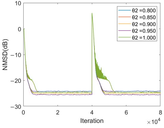
Figure 11.
The impact of the value of θ2 on the algorithm.
Analysis of Figure 10 reveals that θ1 has a relatively minor impact on the algorithm, primarily affecting the computational iterations required for the convergence inflection point of the convex combination, with little influence on the final steady-state convergence effect. Analysis of Figure 11 indicates that θ2 primarily affects the steady-state error reached after convergence. When θ2 is less than 1, the steady-state error gradually decreases with an increase in θ2 in the algorithm.
By analyzing Figure 12 and Figure 13, it is observed that with a gradual increase in α1, at a low number of iterations, lower NMSD can be achieved at the same iteration count, but the arrival time of the inflection point becomes earlier. Similarly, for β1, it also affects the algorithm’s early-stage convergence speed. Both α1 and β1 influence the early-stage convergence speed, while their impact on the final convergence error can be neglected. This aligns with the design intention of filter w1 to enhance the convergence speed.

Figure 12.
The impact of the value of α1 on the algorithm.

Figure 13.
The impact of the value of β1 on the algorithm.
Through the analysis of Figure 14, it is observed that as the parameter α2 decreases, the steady-state error after algorithm convergence increases. Analyzing Figure 15 reveals that with a decrease in parameter β2, the NMSD after reaching steady-state becomes larger. At β2 = 0.009, when facing channel mutations, the algorithm exhibits suboptimal early-stage convergence (spikes appearing between iterations 42,000–44,000). Therefore, the value of β2 should not be excessively large. Comparing Figure 14 and Figure 15, it can be seen that the impact of α2 and β2 values on early-stage convergence speed is not significant; the inflection points of the algorithm occur almost at the same iteration count. However, there is a significant correlation between these parameters and the steady-state error after algorithm convergence, aligning with the original intent of designing filter w2 to enhance the overall reliability of the algorithm.

Figure 14.
The impact of the value of α2 on the algorithm.
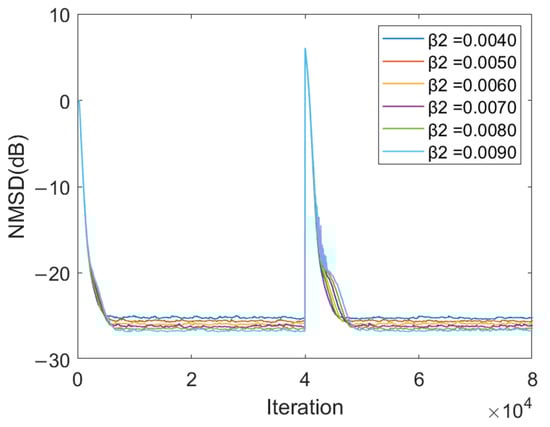
Figure 15.
The impact of the value of β2 on the algorithm.
3.3. Real Channel Analysis
To investigate the efficacy of the CCVSS-LMP algorithm in an authentic underwater acoustic channel, this section compares the proposed algorithm with an actual channel. Under impulse interference, this section uses the measured impulse response of a channel in the Norwegian sea area at a certain moment as the weight vector w0 for identification [30] and simulates the estimation performance of each algorithm, where the parameters of the proposed algorithm are consistent with those in the simulation channel experiment. Figure 16 shows the impulse response of the authentic underwater acoustic channel.

Figure 16.
Impulse response of authentic underwater acoustic channel.
Figure 17 shows the performance of the CCVSS-LMP algorithm and the improved algorithm in the authentic underwater acoustic channel, where LMP1 and LMP2 are the two algorithms before convex combination under the same parameters. Comparing Figure 17, it can be found that the proposed CCVSS-LMP algorithm can greatly improve the convergence effect of the algorithm in the authentic underwater acoustic channel environment by the convex combination improvement.

Figure 17.
Comparison of the algorithm before and after the improvement in the authentic channel.
The above comparison only compares the convergence effects of filters with the same parameters. To further assess the proposed algorithm, it is compared with alternative algorithms in the authentic channel environment, where the step size of CC-LMS is reduced to 0.0008 and 0.00001 to improve the effect after convergence, as shown in Figure 18.

Figure 18.
Comparison of the proposed algorithm with other algorithms in real channels.
By analyzing Figure 18, it can be found that CCVSS-LMP still has faster convergence speed and smaller error after convergence in the real channel environment, facing impulse interference. When the step size is further reduced, CC-LMS still has difficulty in obtaining the ideal convergence effect in the authentic underwater environment under impulsive interference.
By increasing the SNR from 15 dB to 25 dB, Figure 19 was obtained. Through the analysis of Figure 19, it can be observed that with the improvement in SNR, the steady-state error achieved by the algorithm after convergence further decreases. Under the same number of iterations, the proposed algorithm consistently achieves lower steady-state errors after convergence.

Figure 19.
Comparison of the algorithms at a SNR of 25 dB in real channel.
3.4. Measured Channel Analysis
In order to study the performance of the proposed algorithm in different underwater acoustic channels, we measured the channel information of a reservoir in Zhenjiang. Figure 20 shows the measured impulse response of the underwater acoustic channel of the reservoir. The parameters of CCVSS-LMP remain unchanged. The step size of LMS is set to 0.004, the step size of CC-LMS is set to 0.004 and 0.0001, and the α, β, and θ of VSS-LMP are set to 0.00045, 0.001, and 0.98 respectively. The comparison results are shown in Figure 21.

Figure 20.
Impulse response of measured underwater acoustic channel.

Figure 21.
Comparison of the proposed algorithm with other algorithms in measured channel.
As shown in Figure 21, the proposed algorithm can achieve good convergence performance in different channel environments, and compared with other algorithms, the proposed algorithm does not need to modify the parameters to achieve a good convergence effect. Due to the impact of impulsive noise, the LMS algorithm and the CC-LMS algorithm still cannot obtain an ideal convergence effect in the new underwater acoustic channel.
In the practical measurement of the channel, we obtain Figure 22 by increasing the signal–noise ratio (SNR) from 15 dB to 25 dB. Through the analysis of Figure 22, it can be observed that with an improvement in SNR, the NMSD after the convergence of the algorithm decreases by approximately 24 dB. Furthermore, the proposed CCVSS-LMP algorithm still exhibits faster convergence speed and better convergence performance.

Figure 22.
Comparison of the algorithms at a SNR of 25 dB in measured channel.
4. Conclusions
In this paper, in the background of using α-stable noise as impulse interference, in order to further improve the convergence effect of an existing algorithm for an underwater acoustic channel, based on the variable VSS-LMP algorithm, the convex combination is used to improve it, and two sub-filters with different convergence domains are combined; hence, a novel algorithm is introduced, namely the convex combination–variable-step-size least mean p-norm algorithm, designed to exhibit resilience against impulsive noise. Through experiments in a simulation channel, a real channel, and a measured channel, it can be found that CCVSS-LMP demonstrates accelerated convergence and diminished steady-state error when facing impulsive noise and can achieve a better convergence effect than VSS-LMP in different environments without the need to modify the parameters. In summary, the proposed algorithm in this paper has better stability, robustness, and universality.
Author Contributions
Methodology, B.Z. and B.C.; software, B.Z.; formal analysis, B.Z., B.C., B.W., and Y.Z.; data curation, B.Z., B.W., and Y.Z.; writing—original draft preparation, B.Z. and B.W.; writing—review and editing, B.Z. and B.W.; funding acquisition, B.W. All authors have read and agreed to the published version of the manuscript.
Funding
This work was supported in part by the National Natural Science Foundation of China under Grant 52071164 and in part by the Postgraduate Research & Practice Innovation Program of Jiangsu Province under Grant KYCX23_3877.
Data Availability Statement
Data are obtained within the article.
Conflicts of Interest
The authors declare no conflicts of interest.
Abbreviations
Many abbreviations are quoted in the paper, and their meanings are explained here.
| Abbreviation | Full Name |
| LMS | least mean square |
| LMP | least mean p-power |
| VSS-LMP | variable-step-size least mean p-power |
| CCVSS-LMP | convex combination–variable-step-size least mean p-norm |
| NMSD | normalized mean square deviation |
| CC-LMS | convex combination–least mean square |
References
- Chitre, M. A high-frequency warm shallow water acoustic communications channel model and measurements. J. Acoust. Soc. Am. 2007, 122, 2580–2586. [Google Scholar] [CrossRef]
- Zhang, X.; Ding, F. Optimal Adaptive Filtering Algorithm by Using the Fractional-Order Derivative. IEEE Signal Process. Lett. 2021, 29, 399–403. [Google Scholar] [CrossRef]
- Zhu, Y.; Zhao, H. A Robust Generalized Maximum Correntropy Criterion Algorithm for Active Noise Control. IFAC-PapersOnLine 2019, 52, 299–303. [Google Scholar] [CrossRef]
- Wang, H.; Wang, B.; Li, Y. IAFNet: Few-Shot Learning for Modulation Recognition in Underwater Impulsive Noise. IEEE Commun. Lett. 2022, 26, 1047–1051. [Google Scholar] [CrossRef]
- Mustaqeem Ishaq, M.; Kwon, S. A CNN-Assisted deep echo state network using multiple Time-Scale dynamic learning reservoirs for generating Short-Term solar energy forecasting. Sustain. Energy Technol. Assess. 2022, 52, 102275. [Google Scholar] [CrossRef]
- Li, Y.; Wang, B.; Shao, G.; Shao, S.; Pei, X. Blind Detection of Underwater Acoustic Communication Signals Based on Deep Learning. IEEE Access 2020, 8, 204114–204131. [Google Scholar] [CrossRef]
- Al-Sayed, S.; Zoubir, A.M.; Sayed, A.H. Robust Adaptation in Impulsive Noise. IEEE Trans. Signal Process. 2016, 64, 2851–2865. [Google Scholar] [CrossRef]
- Zhang, S.; Zhang, J.; Han, H. Robust Variable Step-Size Decorrelation Normalized Least-Mean-Square Algorithm and Its Application to Acoustic Echo Cancellation. IEEE/ACM Trans. Audio Speech Lang. Process. 2016, 24, 2368–2376. [Google Scholar] [CrossRef]
- Hajiabadi, M.; Radmanesh, H.; Samkan, M. Robust adaptive beamforming in impulsive noise environments. IET Radar Sonar Navig. 2019, 13, 2145–2150. [Google Scholar] [CrossRef]
- Li, L.; Zhao, H. A Robust Total Least Mean M-Estimate Adaptive Algorithm for Impulsive Noise Suppression. IEEE Trans. Circuits Syst. II 2020, 67, 800–804. [Google Scholar] [CrossRef]
- Au, W.W.L.; Banks, K. The acoustics of the snapping shrimp Synalpheus parneomeris in Kaneohe Bay. J. Acoust. Soc. Am. 1998, 103, 41–47. [Google Scholar] [CrossRef]
- Shao, M.; Nikias, C.L. Signal processing with fractional lower order moments: Stable processes and their applications. Proc. IEEE 1993, 81, 986–1010. [Google Scholar] [CrossRef]
- Arikan, O.; Enis Cetin, A.; Erzin, E. Adaptive filtering for non-Gaussian stable processes. IEEE Signal Process. Lett. 1994, 1, 163–165. [Google Scholar] [CrossRef]
- Luo, Y.; Yang, J.; Zhang, Q.; Wang, C. A Fractional-Order Adaptive Filtering Algorithm in Impulsive Noise Environments. IEEE Trans. Circuits Syst. II 2021, 68, 3376–3380. [Google Scholar] [CrossRef]
- Xiong, K.; Zhang, Y.; Wang, S. Robust variable normalization least mean p-power algorithm. Sci. China Inf. Sci. 2020, 63, 199204. [Google Scholar] [CrossRef]
- Harris, R.; Chabries, D.; Bishop, F. A variable step (VS) adaptive filter algorithm. IEEE Trans. Acoust. Speech Signal Process. 1986, 34, 309–316. [Google Scholar] [CrossRef]
- Vega, L.R.; Rey, H.; Benesty, J.; Tressens, S. A New Robust Variable Step-Size NLMS Algorithm. Trans. Signal Process. 2008, 56, 1878–1893. [Google Scholar] [CrossRef]
- Paleologu, C.; Ciochina, S.; Benesty, J. Variable Step-Size NLMS Algorithm for Under-Modeling Acoustic Echo Cancellation. IEEE Signal Process. Lett. 2008, 15, 5–8. [Google Scholar] [CrossRef]
- Shi, L.; Lin, Y. Convex Combination of Adaptive Filters under the Maximum Correntropy Criterion in Impulsive Interference. IEEE Signal Process. Lett. 2014, 21, 1385–1388. [Google Scholar] [CrossRef]
- Zhang, Y.; Chambers, J.A. Convex Combination of Adaptive Filters for a Variable Tap-Length LMS Algorithm. IEEE Signal Process. Lett. 2006, 13, 628–631. [Google Scholar] [CrossRef]
- Ferrer, M.; Gonzalez, A.; De Diego, M.; Pinero, G. Convex Combination Filtered-X Algorithms for Active Noise Control Systems. IEEE Trans. Audio Speech Lang. Process. 2013, 21, 156–167. [Google Scholar] [CrossRef]
- Arenas-García, J.; Figueiras-Vidal, A.; Sayed, A. Mean-square performance of a convex combination of two adaptive filters. IEEE Trans. Signal Process. 2006, 54, 1078–1090. [Google Scholar] [CrossRef]
- Biao, W.; Hanqiong, L.I.; Gao, S.; Mingliang, Z.; Chen, X.U. A Variable Step Size Least Mean p-Power Adaptive Filtering Algorithm. JEIT 2022, 44, 661–667. [Google Scholar]
- Hansun, S. A new approach of moving average method in time series analysis. In Proceedings of the 2013 Conference on New Media Studies (CoNMedia), Tangerang, Indonesia, 27–28 November 2013; pp. 1–4. [Google Scholar]
- Lee, M.; Park, T.; Park, P. Variable Step-Size l0-Norm Constraint NLMS Algorithms Based on Novel Mean Square Deviation Analyses. IEEE Trans. Signal Process. 2022, 70, 5926–5939. [Google Scholar] [CrossRef]
- Qiu, T.S.; Yang, Z.C.; Li, X.B.; Chen, Y.X. A weighted average least p-norm algorithm under alpha stable noise conditions. J. Electron. Inf. 2007, 29, 410–413. [Google Scholar]
- Li, J.; Feng, D.Z.; Li, B. A robust adaptive weighted constant modulus algorithm for blind equalization of wireless communications systems under impulsive noise environment. AEU—Int. J. Electron. Commun. 2018, 83, 150–155. [Google Scholar] [CrossRef]
- Zhu, L.; Song, C.; Pan, L.; Li, J. Adaptive Filtering Under the Maximum Correntropy Criterion with Variable Center. IEEE Access 2019, 7, 105902–105908. [Google Scholar] [CrossRef]
- Zhu, B.; Wang, B.; Cai, B.; Zhu, Y.; Chao, P.; Fang, Z. A variable step size least mean p-power adaptive filtering algorithm based on multi-moment error fusion. EURASIP J. Adv. Signal Process. 2023, 2023, 77. [Google Scholar] [CrossRef]
- van Walree, P.; Otnes, R.; Jenserud, T. Watermark: A realistic benchmark for underwater acoustic modems. In Proceedings of the 2016 IEEE Third Underwater Communications and Networking Conference (UComms), Lerici, Italy, 30 August–1 September 2016; pp. 1–4. Available online: https://ieeexplore.ieee.org/document/7583423 (accessed on 16 December 2023).
Disclaimer/Publisher’s Note: The statements, opinions and data contained in all publications are solely those of the individual author(s) and contributor(s) and not of MDPI and/or the editor(s). MDPI and/or the editor(s) disclaim responsibility for any injury to people or property resulting from any ideas, methods, instructions or products referred to in the content. |
© 2024 by the authors. Licensee MDPI, Basel, Switzerland. This article is an open access article distributed under the terms and conditions of the Creative Commons Attribution (CC BY) license (https://creativecommons.org/licenses/by/4.0/).