Flexible Approach for the Generation of Macro-Basis Functions Using the Characteristic Basis Function Method

Abstract

This document presents a method for reducing the memory and CPU time required for the electromagnetic analysis of complex scenarios employing the Characteristic Basis Function Method. This technique introduces a novel procedure to accelerate the calculation of basis functions and the reduced matrix. The accuracy and computational cost associated with this approach are studied and validated through a number of test cases, making use of about five times less memory than with the conventional approach.

1. Introduction

The method of moments (MoM) [1] is widely regarded as a cornerstone for the electromagnetic analysis of applications related to a wide range of industrial sectors. However, the conventional MoM may present serious computational difficulties for problems of moderate size or complexity because it requires the computation and storage of the impedance matrix between every basis and testing function. Due to this drawback, it is common to make use of either hybrid approaches [2,3,4,5] or efficient modifications to the conventional MoM that avoid handling the full impedance matrix.

The Adaptive Cross Approximation (ACA) [6,7], for example, avoids the computation of the full MoM impedance matrix by storing instead a compressed block-wise approximation, taking advantage of the rank-deficient characteristics of the far-field impedance submatrices. A similar strategy is used in [8], which makes use of a dual modified Gram–Schmidt block QR factorization based on a low-rank singular value decomposition, or the Matrix Decomposition Algorithm, outlined in [9].

Many other approaches make use of an efficient evaluation of the matrix–vector products performed in an iterative solution stage that precludes storing the full impedance matrix and only requires the compact storage of some of its coefficients. The Complex Multipole Beam Approach (CMBA) [10], the Adaptive Integral Method (AIM) [11] and the Impedance Matrix Localization technique (IML) [12] are some approaches that follow this strategy. However, the Multilevel Fast Multipole Method (MLFMM) [13] is probably the most well-known method that falls into this category, requiring the computation of only the near-field part of the impedance matrix after partitioning the computational space in terms of regions with a typical size of 0.25 wavelengths, which are grouped into higher-level regions following an octal tree distribution. The matrix–vector products are then taken by means of the aggregation, translation and disaggregation of the fields due to the basis functions contained in these regions. Additionally, the MLFMM presents good scalability properties for the analysis of large problems using shared or distributed memory systems as well as Graphic Processing Units (GPUs) [14,15,16].

Other approaches increase the efficiency of the analysis by reducing the number of unknowns. For this purpose, a new set of macro-basis functions (MBFs) is computed in a preprocessing stage, replacing the subdomain-type functions used in conventional approaches. The MBFs extend over geometrical blocks with typical sizes of one to a few wavelengths. The Synthetic Function Expansion technique (SFX) [17] and the Characteristic Basis Function Method (CBFM) [18,19,20,21,22,23] are known MBF-based approaches. Note that the use of macro-basis functions is in general compatible with other fast methods. The MBFs can be generated using a variety of approximations, including MoM and Physical Optics (PO) [19] and the inclusion of fast ray-tracing-based techniques to further reduce the number of MBFs [20]. The CBFM is combined with the MLFMM in [21], where, for very large problems only, the matrix coefficients between macro-basis functions defined on the same or neighboring blocks are computed and stored, and conventional multipole expansions are modified in order to be adapted to multipole expansions associated with these macro-basis functions. The CBFM is combined with the ACA to analyze large antenna arrays in [22], introducing a scheme for the generation of basis functions that do not conform to the edge condition at the truncated edge of each block. A fast method for the generation of macro-basis functions of progressively larger blocks following a multilevel approach is presented in [23]. A special treatment in the generation of macro-basis functions focused on the improvement of convergence is applied in [24].

As indicated above, the generation of MBFs involves additional preprocessing time since such functions are tailored to the geometry contained in the block or domain over which they are defined. However, the computation of each MBF set is independent from the rest, which favors the scalability of this process when using large computing clusters. The memory footprint required for the storage of the MBFs and the reduced matrix can be very important for large problems and, in some instances, can be a limiting factor regarding the size of the cases that can be addressed.

This work introduces new MBFs that are much faster to compute than those using conventional full-wave techniques, allowing for an increase in the block size in order to reduce the total number of unknowns without suffering a noticeable computational burden. A distance parameter is defined to determine a threshold used to retain coupling data for the generation of the MBFs. In addition, a pseudoinverse matrix is used in order to accelerate the computation of currents induced by a large number of excitations around each block, which are then used to extract the MBFs. These modifications allow us to greatly reduce the memory requirements, increasing the size of the problems that can be analyzed. Note that the CBFM is very well suited to monostatic RCS problems, where it is common to solve the system for hundreds or even thousands of incident directions, and, in such cases, the solution time exceeds by far the preprocessing time. For cases with a moderate number of incident directions, the preprocessing time can represent a noticeable part of the total simulation time, and the CPU time improvement obtained with the presented approach can be very substantial. The main contributions described in this work can be outlined as follows: (i) the application of an efficient MLFMM-CBFM approach where a sparse version of the coupling matrix of each block is used both for the CBF generation and for the computation of the reduced matrix and (ii) the generation of a sparse approximate inverse matrix of the previously sparsified reduced matrix, allowing for the direct computation of current solutions for a very large number of excitations on each block. The document is arranged as follows: Section 2 presents some fundamental ideas about the proposed technique. Section 3 presents, in turn, specific details regarding the proposed improvements for the generation of the MBFs for each block. This approach is validated in Section 4 using some representative test cases. Finally, Section 5 presents some conclusions obtained from this work.

2. Electromagnetic Kernel

The CBFM relies on the substitution of the conventional MoM basis functions with a new set of macro-basis functions, called Characteristic Basis Functions (CBFs) in this context. The conventional MoM basis functions will be referred to as low-level basis functions in this work in order to emphasize the distinction with respect to the CBFs.

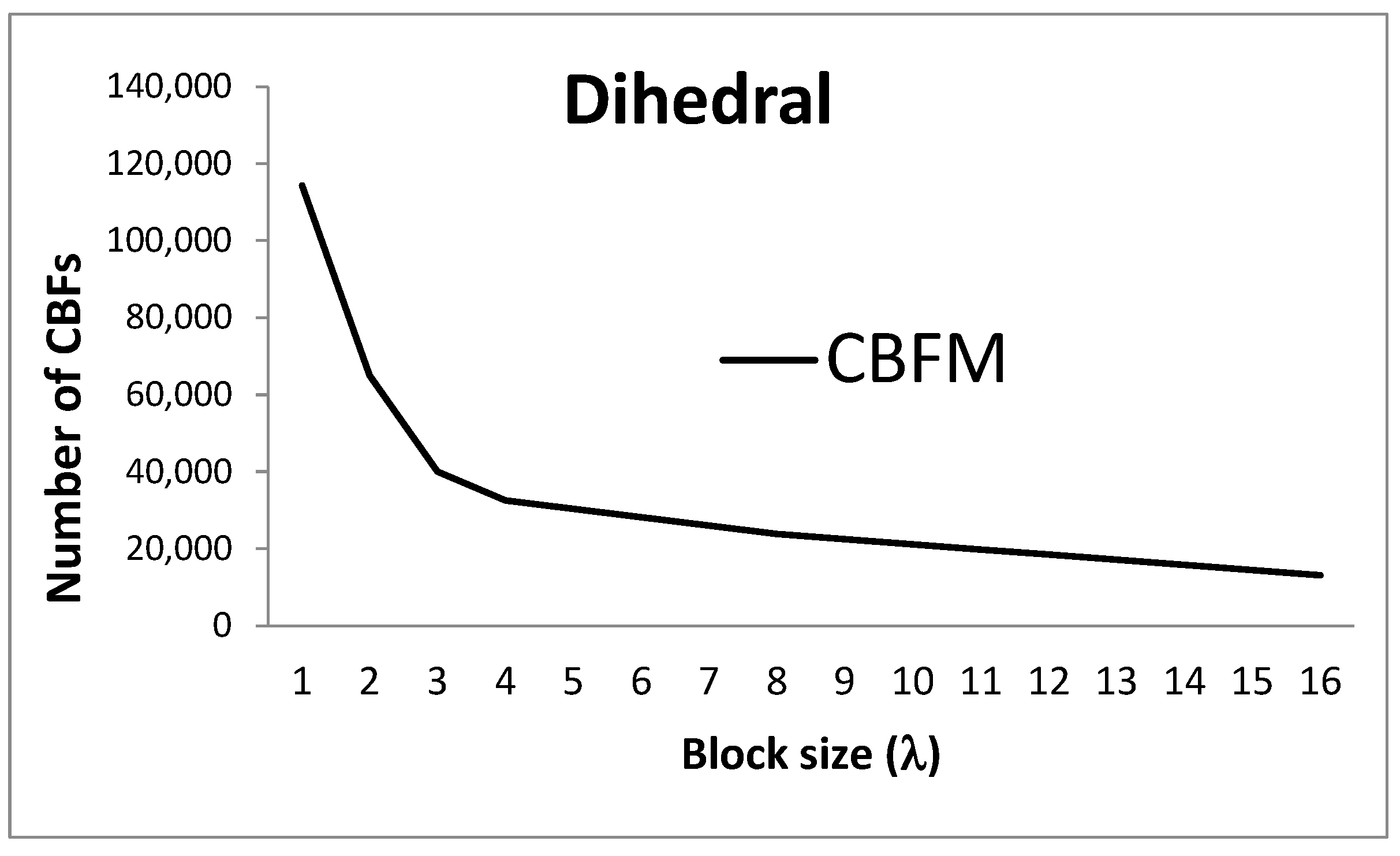
The CBFs are defined over blocks, which generally present a cubic shape with a typical side length of one or two wavelengths. The CBFs need to be calculated in a pre-processing stage. The number of low-level basis functions is higher than the total number of CBFs on each block, which results in a faster system solution. The size of the blocks has a direct impact on the reduction in the number of unknowns, and, in order to illustrate this effect, Figure 1 shows the number of CBFs computed for different block sizes considering a 90° dihedral, where each plate has a side length of 32 wavelengths. The block size ranges from 1 to 16 wavelengths. The total number of low-level basis functions in this case is 413,770.

Note that Figure 1 presents the total number of unknowns in the problem using different block sizes. The total number of low-level basis functions would not change with the block size. The ratio between the number of CBFs and the number of low-level functions is about 3.8 for blocks with a size of λ and 31.5 for blocks with a size of 16λ.

Considering the results shown in Figure 1, it appears to be desirable to make use of large blocks in order to reduce the effective size of the problem. However, we need to consider that large blocks can involve a drastic increase in the CPU time required in some stages of the conventional CBF generation process.

The CBFM can be considered a modification of the conventional MoM with some additional steps to account for the inclusion of the new basis functions. It is noteworthy to point out that the CBFM is especially beneficial in those cases where the reduction in the CPU time for the system solution exceeds the processing time invested in the generation of the CBFs and their coupling matrix, as is generally the case for the analysis of problems involving multiple excitations and/or frequencies. Furthermore, the CBFM can be well suited for moderately sized, ill-conditioned problems that are amenable to a direct solution given the reduction in the number of unknowns obtained after the definition of the new set of basis functions.

With the previous considerations, the CBFM can be considered advantageous to the extent that its preprocessing time can be minimized for relatively large blocks. Some previous works have dealt with merging already computed CBFs into new sets over combined blocks [23] or other techniques focused on the fast computation of the CBFs using angular subranges [25]. The combination of the CBFM and the MLFMM shown in [26] allows for the fast computation of the reduced matrix by avoiding the need to store impedance terms between CBFs that are not defined on the same or adjacent blocks.

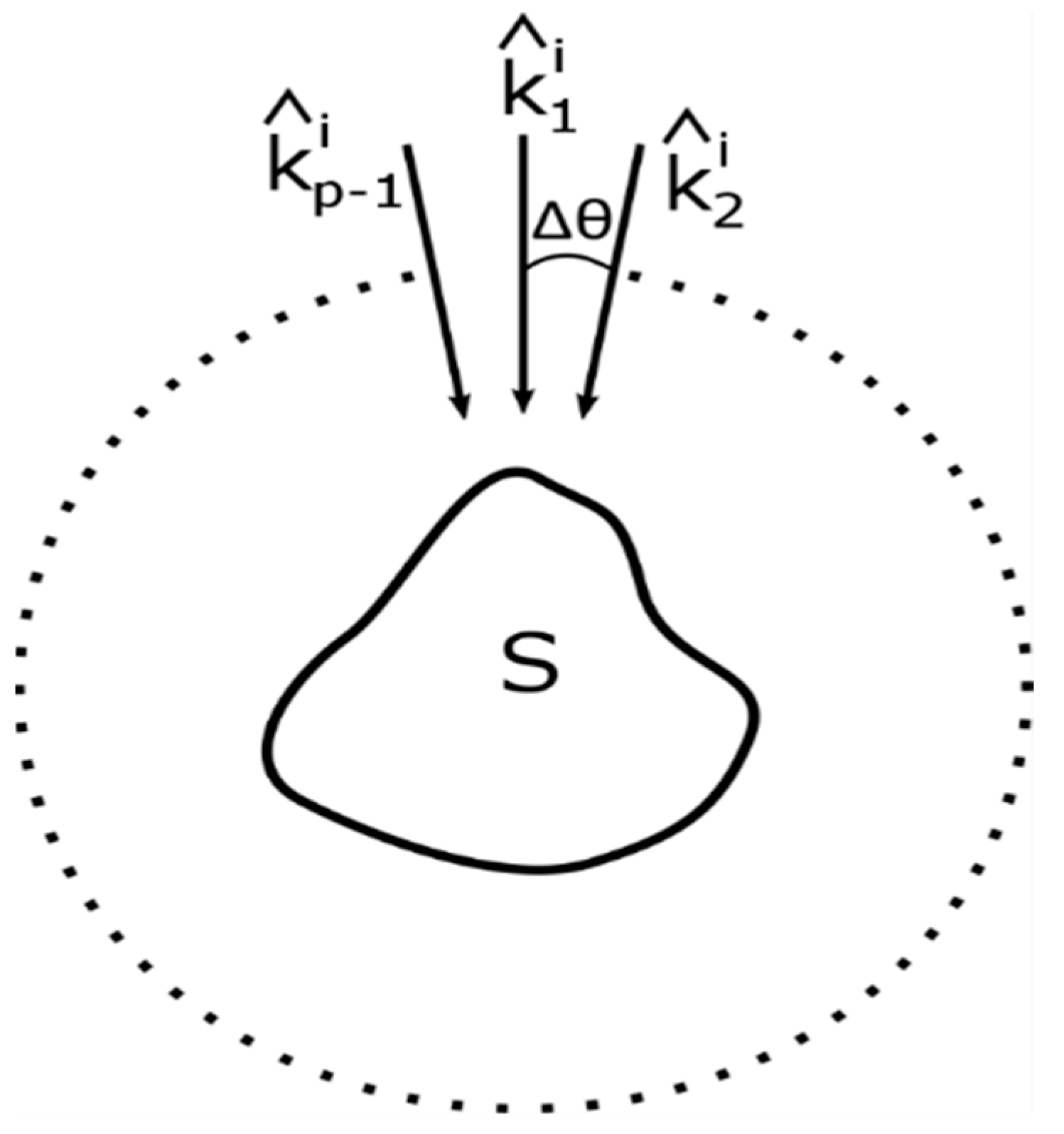
It is relatively common to generate CBFs by means of the singular value decomposition (SVD) of a set of currents induced by sampling the Plane Wave Spectrum (PWS) impinging over each isolated block [21]. Figure 2 illustrates this situation, where the angular step or separation between plane waves (Δθ) depends on the block size [27].

The SVD provides a new orthogonal base that can be truncated by applying a threshold to the corresponding singular values. This truncation provides the reduction in the number of unknowns. Note, in addition, that the computation of the currents induced by the PWS can be carried out using PO, which considers that the current value on a given low-level basis function depends only on the impressed voltage, or MoM, where all the low-level basis functions belonging to the block are coupled. PO-based CBFs can evidently be computed faster and provide accurate results as long as the surfaces contained on the block are relatively smooth and free of discontinuities or small details. MoM-based CBFs do not have restrictions regarding the geometrical features of the block, but they require additional processing time. After the CBFs have been obtained following this procedure, they can effectively model the current distribution induced by different real sources in the scenario and be stored and re-used for other analyses as long as the mesh does not change.

The reduced matrix contains the coupling terms between CBFs located on the same or different blocks. In order to build this matrix, it is possible to make use of the conventional low-level MoM impedance coefficients and aggregate them using the already computed CBF weight values. A generic coefficient, Z_m,n, containing the coupling value between source CBF-n (identified as J_j,n) located on block j and the testing source CBF-m (identified as ${\mathrm{W}}_{\mathrm{m}}^{\mathrm{i}}$) located on block i can be written as shown in (1):

$${\mathrm{Z}}_{\mathrm{m},\mathrm{n}}=⟨\mathrm{L}({\mathrm{J}}_{\mathrm{j},\mathrm{n}}),{\mathrm{W}}_{\mathrm{m}}^{\mathrm{i}}⟩={\sum }_{\mathrm{k}=1}^{{\mathrm{N}}_{\mathrm{i}}}{\sum }_{\mathrm{l}=1}^{{\mathrm{N}}_{\mathrm{j}}}{\mathsf{\alpha }}_{\mathrm{j},\mathrm{n}}(\mathrm{l}){\mathsf{\alpha }}_{\mathrm{i},\mathrm{m}}^{\mathrm{*}}(\mathrm{k})⟨{\mathrm{T}}_{\mathrm{l}}(\mathrm{u},\mathrm{v}),{\mathrm{R}}_{\mathrm{k}}({\mathrm{u}}^{\prime },{\mathrm{v}}^{\prime })⟩$$

(1)

where $⟨\mathrm{L}({\mathrm{J}}_{\mathrm{j},\mathrm{n}}),{\mathrm{W}}_{\mathrm{m}}^{\mathrm{i}}⟩$ is the inner product, ${\mathrm{T}}_{\mathrm{l}}(\mathrm{u},\mathrm{v})$ and ${\mathrm{R}}_{\mathrm{k}}(\mathrm{u}\prime ,\mathrm{v}\prime )$ are the l-th and k-th low-level basis and testing functions on blocks j and i, respectively, and ${\mathsf{\alpha }}_{\mathrm{j},\mathrm{n}}(\mathrm{l})$ represents the weight of the l-th low-level basis function on block j for CBF-n. Each CBF requires, therefore, the storage of a linear combination of weights of the low-level basis functions on the corresponding block:

$${\mathrm{J}}_{\mathrm{i},\mathrm{k}}(\mathrm{u},\mathrm{v})={\sum }_{\mathrm{n}=1}^{{\mathrm{N}}_{\mathrm{i}}}{\mathsf{\alpha }}_{\mathrm{i},\mathrm{k}}(\mathrm{n}){\mathrm{T}}_{\mathrm{n}}(\mathrm{u},\mathrm{v})$$

(2)

$${\mathrm{W}}_{\mathrm{k}}^{\mathrm{i}}(\mathrm{u},\mathrm{v})={\sum }_{\mathrm{n}=1}^{{\mathrm{N}}_{\mathrm{i}}}{\mathsf{\alpha }}_{\mathrm{i},\mathrm{k}}(\mathrm{n}){\mathrm{R}}_{\mathrm{n}}(\mathrm{u},\mathrm{v})$$

(3)

and, with these considerations, it is possible to substitute the inner product in (1) with the corresponding low-level impedance coefficient, z_k,l:

$${\mathrm{Z}}_{\mathrm{m},\mathrm{n}}={\sum }_{\mathrm{k}=1}^{{\mathrm{N}}_{\mathrm{i}}}{\sum }_{\mathrm{l}=1}^{{\mathrm{N}}_{\mathrm{j}}}{\mathsf{\alpha }}_{\mathrm{j},\mathrm{n}}(\mathrm{l}){\mathsf{\alpha }}_{\mathrm{i},\mathrm{m}}^{\mathrm{*}}(\mathrm{k}){\mathrm{z}}_{\mathrm{k},\mathrm{l}}$$

(4)

Note that in the previous expression, we made use of uppercase to make reference to CBF impedance coefficients and lowercase for low-level impedance coefficients, respectively.

An important alternative to the computation of the full reduced matrix using (4) involves the use of the MLFMM to consider the far-field interactions between the low-level basis functions. In this case, the introduction of the MLFMM combined with the CBFM splits the computation of Z_m,n in (4) into two different terms:

$${\mathrm{Z}}_{\mathrm{m},\mathrm{n}}={\mathrm{Z}}_{\mathrm{m},\mathrm{n}}^{\mathrm{n}\mathrm{f}}+{\mathrm{Z}}_{\mathrm{m},\mathrm{n}}^{\mathrm{f}\mathrm{f}}$$

(5)

where ${\mathrm{Z}}_{\mathrm{m},\mathrm{n}}^{\mathrm{n}\mathrm{f}}$ and ${\mathrm{Z}}_{\mathrm{m},\mathrm{n}}^{\mathrm{f}\mathrm{f}}$ contain, respectively, the near- and far-field contributions from the low-level basis functions. The ${\mathrm{Z}}_{\mathrm{m},\mathrm{n}}^{\mathrm{n}\mathrm{f}}$ term is then calculated as a modification of (4), where we only consider the contribution of ${\mathrm{N}}_{\mathrm{m}}^{\mathrm{n}\mathrm{f}}·{\mathrm{N}}_{\mathrm{n}}^{\mathrm{n}\mathrm{f}}$ near-field impedance coefficients:

$${\mathrm{Z}}_{\mathrm{m},\mathrm{n}}^{\mathrm{n}\mathrm{f}}={\sum }_{\mathrm{k}=1}^{{\mathrm{N}}_{\mathrm{i}}^{\mathrm{n}\mathrm{f}}}{\sum }_{\mathrm{l}=1}^{{\mathrm{N}}_{\mathrm{j}}^{\mathrm{n}\mathrm{f}}}{\mathsf{\alpha }}_{\mathrm{j},\mathrm{n}}(\mathrm{l}){\mathsf{\alpha }}_{\mathrm{i},\mathrm{m}}^{\mathrm{*}}(\mathrm{k}){\mathrm{z}}_{\mathrm{k},\mathrm{l}}.$$

(6)

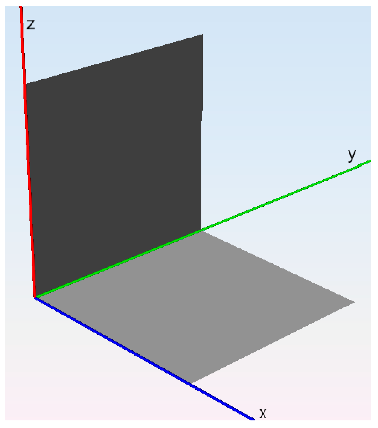
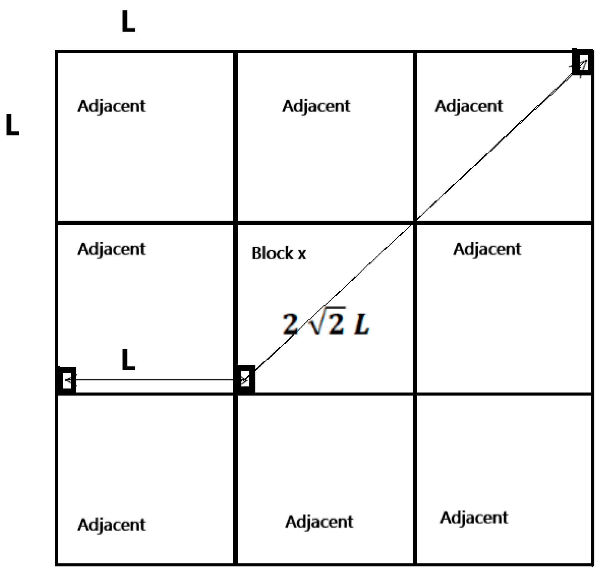
In order to achieve this, it is possible to, after having obtained the geometric partitioning in terms of blocks, divide the blocks recursively into regions until reaching a first region level of around 0.25λ. In this case, only the low-level impedance terms within each block and its neighbors need to be computed and stored, and their contribution to the computation of the reduced matrix coefficients can be accounted for using (6). In a 2D scenario, the near-field coupling distance can range from 0 to $2\sqrt{2}\mathrm{L},$ where L is the region size, with a typical value of 0.25λ, as seen in Figure 3.

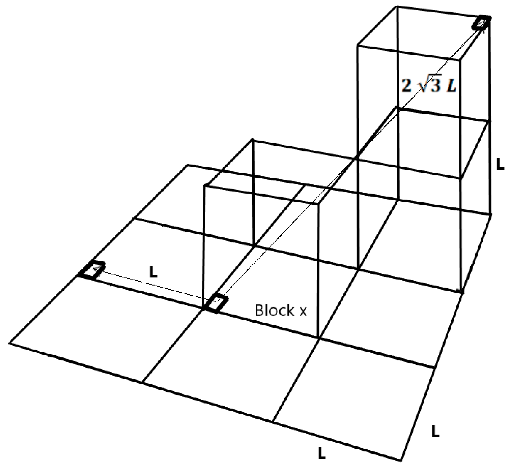
In the case of 3D geometries, the distance between the elements contained in the sparse near-field impedance matrix ranges from 0 to $2\sqrt{3}\mathrm{L},$ assuming, for the sake of simplicity, that each region is a perfect cube (Figure 4).

The rest of the interactions can be considered by the aggregation, translation and disaggregation of the low-level functions:

$${\mathrm{z}}_{\mathrm{i},\mathrm{j}}^{\mathrm{f}\mathrm{f}}=\int {\mathrm{V}}_{\mathrm{m}\mathrm{j}}^{\mathrm{A}\mathrm{G}\mathrm{G}}(\widehat{\mathrm{k}}){\mathsf{\tau }}_{\mathrm{m}\mathrm{m}\prime }(\widehat{\mathrm{k}},{\overrightarrow{\mathrm{r}}}_{\mathrm{m}\mathrm{m}\prime }).{\mathrm{V}}_{\mathrm{m}\prime \mathrm{i}}^{\mathrm{D}\mathrm{I}\mathrm{S}}(\widehat{\mathrm{k}}){\mathrm{d}}^2\widehat{\mathrm{k}}$$

(7)

where ${\mathrm{V}}_{\mathrm{m}\mathrm{j}}^{\mathrm{A}\mathrm{G}\mathrm{G}}(\widehat{\mathrm{k}})$ is the aggregation term of low-level basis function j to the center of region m and is computed as follows:

$${\mathrm{V}}_{\mathrm{m}\mathrm{j}}^{\mathrm{A}\mathrm{G}\mathrm{G}}(\widehat{\mathrm{k}})={\int }_{\mathrm{u}}{\int }_{\mathrm{v}}{\mathrm{e}}^{-\mathrm{j}\widehat{\mathrm{k}}\cdot \overrightarrow{{\mathrm{r}}_{\mathrm{j}\mathrm{m}}}}\left(\overline{\mathrm{I}}-\widehat{\mathrm{k}}\widehat{\mathrm{k}}\right)·\overrightarrow{{\mathrm{T}}_{\mathrm{j}}}(\mathrm{u},\mathrm{v})\mathrm{d}\mathrm{u}\mathrm{d}\mathrm{v}$$

(8)

where ${\overrightarrow{\mathrm{r}}}_{\mathrm{j},\mathrm{m}}$ is the position vector from each integration point to the center of cube m and ${\mathrm{T}}_{\mathrm{j}}(\mathrm{u},\mathrm{v})$ is the basis function considered.

The expression for the computation of the disaggregation term is as follows:

$${\mathrm{V}}_{\mathrm{m}\prime \mathrm{i}}^{\mathrm{D}\mathrm{I}\mathrm{S}}(\widehat{\mathrm{k}})={\int }_{\mathrm{u}}{\int }_{\mathrm{v}}{\mathrm{e}}^{\mathrm{j}\widehat{\mathrm{k}}\cdot \overrightarrow{{\mathrm{r}}_{\mathrm{i}\mathrm{m}\prime }}}\left(\overline{\mathrm{I}}-\widehat{\mathrm{k}}\widehat{\mathrm{k}}\right)·\overrightarrow{{\mathrm{R}}_{\mathrm{i}}}(\mathrm{u},\mathrm{v})\mathrm{d}\mathrm{u}\mathrm{d}\mathrm{v}$$

(9)

where ${\mathrm{R}}_{\mathrm{i}}(\mathrm{u},\mathrm{v})$ is the testing function. Finally, the translation term, ${\mathsf{\tau }}_{\mathrm{m}\mathrm{m}\prime }$ between points m and m′ can be computed as follows:

$${\mathsf{\tau }}_{\mathrm{m}\mathrm{m}\prime }(\widehat{\mathrm{k}},{\overrightarrow{\mathrm{r}}}_{\mathrm{m}\mathrm{m}\prime })=\frac{\mathrm{j}\mathrm{k}}{4\mathsf{\pi }}{\sum }_{\mathrm{l}=0}^{\mathrm{L}}{\mathrm{j}}^{\mathrm{l}}(2\mathrm{l}+1){\mathrm{h}}_{\mathrm{l}}^{(1)}(\mathrm{k}{\mathrm{r}}_{\mathrm{m}\mathrm{m}\prime }){\mathrm{P}}_{\mathrm{l}}({\widehat{\mathrm{r}}}_{\mathrm{m}\mathrm{m}\prime }\cdot \widehat{\mathrm{k}})$$

(10)

where ${\mathrm{h}}_{\mathrm{l}}^{(1)}(\mathrm{k}{\mathrm{r}}_{\mathrm{m}\mathrm{m}\prime })$ is a spherical Hankel function of the first kind and ${\mathrm{P}}_{\mathrm{l}}({\widehat{\mathrm{r}}}_{{\mathrm{m}\mathrm{m}}^{\prime }}\widehat{\mathrm{k}})$ is a Legendre polynomial. The integral in (5) is defined over k-space on a Ewald sphere but can be truncated to a number of points that provide a non-significant error [2].

With the previous considerations, the computation of the far-field coupling contributions to the Z_m,n coefficient of the reduced matrix is expressed as follows:

$$\begin{array}{c}{\mathrm{Z}}_{\mathrm{m},\mathrm{n}}^{\mathrm{f}\mathrm{f}}={\displaystyle \sum _{\mathrm{k}=1}^{{\mathrm{N}}_{\mathrm{i}}^{\mathrm{f}\mathrm{f}}}}{\displaystyle \sum _{\mathrm{l}=1}^{{\mathrm{N}}_{\mathrm{j}}^{\mathrm{f}\mathrm{f}}}}{\mathsf{\alpha }}_{\mathrm{j},\mathrm{n}}(\mathrm{l}){\mathsf{\alpha }}_{\mathrm{i},\mathrm{m}}^{\mathrm{*}}(\mathrm{k})\int {\mathrm{V}}_{\mathrm{p}\mathrm{j}}^{\mathrm{A}\mathrm{G}\mathrm{G}}(\widehat{\mathrm{k}}){\mathsf{\tau }}_{\mathrm{p}\mathrm{p}\prime }(\widehat{\mathrm{k}},{\overrightarrow{\mathrm{r}}}_{\mathrm{p}\mathrm{p}\prime }).{\mathrm{V}}_{\mathrm{p}\prime \mathrm{i}}^{\mathrm{D}\mathrm{I}\mathrm{S}}(\widehat{\mathrm{k}}){\mathrm{d}}^2\widehat{\mathrm{k}}\\ \hspace{1em}\hspace{1em}\hspace{1em}\hspace{1em}\hspace{1em}\hspace{1em}\hspace{1em}\hspace{1em}\hspace{1em}\hspace{1em}=\int {\mathrm{d}}^2\widehat{\mathrm{k}}{\displaystyle \sum _{\mathrm{l}=1}^{{\mathrm{N}}_{\mathrm{j}}^{\mathrm{f}\mathrm{f}}}}{\mathsf{\alpha }}_{\mathrm{j},\mathrm{n}}(\mathrm{l}){\mathrm{V}}_{\mathrm{p}\mathrm{j}}^{\mathrm{A}\mathrm{G}\mathrm{G}}(\widehat{\mathrm{k}}){\mathsf{\tau }}_{\mathrm{p}\mathrm{p}\prime }(\widehat{\mathrm{k}},{\overrightarrow{\mathrm{r}}}_{\mathrm{p}\mathrm{p}\prime }){\displaystyle \sum _{\mathrm{k}=1}^{{\mathrm{N}}_{\mathrm{i}}^{\mathrm{f}\mathrm{f}}}}{\mathsf{\alpha }}_{\mathrm{i},\mathrm{p}}^{\mathrm{*}}(\mathrm{k}){\mathrm{V}}_{\mathrm{p}\prime \mathrm{i}}^{\mathrm{D}\mathrm{I}\mathrm{S}}(\widehat{\mathrm{k}})\end{array}$$

(11)

where p refers to the center of the region in which the l-th low-level basis function of block n is contained and p′ indicates the center of the region containing the k-th low-level testing function in block m.

3. Definition of the Proposed Approach

The work presented here aims to reduce the CPU time required by the most computationally expensive stages of the CBFM, the generation of the CBFs and the reduced matrix, without compromising the accuracy. This efficiency improvement helps reduce the inherent burden of the CBFM when processing large blocks, allowing for a more pronounced reduction in the number of unknowns, as discussed in the previous section.

It has been previously mentioned that asymptotic approaches can be used to obtain CBFs, although their use is constrained by the specific details contained in the block. MoM-based CBFs, on the other hand, include interactions between different parts of the block when generating the CBFs, which makes the CBFM pre-processing time increase when making use of large block sizes.

A new approach for the efficient generation of CBFs is presented in this section, in which the generation of the CBFs takes into account exclusively the near-field low-level impedance matrix of each block. This matrix is later used for the generation of the reduced matrix, and consequently, it can be re-used for that stage without involving any additional computational cost. We have considered that it is necessary to make use of an approach that allows a dynamic selection of the number of coupling terms to be considered, or, in other words, that defines a near-field criterion. This can be especially important if this approach is going to be applied to analyses using blocks of different sizes or if some blocks in the scenario present geometric features that require a higher degree of accuracy when representing the induced currents. Note that, although only the near-field part of the coupling matrix is used for the CBF generation, the use of the MLFMM takes into account far-field coupling terms in the computation of the reduced matrix and in the solution of the global system.

Taking the previous ideas into account, we propose in this work the introduction of a normalized distance parameter, Ψ, that defines which near-field coupling terms will be considered for the creation of CBFs, discarding those that correspond to interactions between more distant low-level basis and testing functions. This parameter will have a defined range between 0 and 1. The value 0 indicates that the current is produced solely by the incident field where the given basis function is defined. On the other hand, all the coupling terms corresponding to basis functions inside the block will be considered if the distance parameter, Ψ, is set to 1. This process is described in detail in [28], where an absolute distance parameter is used to discriminate between the near-field coupling terms to be considered.

When computing the CBFs using MoM-based currents, it is necessary to consider an extension of the block in order to avoid artificially introduced edge effects [18]. This is achieved by adding coupling terms belonging to neighboring basis functions that can belong to other blocks and discarding these currents after they are obtained. The Ψ parameter therefore needs to be increased by a distance that allows the edge effect to be avoided, which in our experience is typically around 0.25 wavelengths.

The application of the Ψ threshold parameter when computing the CBFs produces a sparse near-field coupling matrix that can be seen as an approximate version of the rigorous coupling matrix associated with the block. The CBFs are then obtained using this matrix to compute the currents induced by the PWS on the block and applying SVD for their orthonormalization. One advantage of the proposed technique is that it avoids the restrictions imposed by the use of PO-based CBFs and can be used regardless of the complexity of the geometry inside each block. At the same time, the generation of the CBFs is much faster than when using the conventional MoM-based technique. It also allows the computational cost of this stage to be adjusted depending on the characteristics of each block. The sparse coupling matrix produced benefits from, in addition to the reduced memory footprint, the use of specific algorithms and libraries that address the efficient solution of systems defined by sparse matrices. Note that these advantages increase with the block size.

An additional modification that serves to accelerate the generation of MoM-based CBFs can be introduced by making use of a pseudoinverse matrix computed as a sparse approximate inverse (SAI) operator. It is common to use near-field SAI matrices as preconditioners [29], although our proposal is to apply them to compute an approximation of the induced current distribution on each block given a certain excitation:

$${\mathrm{J}}^{(\mathrm{i})}\cong \left[\mathrm{M}\right]·{\mathrm{V}}^{(\mathrm{i})}$$

(12)

where i is the index of the considered excitation surrounding the block, ${\mathrm{J}}^{(\mathrm{i})}$ represents the approximated solution of the current and ${\mathrm{V}}^{(\mathrm{i})}$ stands for the i-th impressed voltage. In turn, [M] is the SAI matrix obtained using the near-field sparsity pattern [30]. The potential lack of accuracy of these currents is compensated by the diversity of excitations considered. Note that for a block size of over 2λ, it can be necessary to obtain the currents induced by over 10,000 plane waves, which can be performed extremely quickly by making use of (12). We integrated the definition of the Ψ parameter into the sparsity pattern of the approximate sparse inverse matrix as follows: when $\mathsf{\Psi }\le 0.5,$ the sparsity pattern of [M] matches exactly that of the near-field low-level coupling matrix. However, for $\mathsf{\Psi }>0.5,$ the size of the approximate inverse matrix may make the computation inefficient, and in that case, the sparsity pattern of [M] used is the same as the near-field pattern associated with the first-level MLFMM boxes.

It should be highlighted that determining the appropriate value for the Ψ parameter is important for a correct balance between efficiency and accuracy. This value is influenced by the complexity of each block, so aspects such as the number of distinct objects to which the geometric elements of the block belong, the curvature of these objects, the mesh density used to define the low-level base functions and the material they are composed of should be taken into account. Moreover, it is common to find realistic problems that present smooth regions combined with more complex parts. An example of this type of scenario is the analysis of an airplane, with smooth surfaces modeling a significant portion of the geometry (such as the fuselage), but these are combined with other parts such as inlets or other cavities with very small details. This scenario is often referred to as a multiscale problem. The proposed technique proves useful in addressing such problems, as it allows for the definition of a different parameter value for each block. Values close to 0.0 can be used in smooth regions, while values close to 1.0 can be applied to more complex areas.

For large simulations running on computing clusters, no additional considerations need to be taken into account regarding the block size of the Ψ parameter value. However, in order to favor load-balancing features with the MLFMM, it could be necessary to establish a maximum aggregation level or to combine the distribution of boxes with the distribution of angular directions in order to reduce communication between computing nodes.

4. Results

This section contains a number of test cases selected in order to show the accuracy and efficiency of the approach described in the previous section.

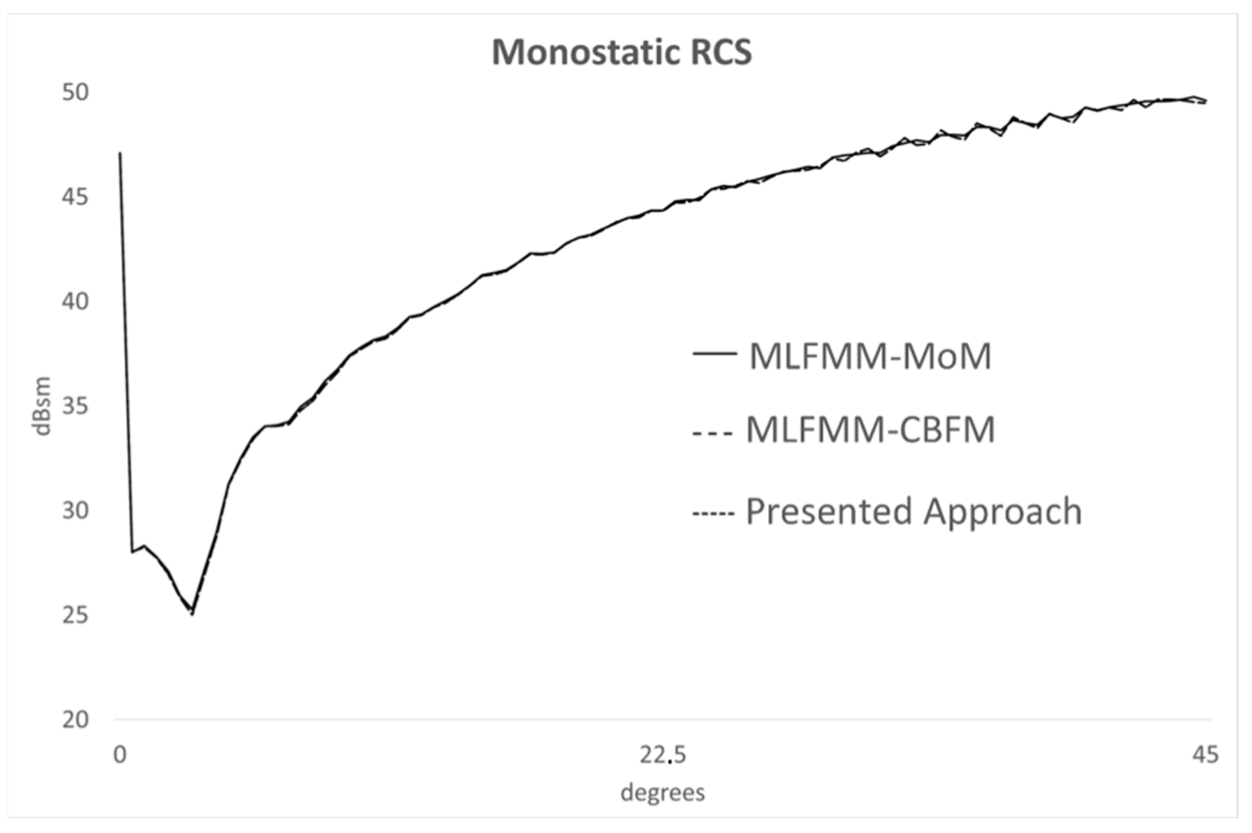
The first test case covers the monostatic RCS computation of a 64λ dihedral angle, shown in Figure 5, considering an angular observation cut at φ = 0°, with θ ranging from 0° to 45° in 0.5° steps. The total number of low-level unknowns is 1,657,012. Figure 6 compares the results obtained using the MLFMM–MoM technique, the conventional MLFMM–CBFM technique and the proposed accelerated MLFMM–CBFM technique, which we have identified as CBFMnf. The problem was analyzed using block sizes of 2λ and 4λ, and the Ψ parameter was 0.125. Good agreement can be observed between the three solutions provided. The restarted Biconjugate Gradient Stabilized method (BiCGStab) [31] was used to solve the complete system in all the examples provided.

Considering that this work addresses the efficiency improvement of existing approaches, a comparison of the processing time and memory usage for the computation of the CBFs of one block is also provided in

Table 1. CPU time spent for the computation of the CBFs in a block with a size of 2λ.

	Conventional System Resolution	Sparse Near-Field Resolution	SPAI
CPU time	342 s	297 s	98 s
Memory requirements	584 Mb	123 Mb	109 Mb

.

Finally,

Table 2. CPU time spent for the computation of the CBFs in a block with a size of 4λ.

	MLFMM–MoM	MLFMM–CBFM (MoM-Based CBFs)	MLFMM–CBFMnf
Number of unknowns	1,657,012	470,390	468,258
Creation of CBFs	-	23,456 s	11,346 s
Coupling Matrix	1183 s	2109 s	1403 s
Total CPU time	190,039 s	102,146 s	62,803 s

shows a comparison of the CPU time required by the main stages of the simulation (creation of the CBFs, computation of the reduced matrix and system solution) using the MLFMM–MoM approach, the MLFMM–CBFM technique and the proposed approach. In this case, the proposed approach (CBFMnf) made use of the SAI matrix for the fast computation of the CBFs.

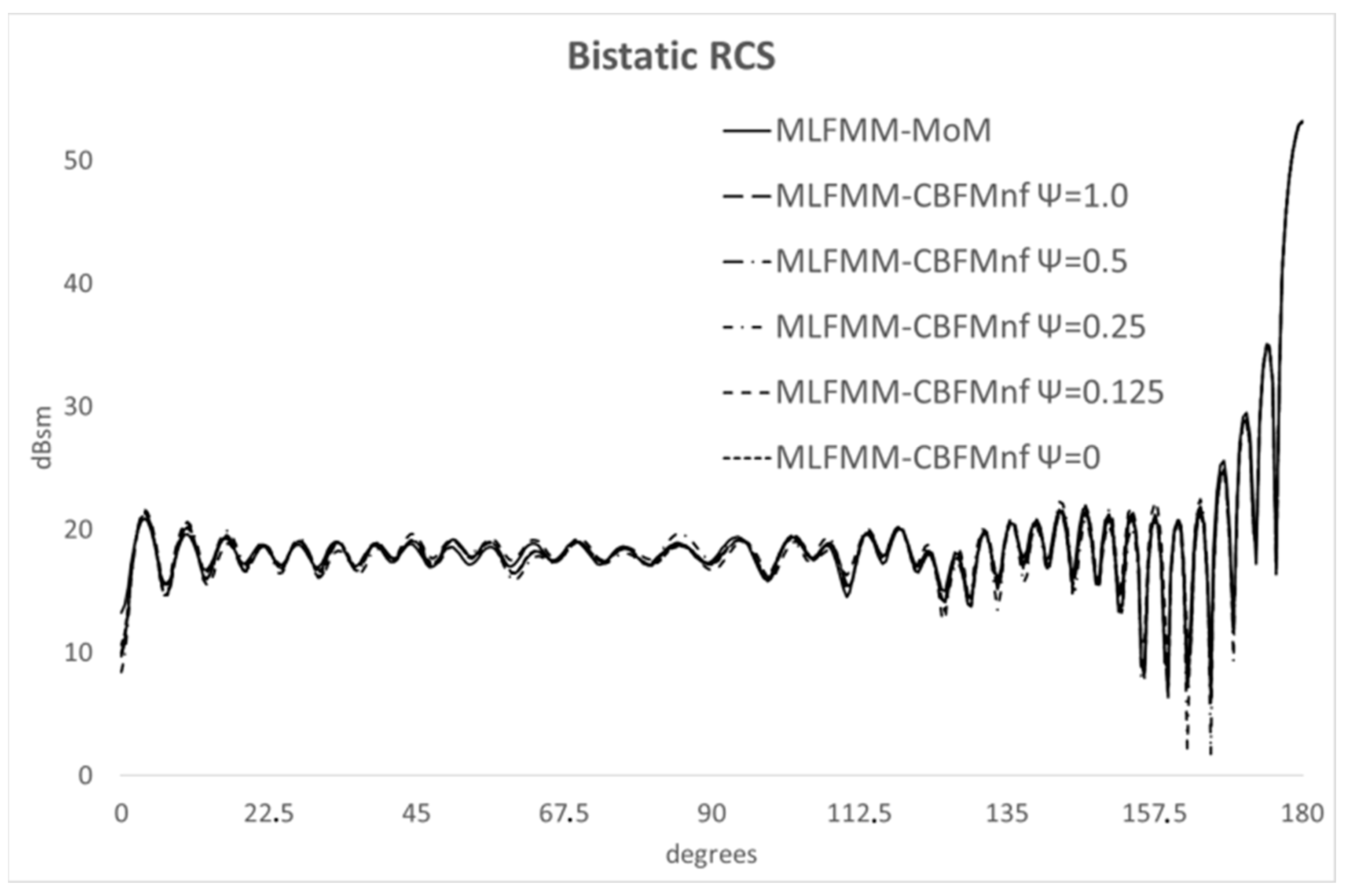
The next test case deals with the computation of the bistatic RCS of a hemisphere with a radius of 9λ, oriented with the normal vector of its pole along $\widehat{\mathrm{z}}$. The structure is illuminated from θ = 0° and ϕ = 0°, and the observation directions are in the ϕ = 0° plane, ranging from θ = 0° to θ = 180°. The size of the blocks used to analyze this structure was 2λ. This case was analyzed using several Ψ parameter values ranging from 0.0 to 1.0. For this geometry, there is good agreement between the results obtained using the MLFMM–MoM technique and the proposed approach using different Ψ thresholds, as shown in Figure 7.

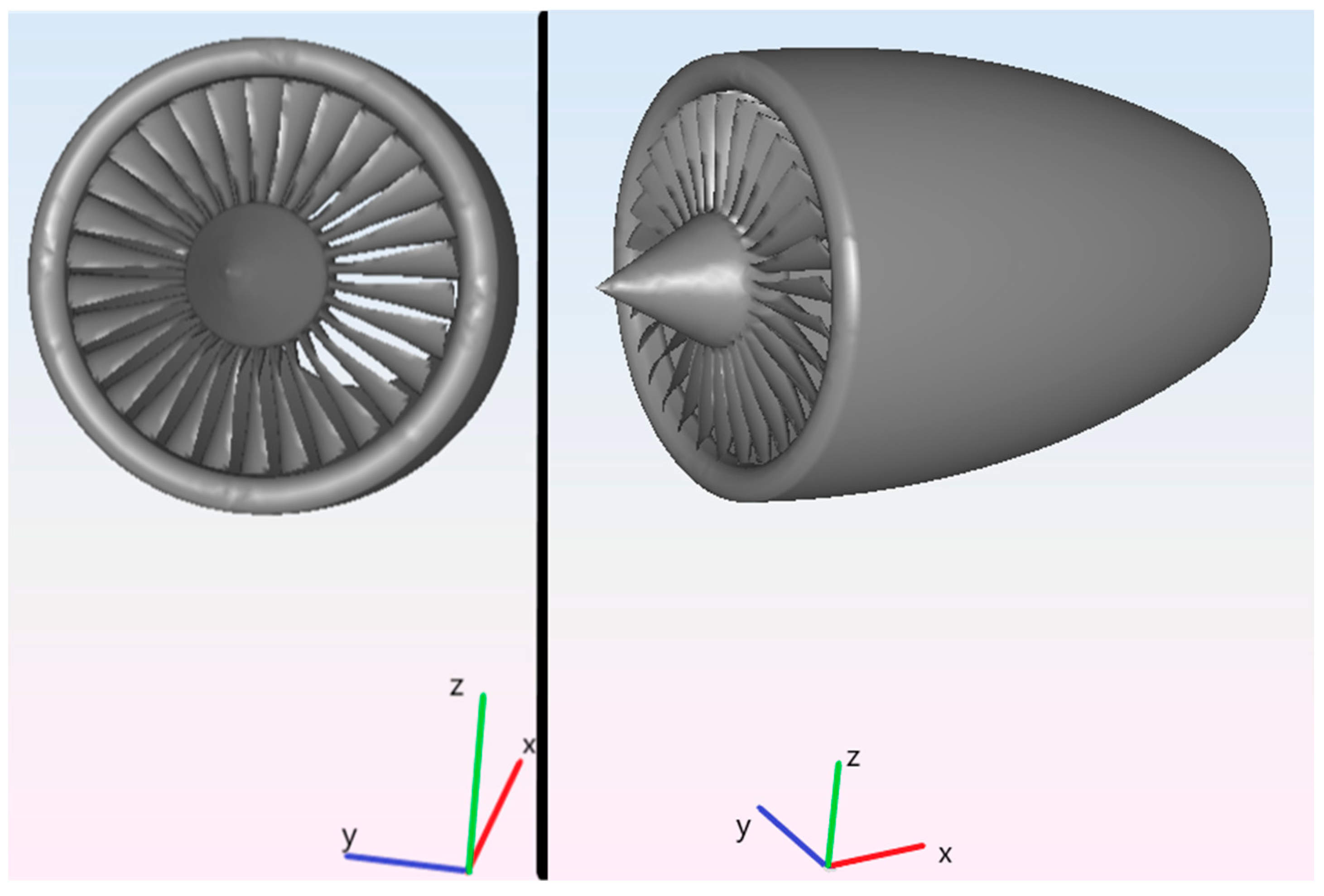
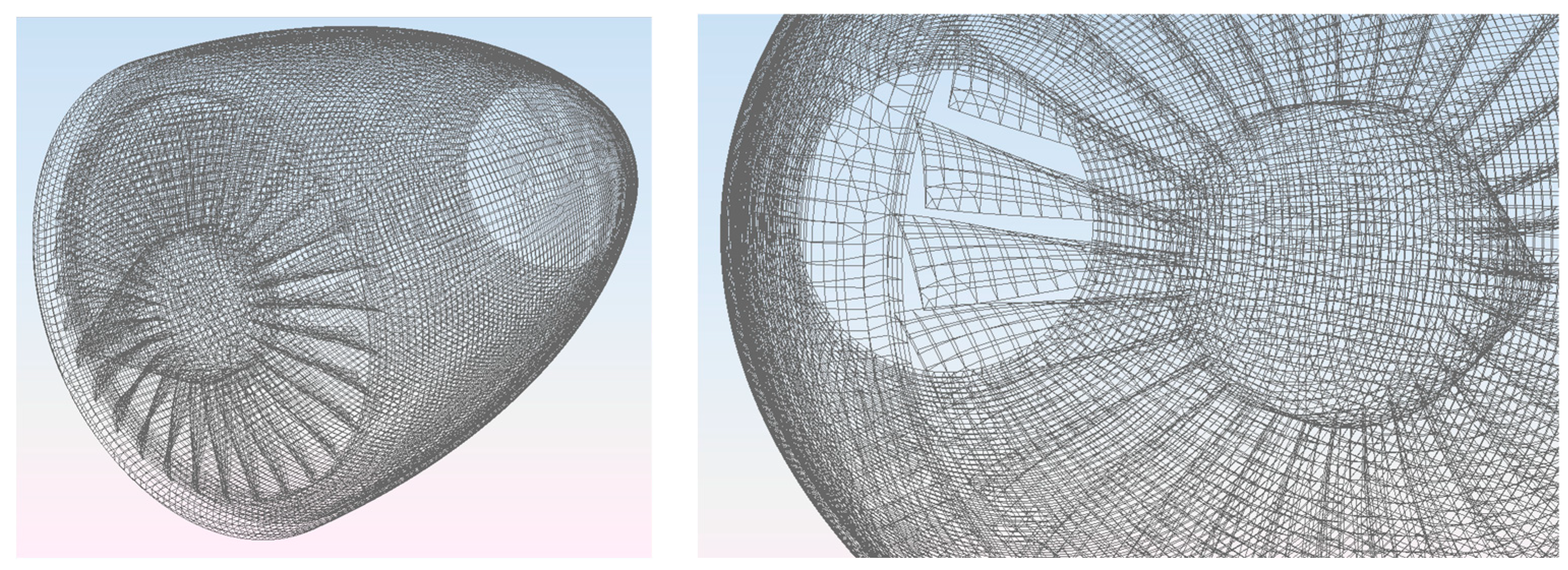
The last test case is the analysis of the aircraft engine depicted in Figure 8, for which the monostatic RCS was obtained at a frequency of 4 GHz. The length of this structure is 730 mm, and its maximum diameter is 405 mm. The incident plane for this analysis is θ = 90°, covering 361 directions from ϕ = 90° to 270° in 0.5° steps. The total number of unknowns was 66,237 when applying the MLFMM–MoM technique, and that number was reduced to 2327 and 2542 unknowns when using the MLFMM–CBFM technique (MoM-based CBFs) and the proposed approach, respectively.

Considering the complexity of this geometry, Figure 9 provides some additional details of the resulting mesh. It can be seen that there are triangular and quadrangular elements combined. These elements are described as Bezier patches, described by 3 × 3 control points, which, in some cases, can be degenerate, resulting in a triangular shape. The low-level basis functions used are curved rooftops, and the testing functions are curved razor blades. The use of mesh elements that are conformal to the original geometry allows for a reduction in the facetization errors for a given sampling density or a relaxation of the mesh density while maintaining a certain degree of accuracy. The total number of mesh elements obtained was 33,362 in this case. There are 30 blades, where each blade has a thickness of 3 mm and a length of 100 mm.

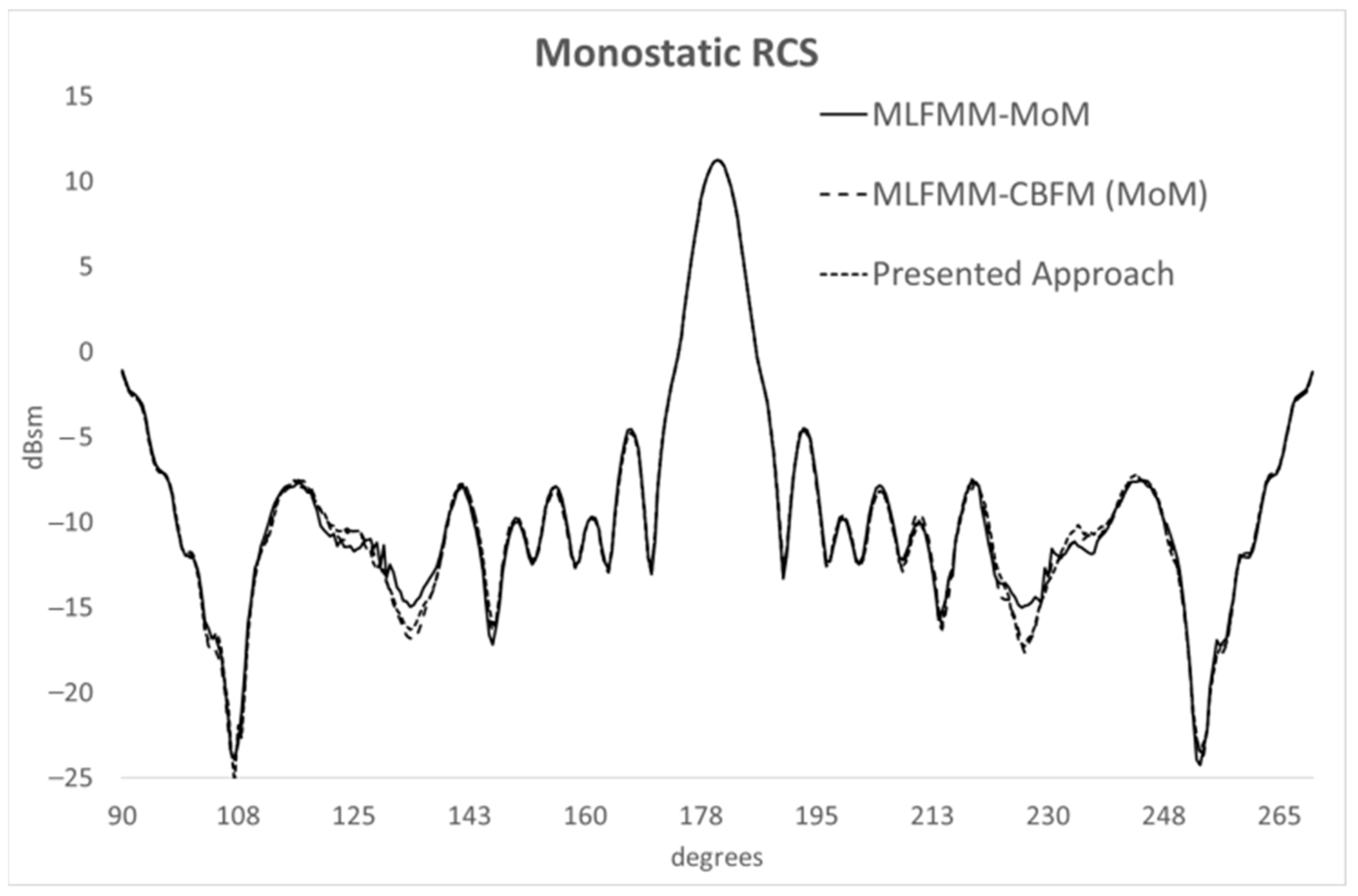
The results obtained are shown in Figure 10, where we can observe good agreement between the three different techniques: (i) the MLFMM–MoM technique, taken as the reference given that it is a mature solver and has been extensively validated, (ii) the MLFMM–CBFM technique, using MoM-based CBFs computed by the conventional procedure and (iii) the proposed approach, where we set Ψ = 0.0 for the external surfaces of the engine, Ψ = 0.5 for the central cone oriented along the x axis and Ψ = 1.0 for the blades of the turbine. The CPU time when applying the MLFMM–MoM technique, the MLFMM–CBFM technique (MoM-based CBFs) and the proposed technique (MLFMM-CBFMnf) is outlined in

Table 3. CPU time results related to the analysis of the engine.

	MLFMM–MoM	MLFMM–CBFM (MoM-Based CBFs)	MLFMM–CBFMnf
Number of unknowns	66,237	2327	2542
Preprocessing	-	4137 s	1338 s
Total CPU time	40,266 s	23,423 s	21,042 s

. The average number of iterations required by the proposed approach was about 2% higher than that required for the MLFMM–CBFM (MoM) technique, which is justified since the new CBF computation method makes approximations that can result in slightly less accurate current distributions, but at the same time, this can be considered to introduce a negligible impact on the overall convergence.

5. Conclusions

A novel approach for the computation of Characteristic Basis Functions was developed in this work, focusing on the efficiency improvements obtained when considering large blocks. A parametrized algorithm for the selection of the near-field coupling terms of the impedance matrix for each block is used, allowing us to assign different thresholds to blocks with special features. A pseudoinverse matrix is also used to accelerate the computation of the approximated induced currents due to the large number of plane waves surrounding the block in order to retrieve excitation-independent CBFs. Some representative examples show good accuracy, a noticeable efficiency improvement and a great decrease in memory footprint compared to conventional techniques.