

A New Node-Based Algorithm for Identifying the Complete Minimal Cut Set


Abstract
1. Introduction
2. Acronyms, Notations, Nomenclature, and Assumptions
2.1. Notations
| |●|: | Number of elements in set ● |
| V: | Set of nodes V = {1, 2, …, n} |
| E: | Set of arcs E = {a1, a2, …, am} |
| ak: | kth arc in E |
| G(V, E): | A graph with V, E, source node 1, and sink node n; for example, Figure 1 is a graph with V = {1, 2, …, 7}, E = {a1, a2, …, a12}, source node 1, and sink node 7. |
| Db: | State distribution lists the probability for each working arc; e.g., Db = {Pr(a1) = Pr(a3) = Pr(a5) = Pr(a7) = Pr(a9) = Pr(a11) = 0.96, Pr(a2) = Pr(a4) = Pr(a6) = Pr(a8) = Pr(a10) = Pr(a12) = 0.91} in Figure 1. |
| G(V, E, Db): | Binary-state network with G(V, E) and Db. For example, Figure 1 with Db = {Pr(a1) = Pr(a3) = Pr(a5) = Pr(a7) = Pr(a9) = Pr(a11) = 0.96, Pr(a2) = Pr(a4) = Pr(a6) = Pr(a8) = Pr(a10) = Pr(a12) = 0.91} is a binary-state network. |
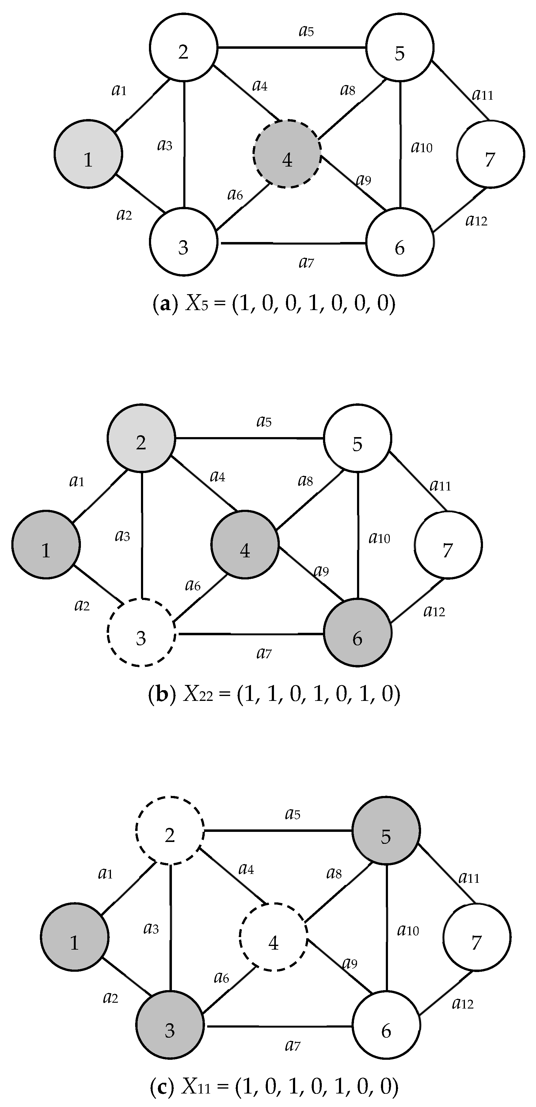
| X: | X = (X(1), X(2), …, X(|V|)) is a |V|-tuple node-based vector obtained from BAT such that its kth coordinate X(k) is represented whether node k is in the subnetwork with node 1 after the related cut. Note that X(1) = 1 and X(|V|) = 0 for all X. For example, X22 = (1, 1, 0, 1, 0, 1, 0) is the 22nd vector obtained from the BAT and denotes nodes 2, 4, and 6 are in the subnetwork with node 1 as shown in Figure 2. |
| S(X): | Node subset S(X) = {v ∊ V|X(v) = 1} ∪ {1}. For example, S(X22) = {1, 2, 4, 6} (see Figure 2) if X22 = (1, 1, 0, 1, 0, 1, 0) in Figure 1. |
| T(X): | Node subset T(X) = {v ∊ V|X(v) = 0} ∪ {n} = V − S(X). For example, T(X22) = {3, 5, 7} if X22 = (1, 1, 0, 1, 0, 1, 0) in Figure 1. |
| C(X): | Arc subset C(X) = ⌀ and {a ∊ E|for all a with one endpoint in S(X) and another one in T(X)} if X is infeasible or feasible, respectively. For example, C(X22) = ⌀ and C(X24) = {a5, a8, a10, a12} because X22 = (1, 1, 0, 1, 0, 1, 0) is infeasible, as shown in Figure 2, and X24 = (1, 1, 1, 1, 0, 1, 1) is feasible (Figure 3). |
| V(k): | Node subset V(k) = {j ∊ V|for all undirected arc a ∊ E from node k to node j ∊ V}. For example, V(2) = {1, 3, 4, 5} in Figure 1. |
| Pr(●): | Probability to have ● successfully, i.e., |
2.2. Assumptions
- Every individual node, denoted as v, is characterized by impeccable reliability. Furthermore, there exists at least one uncomplicated path that connects nodes 1 and n through node v.
- Every arc either operates effectively or is characterized by a failure. The probability of its occurrence operates independently, determined by a distribution grounded in empirical observations, data analysis, or rigorous testing.
- The system refrains from incorporating any loops or parallel arcs.
3. Overview of the MC, BAT, PLSA, and IET
3.1. MC and MC-Based Algorithms
3.2. BAT
| Rule 1: | The coordinate, denoted as X(i), exhibiting the inaugural zero value undergoes a transformation to one, while X(j) is set to zero for every j < i. |
| Rule 2: | In instances where X(i) = 1 for every i, the process is terminated, signifying the identification of all vectors. |
| Algorithm 1: Arc-based BAT [31] | |
| Input: | |E|. |
| Output: | All |E|-tuple binary-state vectors. |
| STEP 0. | Assign the values: i = 1 and X = 0. |
| STEP 1. | When X(ai) is 0, set both X(ai) and i to 1, then proceed to STEP 1. |
| STEP 2. | Halt if i = |E|. |
| STEP 3. | Increase i by 1, update X to 0, and return to STEP 1. |
3.3. Layers and PLSA
| Algorithm 2: PLSA [29] | |
| Input: | G(V, E) and vector X. |
| Output: | Whether nodes 1 and n is connected in G(X). |
| STEP 0. | Assign the values: i = 2 and L1 = {1}. |
| STEP 1. | Let Li = { v ∊ V|v ∉ (L1 ∪ L2 ∪ … ∪ Li−1) and u ∊ Li−1 are two endpoints of a ∊ E }. |
| STEP 2. | Halt and X is disconnected if Li = ⌀. |
| STEP 3. | Halt and X is connected if n ∊ ⌀. |
| STEP 4. | Increase i by one and return to STEP 1. |
3.4. IET
= Pr({a1, a2}) + Pr({a1, a3, a5}) + Pr({a2, a3, a4}) + Pr({a4, a5}) − [Pr({a1, a2, a3, a5}) + Pr({a1, a2, a3, a4}) + Pr(({a1, a2, a4, a5}) + Pr({a1, a2, a3, a4, a5}) + Pr({a1, a3, a4, a5}) + Pr({a2, a3, a4, a5})] + [Pr({a1, a2, a3, a4, a5}) + Pr({a1, a2, a3, a4, a5}) + Pr({a1, a2, a3, a4, a5}) + Pr({a1, a2, a3, a4, a5})] − Pr({a1, a2, a3, a4, a5}).
4. BAT-BASED NODE-BASED MC
4.1. Pseudocode
| Algorithm 3: Proposed BAT-Based Node-Based MC Algorithm [29,30,31] | |
| Input: | G(V, E), source node 1 and sink node n. |
| Output: | All MCs. |
| STEP 0. | Assign the values: X = 0, i = 1 and Ω = {{a ∊ E|a is adjacent to node 1}}. |
| STEP 1. | Reassign the values of X(i) and i to be 1 if X(i) = 0, and then proceed to STEP 4. |
| STEP 2. | Stop the process if u = |V|. |
| STEP 3. | Assign X(i) to 0, increment i by 1, and then proceed to STEP 1. |
| STEP 4. | If both G(S(X)) and G(T(X)) are connected subgraphs without isolated nodes, then let Ω = Ω ∪ {C(X)} because C(X) is an MC. Proceed to STEP 1. |
- The vector X transitions from being an arc-based |E|-tuple in Algorithm 1 to a node-based |V|-tuple.
- An additional STEP 4 is incorporated to identify the MC subsequent to acquiring a new iteration of X.
4.2. Step-by-Step Example
| STEP 0. | Assign the values: X = 0, i =1 and Ω = {{a1, a2}}. |
| STEP 1. | Given that X(1) = 0, set it to 1, assign i as 1, and proceed to STEP 4. |
| STEP 4. | Given that both G(S(X)) and G(T(X)) are connected, where S(X) = {1, 2} and T(X) = {3, 4, 5, 6, 7}, C(X) is defined as an MC with C(X) = {a2, a3, a4, a5}. Consequently, let Ω be updated to Ω = Ω ∪ {C(X)}, resulting in Ω = {{a1, a2}, {a2, a3, a4, a5}}. Now, proceed to STEP 1. |
| : | |
| : | |
| STEP 1. | In X = (1, 1, 0, 0, 0, 0, 0), since X(3) = 0, we update X(3) to 1 and set i to 1. Consequently, X becomes (1, 1, 1, 0, 0, 0, 0). Now, proceed to STEP 4. |
| STEP 4. | Given that G(S(X)) is disconnected, C(X) does not qualify as an MC. Proceed to STEP 1, noting that S(X) = {1, 2, 3}. |
| : | |
| : | |
| STEP 2. | Because i = |V| = 7, halt. |
5. Proposed Novel Concepts
5.1. Renumber Nodes Based on the PLSA
| Algorithm 4: PLSA-based Renumber Nodes [29] | |
| Input: | G(V, E), source node 1 and sink node n. |
| Output: | All MCs. |
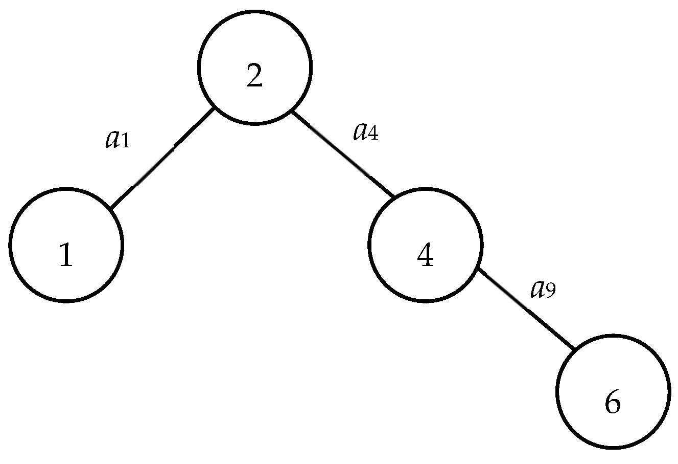
| STEP 0. | Implement Algorithm 2 to find L1, L2, …, Ll and λ(v) for all nodes v ∊ V. |
| STEP 1. | Renumber nodes such that nodes i < j if nodes i and j are in LƖ and Lφ, respectively, with Ɩ ≤ φ. |
| STEP 2. | Renumber nodes in each layer such that nodes i < j if nodes λ(i) > λ(i). |
5.2. Recursive Concept
5.3. Edge Nodes for Feasible Vectors
5.4. Isolated Nodes
- v is an element of S(X), but in G(S(X)) it fails to establish a path to node 1.
- Conversely, v belongs to T(X), but within G(T(X)) it is unable to connect to node n.
5.5. Fathom Vectors Based on Isolated Nodes
- Infeasibility of X1: Vector X1 is infeasible if node v1 is not an element of U(X).
- Inside Isolated Node Condition: X2 and its derivatives are infeasible if X2(v2) = 1 for every v in U(X) and X(u) = 0, where λ(u) < λ(v2). In this scenario, u is termed as an inside isolated node.
- Outside Isolated Node Condition: X2 and its derivatives are deemed infeasible if X2(v) = 0 for all v in the λ(v)th layer and λ(u) < λ(v2). Here, u is categorized as an outside isolated node. As an added nuance, the parent of X can be excluded from the recursive list.
- Future Isolated Node Condition: X2 and its derivatives are infeasible if X2(v2) = 1, X(u) = 0, both u and v2 are elements of U(X), u < v2, and U(X) is not connected. In this situation, u is defined as a future isolated node.
- Feasibility of X2: X2 is feasible if v2 is an element of U(X) and one of the subsequent conditions holds true:
- (1)
- v2 is an independent node.
- (2)
- v2 is a dependent node and X(u) = 1 for all nodes u that depended on v2.
- Efficiency in Connectivity Verification: The rules preclude the need for redundant connectivity checks for both X and all its derivatives X*, significantly reducing the computational overhead.
- Optimized Vector Generation: By establishing conditions for the infeasibility of vectors, the rules effectively minimize the unnecessary generation of vectors in the BAT, leading to a faster algorithm runtime.
- Systematic Fathoming: By incorporating these rules into the proposed algorithm, we ensure that the process will efficiently dismiss or validate not just individual vectors but entire sets of related vectors. This ensures a comprehensive, yet efficient, exploration of the solution space.
6. Proposed Algorithm
6.1. Pseudocode
| Algorithm 5: Proposed Node-based Recursive BAT [31] | |
| Input: | G(V, E), source node 1 and sink node n. |
| Output: | All MCs. |
| STEP 0. | Determine V(v) and λ(v) for all v ∊ V utilizing the PLSA. Initializing the values: set i to 2, j to 1, both N and N* to 2, X1 to (0), X2 to (1), S(X1) to {1}, S(X2) to {1, 2}, U(X1) to V(1), U(X2) to the difference between V(2) and {1}, and Ω to the set containing C(X1) and C(X2). |
| STEP 1. | Let X(v) = and S(X) = S(Xj) ∪ {(i+1)} based on Equations (3) and (4). |
| STEP 2. | If G(X) contains an isolated node denoted as u, then X and its offspring are deemed infeasible. Proceed to STEP 3. If not, advance to STEP 4. |
| STEP 3. | Eliminate Xj and proceed to STEP 4 if u is an outside isolated node. |
| STEP 4. | If node (i + 1) = 3 ∊ U(Xj), let U(X) = U(Xj) ∪ V((i + 1)) − S(X), Ω = Ω ∪ {C(X)}, N = N + 1 = 3, and XN = X. |
| STEP 5. | Increase j by 1 and proceed to STEP 1 if j < N*. |
| STEP 6. | If i < (|V| − 2), let i = i + 1, j = 1, N* = N, and go to STEP 1. Otherwise, terminate the process and Ω constitutes a complete MC set. |
6.2. Step-by-Step Example
| STEP 0. | Determine V(v) and λ(v) for all v ∊ V as shown in Table 4 and Table 5; let i = 2, j = 1, (|V| − 2) = 5, X1 = (0), S(X1) = {1}, U(X1) = V(1), X2 = (1), S(X2) = {1, 2}, U(X2) = V(2) − {1} = {3, 4, 5}, N = N* = 2, and Ω = {C(X1), C(X2)} = {{a1, a2}, {a2, a3, a4, a5}}. |
| STEP 1. | Let X(v) = , i.e., X = (0, 1), and S(X) = S(Xj) ∪ {(i + 1)} = {1, 3}. |
| STEP 2. | Because G(X) has no isolated nodes, proceed to STEP 4. |
| STEP 4. | Because node (i + 1) = 3 ∊ U(Xj), X is feasible and let U(X) = U(Xj) ∪ V((i + 1)) − S(X) = {2, 3} ∪ {1, 2, 4, 6} − {1, 3} = {2, 4, 6}, Ω = Ω ∪ {C(X)} = {{a1, a2}, {a2, a3, a4, a5}, {a1, a3, a6, a7}}, N = N + 1 = 3, and XN = X. |
| STEP 5. | Because j = 1 < N* = 2, let j = j + 1 = 2, and go to STEP 1. |
| STEP 1. | Let X(v) = , i.e., X = (1, 1), and S(X) = S(X2) ∪ {(2 + 1)} = {1, 2, 3}. |
| STEP 2. | Because there are no isolated nodes in G(X), go to STEP 4. |
| STEP 4. | Because node (i + 1) = 3 ∊ U(Xj), let U(X) = U(X2) ∪ V(3) − S(X) = {4, 5, 6}, Ω = Ω ∪ {C(X)} = { {a1, a2}, {a2, a3, a4, a5}, {a1, a3, a6, a7}, {a4, a5, a6, a7} }, N = N + 1 = 4, and XN = X4 = X. |
| STEP 5. | Because j = N* = 2, go to STEP 6. |
| STEP 6. | Because i = 2 < (|V| − 2) = 5, let i = i + 1 = 3, j = 1, N* = N = 4, and go to STEP 1. |
| STEP 1. | Let X(v) = , i.e., X = (0, 0, 1), and S(X) = S(Xj) ∪ {(i + 1)} = {1, 4}. |
| STEP 2. | Because node 4 is isolated, X and its offspring are all infeasible and go to STEP 3. |
| STEP 3. | Because node 4 is isolated outside, remove X1 and go to STEP 5. |
| STEP 5. | Because j = 1 < N* = 4, let j = j + 1 = 2 and go to STEP 1. |
| : | |
| Assume that i = 5, j = 12, N* = 10, and N = 4. | |
| STEP 1. | Let X(v) = , i.e., X = (1, 1, 1, 1, 1), and S(X) = S(Xj) ∪ {(i + 1)} = {1, 2, 3, 4, 5, 6}. |
| STEP 2. | Because there are no isolated nodes in G(X), go to STEP 4. |
| STEP 4. | Because node (i + 1) = 6 ∊ U(Xj) is connected, let U(X) = U(X2) ∪ V(3) − S(X) = {7}, Ω = Ω ∪ {C(X)}, N = N + 1 = 5, XN = X, and go to STEP 5. |
| STEP 5. | Because j = N* = 12, go to STEP 6. |
| STEP 6. | Because i = (|V| − 2) = 5, halt and all MCs are found in Ω = {{a1, a2}, {a2, a3, a4, a5}, {a1, a3, a6, a7}, {a4, a5, a6, a7}, {a2, a3, a5, a6, a8, a9}, {a1, a3, a4, a7, a8, a9}, {a5, a7, a8, a9}, {a2, a3, a4, a8, a10, a11}, {a4, a6, a7, a8, a10, a11}, {a2, a3, a6, a9, a10, a11}, {a7, a9, a10, a11}, {a1, a3, a6, a9, a10, a12}, {a4, a6, a7, a8, a10, a11}, {a4, a5, a6, a9, a12}, {a5, a8, a10, a12}, {a11, a12}}. |
6.3. Computation Experiments
7. Conclusions
- It pioneers a recursive approach within the realm of BAT algorithms aimed at MC extraction.
- The algorithm melds the agility of recursive BAT—enabling O(1) vector generation—with a strategic node renumbering scheme. This amalgamation aids in the early identification and pruning of infeasible vectors and their progeny, courtesy of the isolated node concept.
- The novel introduction of “edge nodes” further trims the computational overheads associated with feasibility verification of vectors.
Author Contributions
Funding
Data Availability Statement
Conflicts of Interest
Acronyms
| MC | Minimal cut |
| MP | Minimal path |
| DFS | depth-first search |
| IET | Inclusion–exclusion technology |
| BAT | Binary-addition-tree algorithm [28] |
| PLSA | Path-based layered-search algorithm |
Nomenclature
| Reliability | This denotes the probabilistic connection between nodes 1 and n. |
| Cut | A subset of arcs; when removed, it divides the entire graph or network into two separated subgraphs. |
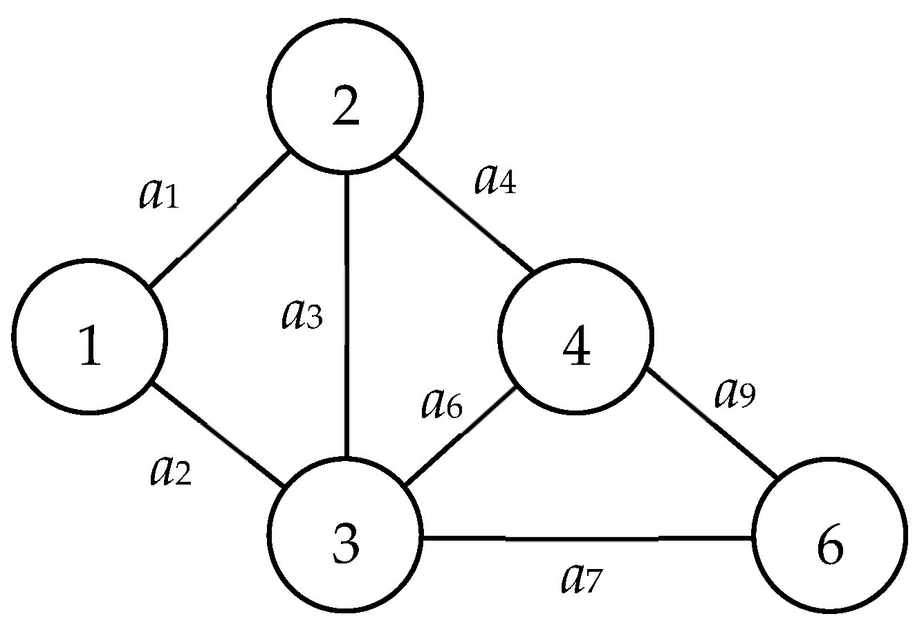
| MC | A distinctive cut between nodes 1 and n that lacks any superfluous arc; its excision does not affect other MCs. In Figure 1, while {a4, a5, a6, a7} exemplifies an MC, {a4, a5, a6} represents neither a cut nor an MC. Conversely, {a2, a4, a5, a6, a7} manifests as a cut, but the arc a2 renders it redundant, thus, not qualifying it as an MC. |
| MP | A simple path transitioning from node 1 to n, devoid of any redundant arc. Illustrated in Figure 1, {a2, a7, a12} is an MP, whereas {a2, a7} does not constitute a path or an MP. However, {a1, a2, a7, a12} stands as an MP but includes the superfluous arc a1. |
| Isolated node | Within the context of X, a node v is deemed isolated if there exists no pathway from node 1 to node v or from node v to node n in the graphs G(S(X)) and G(T(X)), respectively. A case in point from Figure 1: node 3, within X22 = (1, 1, 0, 1, 0, 1, 0), is isolated since it belongs to T(X22) but lacks connectivity to node 7 in G(T(X22)). |
| Edge node | In the context of X, a node in U(X) = T(X) ∩ {all nodes adjacent to arcs in C(X)} receives the designation of an “edge node” if it is encapsulated within U(X). Drawing from Figure 1, nodes 5 and 7 both qualify as edge nodes in the set X24 = (1, 1, 1, 1, 0, 1, 1). |
| Feasible/Infeasible Vector | A vector, X, predicated on nodes, is termed “feasible” if C(X) corresponds to an MC and no isolated nodes exist within X. An instance from Figure 1 can be discerned in vectors X22 = (1, 1, 0, 1, 0, 1, 0) and X24 = (1, 1, 1, 1, 0, 1, 1). The former is infeasible due to the presence of an isolated node, node 3, whereas the latter is feasible owing to the absence of isolated nodes. |
References
- Niu, Y.F. Performance measure of a multi-state flow network under reliability and maintenance cost considerations. Reliab. Eng. Syst. Saf. 2021, 215, 107822. [Google Scholar] [CrossRef]
- Wang, W.C.; Zhang, Y.; Li, Y.X.; Hu, Q.; Liu, C.; Liu, C. Vulnerability analysis method based on risk assessment for gas transmission capabilities of natural gas pipeline networks. Reliab. Eng. Syst. Saf. 2022, 218, 108150. [Google Scholar] [CrossRef]
- Ma, G.; Huang, Y.; Li, J. Bayesian Network Analysis of Explosion Events at Petrol Stations. In Risk Analysis of Vapour Cloud Explosions for Oil and Gas Facilities; Springer: Singapore, 2019; pp. 191–217. [Google Scholar]
- Honqqum, L.; Xianlin, H.; Gao, X.Z.; Xiaojun, B.; Hang, Y. Stability analysis of the simplest Takagi-Sugeno fuzzy control system using circle criterion. J. Syst. Eng. Electron. 2007, 18, 311–319. [Google Scholar] [CrossRef]
- He, R.; Deng, J.; Lai, L.L. Reliability evaluation of communication-constrained protection systems using stochastic-flow network models. IEEE Trans. Smart Grid 2017, 9, 2371–2381. [Google Scholar]
- Aven, T. Availability evaluation of oil/gas production and transportation systems. Reliab. Eng. 1987, 18, 35–44. [Google Scholar] [CrossRef]
- Kakadia, D.; Ramirez-Marquez, J.E. Quantitative approaches for optimization of user experience based on network resilience for wireless service provider networks. Reliab. Eng. Syst. Saf. 2020, 193, 106606. [Google Scholar] [CrossRef]
- Yeh, W.C. A simple algorithm for evaluating the k-out-of-n network reliability. Reliab. Eng. Syst. Saf. 2004, 83, 93–101. [Google Scholar] [CrossRef]
- Yang, Y.; Wang, S.; Xu, W.; Wei, K. Reliability evaluation of wireless multimedia sensor networks based on instantaneous availability. Int. J. Distrib. Sens. Netw. 2018, 14, 1550147718810692. [Google Scholar] [CrossRef]
- Gongora-Svartzman, G.; Ramirez-Marquez, J.E. Social cohesion: Mitigating societal risk in case studies of digital media in Hurricanes Harvey, Irma, and Maria. Risk Anal. 2022, 42, 1686–1703. [Google Scholar] [CrossRef]
- Colbourn, C.J. The Combinatorics of Network Reliability; Oxford University Press, Inc.: New York, NY, USA, 1987. [Google Scholar]
- Shier, D.R. Network Reliability and Algebraic Structures; Clarendon Press: New York, NY, USA, 1991. [Google Scholar]
- Levitin, G. The Universal Generating Function in Reliability Analysis and Optimization; Springer: Berlin/Heidelberg, Germany, 2005. [Google Scholar]
- Pandey, M.; Zuo, M.J.; Moghaddass, R.; Tiwari, M.K. Selective maintenance for binary systems under imperfect repair. Reliab. Eng. Syst. Saf. 2013, 113, 42–51. [Google Scholar] [CrossRef]
- Ramirez-Marquez, J.E. Approximation of minimal cut sets for a flow network via evolutionary optimization and data mining techniques. Int. J. Perform Abil. Eng. 2011, 7, 21. [Google Scholar]
- Forghani-elahabad, M.; Kagan, N. Reliability evaluation of a stochastic-flow network in terms of minimal paths with budget constraint. IISE Trans. 2019, 51, 547–558. [Google Scholar] [CrossRef]
- Wang, C.; Xing, L.; Levitin, G. Reliability analysis of multi-trigger binary systems subject to competing failures. Reliab. Eng. Syst. Saf. 2013, 111, 9–17. [Google Scholar] [CrossRef]
- Larsen, E.M.; Ding, Y.; Li, Y.F.; Zio, E. Definitions of generalized multi-performance weighted multi-state K-out-of-n system and its reliability evaluations. Reliab. Eng. Syst. Saf. 2020, 199, 105876. [Google Scholar] [CrossRef]
- Moghaddass, R.; Zuo, M.J. An integrated framework for online diagnostic and prognostic health monitoring using a multistate deterioration process. Reliab. Eng. Syst. Saf. 2014, 124, 92–104. [Google Scholar] [CrossRef]
- Levitin, G. A universal generating function approach for the analysis of multi-state systems with dependent elements. Reliab. Eng. Syst. Saf. 2004, 84, 285–292. [Google Scholar] [CrossRef]
- Niu, Y.F.; Song, Y.F.; Xu, X.Z. Budget optimization for a multi-distribution multi-state logistics network with reliability consideration. Qual. Technol. Quant. Manag. 2023, 20, 528–544. [Google Scholar] [CrossRef]
- Levitin, G.; Gertsbakh, I.; Shpungin, Y. Evaluating the damage associated with intentional supply deprivation in multi-commodity network. Reliab. Eng. Syst. Saf. 2013, 119, 11–17. [Google Scholar] [CrossRef]
- Lin, S.; Jia, L.; Zhang, H.; Zhang, P. Reliability of high-speed electric multiple units in terms of the expanded multi-state flow network. Reliab. Eng. Syst. Saf. 2022, 225, 108608. [Google Scholar] [CrossRef]
- Zhou, J.; Coit, D.W.; Felder, F.A.; Wang, D. Resiliency-based restoration optimization for dependent network systems against cascading failures. Reliab. Eng. Syst. Saf. 2021, 207, 107383. [Google Scholar] [CrossRef]
- Khan, A.; Bonchi, F.; Gullo, F.; Nufer, A. Conditional reliability in uncertain graphs. IEEE Trans. Knowl. Data Eng. 2018, 30, 2078–2092. [Google Scholar] [CrossRef]
- Yeh, W.C. Search for MC in modified networks. Comput. Oper. Res. 2001, 28, 177–184. [Google Scholar] [CrossRef]
- Zuo, M.J.; Tian, Z.; Huang, H.Z. An efficient method for reliability evaluation of multistate networks given all minimal path vectors. IIE Trans. 2007, 39, 811–817. [Google Scholar] [CrossRef]
- Yeh, W.C. Novel Binary-Addition Tree Algorithm (BAT) for Binary-State Network Reliability Problem. Reliab. Eng. Syst. Saf. 2020, 208, 107448. [Google Scholar] [CrossRef]
- Yeh, W.C. Novel Recursive Inclusion-Exclusion Technology Based on BAT and MPs for Heterogeneous-Arc Binary-State Network Reliability Problems. Reliab. Eng. Syst. Saf. 2023, 231, 107917. [Google Scholar] [CrossRef]
- Yeh, W.C. A revised layered-network algorithm to search for all d-minpaths of a limited-flow acyclic network. IEEE Trans. Reliab. 1998, 47, 436–442. [Google Scholar]
- Available online: https://drive.google.com/file/d/1cMkbIXqI2QlPu70oR42EgLxMMwEM_REz/view (accessed on 11 January 2023).


| i | Li | Li+1 |
|---|---|---|
| 1 | {1} | {2} |
| 2 | {2} | {4} |
| 3 | {4} | {6} |
| 4 | {6} |
| i | Xi | S(Xi) | T(Xi) | C(X) | U(Xi) |
|---|---|---|---|---|---|
| 1 | (1, 0, 0, 0, 0, 0, 0) | {1} | {2, 3, 4, 5, 6, 7} | {a1, a2} | {2, 3} |
| 2 | (1, 1, 0, 0, 0, 0, 0) | {1, 2} | {3, 4, 5, 6, 7} | {a2, a3, a4, a5} | {3, 4, 5} |
| 3 | (1, 0, 1, 0, 0, 0, 0) | {1, 3} | {2, 4, 5, 6, 7} | {a1, a3, a6, a7} | {2, 4, 6} |
| 4 | (1, 1, 1, 0, 0, 0, 0) | {1, 2, 3} | {4, 5, 6, 7} | {a4, a5, a6, a7} | {4, 5, 6} |
| 5 | (1, 0, 0, 1, 0, 0, 0) | {1, 4} | |||
| 6 | (1, 1, 0, 1, 0, 0, 0) | {1, 2, 4} | {3, 5, 6, 7} | {a2, a3, a5, a6, a8, a9} | {3, 5, 6} |
| 7 | (1, 0, 1, 1, 0, 0, 0) | {1, 3, 4} | {2, 5, 6, 7} | {a1, a3, a4, a7, a8, a9} | {2, 5, 6} |
| 8 | (1, 1, 1, 1, 0, 0, 0) | {1, 2, 3, 4} | {5, 6, 7} | {a5, a7, a8, a9} | {5, 6} |
| 9 | (1, 0, 0, 0, 1, 0, 0) | {1, 5} | |||
| 10 | (1, 1, 0, 0, 1, 0, 0) | {1, 2, 5} | {3, 4, 6, 7} | {a2, a3, a4, a8, a10, a11} | {3, 4, 6, 7} |
| 11 | (1, 0, 1, 0, 1, 0, 0) | {1, 3, 5} | |||
| 12 | (1, 1, 1, 0, 1, 0, 0) | {1, 2, 3, 5} | {4, 6, 7} | {a4, a6, a7, a8, a10, a11} | {4, 6, 7} |
| 13 | (1, 0, 0, 1, 1, 0, 0) | {1, 4, 5} | |||
| 14 | (1, 1, 0, 1, 1, 0, 0) | {1, 2, 4, 5} | {3, 6, 7} | {a2, a3, a6, a9, a10, a11} | {3, 6, 7} |
| 15 | (1, 0, 1, 1, 1, 0, 0) | {1, 3, 4, 5} | |||
| 16 | (1, 1, 1, 1, 1, 0, 0) | {1, 2, 3, 4, 5} | {6, 7} | {a7, a9, a10, a11} | {6, 7} |
| 17 | (1, 0, 0, 0, 0, 1, 0) | {1, 6} | |||
| 18 | (1, 1, 0, 0, 0, 1, 0) | {1, 2, 6} | |||
| 19 | (1, 0, 1, 0, 0, 1, 0) | {1, 3, 6} | {2, 4, 5, 7} | {a1, a3, a6, a9, a10, a12} | {2, 4, 5, 7} |
| 20 | (1, 1, 1, 0, 0, 1, 0) | {1, 2, 3, 6} | {4, 5, 7} | {a4, a6, a7, a8, a10, a11} | {4, 5, 7} |
| 21 | (1, 0, 0, 1, 0, 1, 0) | {1, 4, 6} | |||
| 22 | (1, 1, 0, 1, 0, 1, 0) | {1, 2, 4, 6} | |||
| 23 | (1, 0, 1, 1, 0, 1, 0) | {1, 3, 4, 6} | {2, 5, 7} | {a4, a5, a6, a9, a12} | {2, 5, 7} |
| 24 | (1, 1, 1, 1, 0, 1, 0) | {1, 2, 3, 4, 6} | {5, 7} | {a5, a8, a10, a12} | {5, 7} |
| 25 | (1, 0, 0, 0, 1, 1, 0) | {1, 5, 6} | |||
| 26 | (1, 1, 0, 0, 1, 1, 0) | {1, 2, 5, 6} | |||
| 27 | (1, 0, 1, 0, 1, 1, 0) | {1, 3, 5, 6} | |||
| 28 | (1, 1, 1, 0, 1, 1, 0) | {1, 2, 3, 5, 6} | |||
| 29 | (1, 0, 0, 1, 1, 1, 0) | {1, 4, 5, 6} | |||
| 30 | (1, 1, 0, 1, 1, 1, 0) | {1, 2, 4, 5, 6} | |||
| 31 | (1, 0, 1, 1, 1, 1, 0) | {1, 3, 4, 5, 6} | |||
| 32 | (1, 1, 1, 1, 1, 1, 0) | {1, 2, 3, 4, 5, 6} | {7} | {a11, a12} |
| i | 1 | 2 | 3 | 4 | |||
| L(i) | {1} | {2, 3} | {4, 5, 6} | {7} | |||
| v | 1 | 2 | 3 | 4 | 5 | 6 | 7 |
| λ(v) | 1 | 2 | 2 | 3 | 3 | 3 | 4 |
| j | Xj = X1,j | S(Xj) | U(Xj) | C(Xj) |
|---|---|---|---|---|
| 1 | (0) | {1} | {2, 3} | {a1, a2} |
| 2 | (1) | {1, 2} | {3, 4, 5} | {a2, a3, a4, a5} |
| J | Xi = X1,j | S(Xi) | U(Xi) | i | j | Xi = X2,j | S(Xi) | U(Xi) | C(Xi) |
|---|---|---|---|---|---|---|---|---|---|
| 1 | (0) | {1} | {2, 3} | 3 | 1 | (0, 1) | {1, 3} | {2, 4, 6} | {a1, a3, a6, a7} |
| 2 | (1) | {1, 2} | {3, 4, 5} | 4 | 2 | (1, 1) | {1, 2, 3} | {4, 5, 6} | {a4, a5, a6, a7} |
| i | Xi | S(Xi) | U(Xi) | i | Xi | S(Xi) | U(Xi) | C(Xi) |
|---|---|---|---|---|---|---|---|---|
| 1 | (0) | {1} | {2, 3} | 5 | (0, 0, 1) | {1, 4}D | ||
| 2 | (1) | {1, 2} | {3, 4, 5} | 6 | (1, 0, 1) | {1, 2, 4} | {4, 5, 6} | {a2, a3, a5, a6, a8, a9} |
| 3 | (0, 1) | {1, 3} | {2, 4, 6} | 7 | (0, 1, 1) | {1, 3, 4} | {2, 5, 6} | {a1, a3, a4, a7, a8, a9} |
| 4 | (1, 1) | {1, 2, 3} | {4, 5, 6} | 8 | (1, 1, 1) | {1, 2, 3, 4} | {5, 6} | {a5, a7, a8, a9} |
| I | Xi | S(Xi) | U(Xi) | i | Xi | S(Xi) | U(Xi) | C(Xi) |
|---|---|---|---|---|---|---|---|---|
| 1 | (0) | {1} | {2, 3} | 9 | (0, 0, 0, 1) | {1, 5}D | ||
| 2 | (1) | {1, 2} | {3, 4, 5} | 10 | (1, 0, 0, 1) | {1, 2, 5} | {3, 4, 6, 7} | {a2, a3, a4, a8, a10, a11} |
| 3 | (0, 1) | {1, 3} | {2, 4, 6} | 11 | (0, 1, 0, 1) | {1, 3, 5}D | ||
| 4 | (1, 1) | {1, 2, 3} | {4, 5, 6} | 12 | (1, 1, 0, 1) | {1, 2, 3, 5} | {4, 6, 7} | {a4, a6, a7, a8, a10, a11} |
| 5 | (0, 0, 1) | {1, 4}D | 13 | (0, 0, 1, 1) | {1, 4, 5}D | |||
| 6 | (1, 0, 1) | {1, 2, 4} | {4, 5, 6} | 14 | (1, 0, 1, 1) | {1, 2, 4, 5} | {3, 6, 7} | {a2, a3, a6, a9, a10, a11} |
| 7 | (0, 1, 1) | {1, 3, 4} | {2, 5, 6} | 15 | (0, 1, 1, 1) | {1, 3, 4, 5}D | ||
| 8 | (1, 1, 1) | {1, 2, 3, 4} | {5, 6} | 16 | (1, 1, 1, 1) | {1, 2, 3, 4, 5} | {6, 7} | {a7, a9, a10, a11} |
| i | Xi | S(Xi) | U(Xi) | i | Xi | S(Xi) | C(Xi) |
|---|---|---|---|---|---|---|---|
| 1 | (0) | {1} | {2, 3} | 17 | (0, 0, 0, 0, 1) | {1, 6}D | |
| 2 | (1) | {1, 2} | {3, 4, 5} | 18 | (1, 0, 0, 0, 1) | {1, 2, 6}D | |
| 3 | (0, 1) | {1, 3} | {2, 4, 6} | 19 | (0, 1, 0, 0, 1) | {1, 3, 6} | {a1, a3, a6, a9, a10, a12} |
| 4 | (1, 1) | {1, 2, 3} | {4, 5, 6} | 20 | (1, 1, 0, 0, 1) | {1, 2, 3, 6} | {a4, a6, a7, a8, a10, a11} |
| 5 | (0, 0, 1) | {1, 4}D | 21 | (0, 0, 1, 0, 1) | {1, 4, 6}D | ||
| 6 | (1, 0, 1) | {1, 2, 4} | {4, 5, 6} | 22 | (1, 0, 1, 0, 1) | {1, 2, 4, 6}D | |
| 7 | (0, 1, 1) | {1, 3, 4} | {2, 5, 6} | 23 | (0, 1, 1, 0, 1) | {1, 3, 4, 6} | {a4, a5, a6, a9, a12} |
| 8 | (1, 1, 1) | {1, 2, 3, 4} | {5, 6} | 24 | (1, 1, 1, 0, 1) | {1, 2, 3, 4, 6} | {a5, a8, a10, a12} |
| 9 | (0, 0, 0, 1) | {1, 5}D | 25 | (0, 0, 0, 1, 1) | {1, 5, 6}D | ||
| 10 | (1, 0, 0, 1) | {1, 2, 5} | {3, 4, 6, 7} | 26 | (1, 0, 0, 1, 1) | {1, 2, 5, 6}D | |
| 11 | (0, 1, 0, 1) | {1, 3, 5}D | 27 | (0, 1, 0, 1, 1) | {1, 3, 5, 6}D | ||
| 12 | (1, 1, 0, 1) | {1, 2, 3, 5} | {4, 6, 7} | 28 | (1, 1, 0, 1, 1) | {1, 2, 3, 5, 6}D | |
| 13 | (0, 0, 1, 1) | {1, 4, 5}D | 29 | (0, 0, 1, 1, 1) | {1, 4, 5, 6}D | ||
| 14 | (1, 0, 1, 1) | {1, 2, 4, 5} | {3, 6, 7} | 30 | (1, 0, 1, 1, 1) | {1, 2, 4, 5, 6}D | |
| 15 | (0, 1, 1, 1) | {1, 3, 4, 5}D | 31 | (0, 1, 1, 1, 1) | {1, 3, 4, 5, 6}D | ||
| 16 | (1, 1, 1, 1) | {1, 2, 3, 4, 5} | {6, 7} | 32 | (1, 1, 1, 1, 1) | {1, 2, 3, 4, 5, 6} | {a11, a12} |
| Fig. | n | m | c | TNBA | TRBAT |
|---|---|---|---|---|---|
| 1 | 4 | 5 | 4 | 0 | 0 |
| 2 | 6 | 8 | 9 | 0 | 0 |
| 3 | 5 | 8 | 8 | 0 | 0 |
| 4 | 6 | 9 | 9 | 0 | 0 |
| 5 | 9 | 12 | 28 | 0 | 0 |
| 6 | 7 | 14 | 25 | 0 | 0 |
| 7 | 11 | 21 | 133 | 0 | 0 |
| 8 | 9 | 13 | 24 | 0 | 0 |
| 9 | 8 | 12 | 19 | 0 | 0 |
| 10 | 9 | 14 | 25 | 0 | 0 |
| 11 | 7 | 12 | 20 | 0 | 0 |
| 12 | 8 | 13 | 29 | 0 | 0 |
| 14 | 21 | 26 | 528 | 0.041 | 0.018 |
| 15 | 9 | 14 | 25 | 0 | 0 |
| 16 | 10 | 21 | 104 | 0 | 0 |
| 17 | 18 | 27 | 1249 | 0.159 | 0.022 |
| 19 | 20 | 30 | 7376 | 0.436 | 0.093 |
| 20 | 16 | 24 | 105 | 0.001 | 0.001 |
| 21 | 16 | 30 | 644 | 0.083 | 0.012 |
| 22 | 13 | 22 | 214 | 0.003 | 0.001 |
Disclaimer/Publisher’s Note: The statements, opinions and data contained in all publications are solely those of the individual author(s) and contributor(s) and not of MDPI and/or the editor(s). MDPI and/or the editor(s) disclaim responsibility for any injury to people or property resulting from any ideas, methods, instructions or products referred to in the content. |
© 2024 by the authors. Licensee MDPI, Basel, Switzerland. This article is an open access article distributed under the terms and conditions of the Creative Commons Attribution (CC BY) license (https://creativecommons.org/licenses/by/4.0/).
Share and Cite
Yeh, W.-C.; Yang, G.; Huang, C.-L. A New Node-Based Algorithm for Identifying the Complete Minimal Cut Set. Electronics 2024, 13, 603. https://doi.org/10.3390/electronics13030603
Yeh W-C, Yang G, Huang C-L. A New Node-Based Algorithm for Identifying the Complete Minimal Cut Set. Electronics. 2024; 13(3):603. https://doi.org/10.3390/electronics13030603
Chicago/Turabian StyleYeh, Wei-Chang, Guangyi Yang, and Chia-Ling Huang. 2024. "A New Node-Based Algorithm for Identifying the Complete Minimal Cut Set" Electronics 13, no. 3: 603. https://doi.org/10.3390/electronics13030603
APA StyleYeh, W.-C., Yang, G., & Huang, C.-L. (2024). A New Node-Based Algorithm for Identifying the Complete Minimal Cut Set. Electronics, 13(3), 603. https://doi.org/10.3390/electronics13030603