A Study on Fractional Power-Law Applications and Approximations

Abstract

The frequency response of the fractional-order power-law filter can be approximated by different techniques, which eventually affect the expected performance. Fractional-order control systems introduce many benefits for applications like compensators to achieve robust frequency and additional degrees of freedom in the tuning process. This paper is a comparative study of five of these approximation techniques. The comparison focuses on their magnitude error, phase error, and implementation complexity. The techniques under study are the Carlson, continued fraction expansion (CFE), Padé, Charef, and MATLAB curve-fitting tool approximations. Based on this comparison, the recommended approximation techniques are the curve-fitting MATLAB tool and the continued fraction expansion (CFE). As an application, a low-pass power-law filter is realized on a field-programmable analog array (FPAA) using two techniques, namely the curve-fitting tool and the CFE. The experiment aligns with and validates the numerical results.

1. Introduction

Fractional calculus is a generalization of integration and differentiation to non-integer orders, as it contains the rules that govern processes involving non-integer orders [1,2]. The fractional calculus field started with a question asked by L’Hôpital, a French mathematician, to Leibniz about the derivative of $d^{1/2}y\left(x\right)/d{x}^{1/2}$. The answer was, “It will lead to a paradox, from which practical consequences would one day be drawn” [1,3]. In practical applications, fractional calculus introduces invisible information in classical calculus, as fractional-order derivatives are more informative compared to integer-order ones [4]. Also, gradual changes happen when the orders are non-integers.

Non-integer-order signal processing has attracted significant research interest in many applications, such as filters and oscillators, chaotic systems, sensor systems, and control systems [5,6,7]. In addition, numerous physical phenomena are known to exhibit a fractional power function dependence on frequency or, equivalently, a fractional slope on the log-log plot, including certain types of electrical noise [8], the relaxation behavior of polarized impedances in dielectrics [9], transmission lines, and the spectral densities of music [10].

The area of fractional-order control has attracted significant research interest due to the additional degrees of freedom in the tuning process [11]. Many fractional-order filter applications were investigated, such as the design of a current feedback operational amplifier (CFOA)-based inverse filter in [6]. Applications of non-integer-order signal processing systems require levels of accuracy and sensitivity that can be achieved by the current feedback operational amplifier implementation of the power-law filters approximated by the curve-fitting-based technique [12]. Also, applications of analog pseudo-differential fractional frequency filters use the Butterworth approximation of the fractional order ($2+\alpha$) [13]. Furthermore, many fractional-order oscillators have been widely studied in [14,15].

The power-law filter is a new category of fractional-order filters that can be realized without using the fractional-order Laplacian operator, thereby eliminating the need for fractional-order elements when realizing this class of filters [16,17]. The fractional-order lead/lag compensator provides additional degrees of freedom in the tuning process in the fractional-order control area [18]. One of the forms of the fractional-order lead/lag compensator involves raising the integer-order counterpart to a non-integer-order power, transforming it into a type of power-law filter. The fractional-order lead/lag compensator shapes the open- or closed-loop response to achieve the desired stability, robustness, and other performance specifications [11,19]. In control systems, achieving robust frequency compensation is a goal discussed in [16,20], particularly when dealing with plants with uncertain poles, where selecting compensator parameters plays a crucial role. This type of lead/lag compensator is realized by approximating the fractional-order transfer function using the Padé approximation [11].

The dynamic behavior of fractional transfer functions can be approximated using integer transfer functions or digital transfer functions [21,22]. Approximations are helpful in numerical methods for solving fractional differential equations. Methods for solving integer differential equations are more widely available in commercial software [21]. For hardware implementations of fractional controllers, integer transfer functions are easier and cheaper to implement [21]. This paper focuses on rational approximation techniques for the applications of fractional power-law forms.

The concept of the mother function was introduced in [16] as $H_m\left(s\right)$, mother function based on power law. Considering $H_f\left(s^{\alpha }\right)=H_m\left(s\right){|}_{s\to s^{\alpha }}$ leads to a clear conclusion regarding the relation between the fractional-order function and the mother function based on power law. The mother function is raised to a non-integer number $\alpha$. The circuit realization of $s^{\alpha }$ needs a fractional-order element, which is not commercially available. So, it is implemented using the fractional-order capacitor approximation through Cauer or Foster techniques or fractional-order inductors achieved by adding Generalized Impedance Converters (GICs) to the Cauer or Foster structure [16,23]. A different approach is to approximate the fractional-order Laplacian operator through an integer-order transfer function, using rational integer-order approximation techniques to obtain the function $H\left(s\right)\cong H_f\left(s^{\alpha }\right){|}_{s^{\alpha }\to T\left(s\right)}$. The mother function’s representation gives us the magnitude and phase responses, expressed as $|H_f\left(\omega \right)|={\left[|H_m\left(\omega \right)|\right]}^{\alpha }$ and $\angle H_f\left(\omega \right)=\alpha \times \angle H_m\left(\omega \right)$. This leads to the next step of approximating ${\left[H_m\left(\omega \right)\right]}^{\alpha }$ after obtaining the frequency response using appropriate magnitude and phase curve-fitting techniques. Many approximation tools, like Oustaloup, Matsuda, and continued fraction expansion, are incapable of realizing the power-law filters’ transfer function, as it is based on approximating the fractional-order Laplacian operator itself $s^{\alpha }$ [11,24]. Other approximations like the stability boundary locus can improve stability preservation and achieve acceptable time and frequency response matching for fractional-order systems [25].

This paper compares some of these approximations by modifying them to approximate the whole filter transfer function of power-law filters instead of approximating the Laplacian operator only. The challenge in approximating this type of transfer function is that the fractional order appears in both the numerator and denominator [16]. Therefore, the power-law concept involves realizing transfer functions without fractional-order elements. A fractional-order low-pass power-law filter is realized using the curve-fitting and the CFE approximation techniques and implemented using the FPAA and the NI ELVIS II kit experimentally.Also, a fractional-order compensator is realized using the curve-fitting approximation technique and implemented as a software interface on the FPAA. This paper is organized as follows, The power-law filters are discussed in detail in Section 2, Section 3 shows the usage of the approximation techniques, Section 4 compares the different realizations, and Section 5 demonstrates the FPAA realization. Finally Section 6 concludes the comparison and the implementation observations.

2. Power-Law Functions

The power-law filter function is formed by raising the integer-order filter function to a non-integer exponent [24]. These filters are derived from the first- and second-order mother functions introduced in [16]. Also, the fractional-order lead/lag compensator is a power law filter. Hence, this paper focuses on first-order power-law filters and lead/lag compensators.

2.1. First-Order Power-Law Filters

The Power-Law low- and high-pass filters’ corresponding transfer functions are $H_{PL-LP}\left(s\right)$ and $H_{PL-HP}\left(s\right)$, respectively [16]:

$$H_{PL-LP}\left(s\right)={\left(\frac{{\omega }_0}{s+{\omega }_0}\right)}^{\alpha },$$

(1)

$$H_{PL-HP}\left(s\right)={\left(\frac{s}{s+{\omega }_0}\right)}^{\alpha },$$

(2)

where ($0<\alpha <1$) is the fractional order, and ${\omega }_0$ is the pole frequency. To obtain the magnitude and phase responses for each type, the following equations are utilized [16]:

$$|H_{PL-LP}\left(s\right)|=\frac{1}{{\left[{\left(\frac{\omega }{{\omega }_0}\right)}^2+1\right]}^{\alpha /2}},$$

(3)

$$\angle H_{PL-LP}\left(s\right)=-\alpha {tan}^{-1}\left(\frac{\omega }{{\omega }_0}\right),$$

(4)

$$|H_{PL-HP}\left(s\right)|=\frac{{\left(\frac{\omega }{{\omega }_0}\right)}^{\alpha }}{{\left[{\left(\frac{\omega }{{\omega }_0}\right)}^2+1\right]}^{\alpha /2}},$$

(5)

$$\angle H_{PL-HP}\left(s\right)=\alpha {tan}^{-1}\left(\frac{{\omega }_0}{\omega }\right).$$

(6)

The point at which the gain is attenuated by 3 dB from the DC gain is called the half-power frequency. And it can be determined by the pole frequency ${\omega }_o$ and the fractional order $\alpha$ [5]. Equation (7) shows the calculation of the half-power frequency and the corresponding phase for both low- and high-pass filters [16]:

$${\omega }_{h(-3dB)PL-LP}={\omega }_0\sqrt{2^{1/\alpha }-1},$$

(7a)

$$\angle H_{PL-LP}\left({\omega }_h\right)=-\alpha \times {tan}^{-1}\left(\sqrt{2^{1/\alpha }-1}\right),$$

(7b)

$${\omega }_{h(-3dB)PL-HP}=\frac{{\omega }_0}{\sqrt{2^{1/\alpha }-1}},$$

(7c)

$$\angle H_{PL-HP}\left({\omega }_h\right)=\alpha \times \left[\frac{\pi }{2}-{tan}^{-1}\left(\frac{1}{\sqrt{2^{1/\alpha }-1}}\right)\right].$$

(7d)

In Equations (7a) and (7c), the pole frequency determines the reference point, and the fractional order determines the distances, as for the low- and high-pass ${\omega }_h$ has equal distances in logarithmic scale around the pole frequency as shown in [5]:

$${\omega }_0=\sqrt{{\omega }_{h,(PL-LP)}\times {\omega }_{h,(PL-HP)}}.$$

(8)

The attenuation slope for the low-pass filter is $-20\alpha$ dB/dec, whereas for the high-pass filter, it is $20\alpha$ dB/dec [5]. The phase for the low-pass at very low frequencies is equal to zero, and it asymptotically tends to the value ($-\alpha \pi /2$) at very high frequencies. For the high-pass filter, the phase at very low frequencies tends to ($+\alpha \pi /2$), whereas at high frequencies, it tends to zero [16]. Raising the conventional filter functions to the non-integer exponent $\alpha$ gives an additional degree of freedom, allowing for precise adjustment of the filter’s characteristics, including the cut-off frequency and the transition slope from the passband to the stopband [24]. The frequency responses of the derived functions exhibit an attenuation gradient scaled by a factor equal to the order of the filter, in comparison to the corresponding response of the mother filter function [24].

2.2. Power-Law Lead/Lag Compensators

The corresponding transfer function of a lead/lag compensator is [11]:

$$C\left(s\right)=K\times {\left(\frac{1+\tau s}{1+x\tau s}\right)}^{\alpha },$$

(9)

where K is the DC compensator gain, $(\tau >0$) is the time constant, and ($x>0$) is the scaling factor of the time constant that determines the type of compensator (lead or lag) [11]. The zero frequency is (${\omega }_z=\frac{1}{\tau }$), and the pole frequency is (${\omega }_P=\frac{1}{x\tau }$). For implementing a fractional-order lead compensator, the zero frequency must be smaller than the pole frequency (${\omega }_z<{\omega }_p$), so the given condition must be achieved [11]:

$$(0<x<1),$$

(10)

and for implementing a fractional-order lag compensator, the opposite condition must be achieved, so [11]:

$$(x>1).$$

(11)

In forming the compensator type, the fractional order $\alpha$ represents a degree of freedom which is visible in the design flexibility standpoint [11]. The geometric mean of the pole and zero frequencies is given by (${\omega }_m=\sqrt{{\omega }_z\times {\omega }_P}$). Expressing the zero in terms of the pole yields:

$${\omega }_z=x\times {\omega }_P,$$

(12)

so ${\omega }_m$ can be written in terms of the characteristics of the compensator (x,$\tau$) [11]:

$${\omega }_m=\frac{1}{x^{1/2}\tau }.$$

(13)

The magnitude and phase responses are calculated using Equation (9) [11]:

$$\left|C\left(s\right)\right|=K\times {\left[\frac{1+{\left(\omega \tau \right)}^2}{1+{\left(x\omega \tau \right)}^2}\right]}^{\alpha /2},$$

(14a)

$$\angle C\left(s\right)=\alpha \times {tan}^{-1}\left[\frac{\omega \tau (1-x)}{1+x{\left(\omega \tau \right)}^2}\right].$$

(14b)

The gain ($K_m$) and phase (${\varphi }_m$) values at the ${\omega }_m$ frequency are [11]:

$$K_m=\frac{K}{x^{\alpha /2}},$$

(15a)

$${\varphi }_m=\alpha \times {sin}^{-1}\left(\frac{1-x}{1+x}\right).$$

(15b)

Therefore, the compensator’s low-frequency gain is (K) and its high-frequency gain is ($\frac{K}{x^{\alpha }}$). The transition slope between them is $\pm 20\alpha$ dB/Dec. The fractional order ($\alpha$) enables choosing the compensator type and reasonably adjusting the transition gradient [11]. The gain and phase are affected by the order at the mean frequency (${\omega }_m$) and also the gain value at the high-frequency band, for the mean frequency the order does not affect its value [11].

3. Approximation Techniques

3.1. Curve-Fitting Approximation Using MATLAB

An efficient curve-fitting method can be used to approximate the frequency-domain behavior of the power-law function by curve-fitting the data of the frequency response of the power-law function and converting the fractional-order transfer function into an integer-order one [16,24]. This can be accomplished using one of the MATLAB curve-fitting tools, such as (fitfrd) or (tfest). For (fitfrd), based on the concept of the mother function introduced in [16], the algorithm first obtains the frequency response data of the power-law transfer function using the MATLAB, Version 23.2.0.2489961 (R2023b), built-in command (frd) and then obtains the state-space model using the (fitfrd) command. In this curve-fitting technique, the transfer function is estimated using the Sanathanan–Koerner (SK) least-square iterative method. For (tfest), it directly obtains the transfer-function model of the data [24]. All the commands mentioned are offered in the Symbolic Math Toolbox™ [24]. The achieved rational integer-order transfer function is in the form of an ath-order approximation [16]:

$$H\left(s\right)=\frac{A_a{s}^a+A_{a-1}{s}^{a-1}+\dots +A_{1}s+A_0}{s^a+B_{a-1}{s}^{a-1}+\dots +B_{1}s+B_0},$$

(16)

where ($A_i$) and ($B_j$) are real coefficients, and (a) is the approximation order provided in the algorithm as one of the degrees of freedom. The (tfest) function approximation maintains consistently low percentage errors [24]. The (fitfrd) function approximation exhibits only slightly larger errors at high frequencies, but it provides a nearly perfect response at low and mid frequencies [24]. Thus, the (fitfrd) function approximation provides the smallest deviation from the ideal responses. “It must be mentioned that optimization techniques can distinctly outperform the Sanathanan–Koerner (SK) method-based solution based on the magnitude and phase error metrics” [24]. These observations, illustrated in Figure 1, demonstrate the frequency response magnitude and phase of the low-pass power-law filter for fractional order ($\alpha =0.5$), as described by Equation (1).

3.2. Padé Approximation

The Padé approximation is a distinctive feature of rational approximations for power series. The Padé approximation often provides a more accurate function approximation compared to truncating its Taylor series due to the advantages of the multipoint summation strategy [26]. Moreover, it can approximate linear fractional-order transfer functions [2], and with only a few general terms, it extracts information from power-series expansions [24]. The Padé form is a good approximation due to its convergence acceleration, which gives an efficient approximation even beyond a power-series expansion’s radius of convergence (it may still work where the Taylor series fails to converge) [24]. In the MATLAB, version 23.2.0.2489961 (R2023b), the Padé function is used to obtain the rational integer-order approximation. It takes the expansion point ${\omega }_{pade}$, representing the center frequency around which the approximation is applied, and the integer order of approximation $[m/n]$ designating the zeros and poles, respectively [24]. The rational integer-order approximated transfer function is in the form [24]:

$$H\left(s\right)=\frac{A_m{s}^m+A_{m-1}{s}^{m-1}+\dots +A_{1}s+A_0}{s^n+B_{n-1}{s}^{n-1}+\dots +B_{1}s+B_0},$$

(17)

where $A_i$, $i=(0,\dots ,m)$ and $B_j$, $j=(0,\dots ,n-1)$ are real coefficients. It can be used to approximate a fractional-order lead/lag compensator. The approximated transfer functions are expressed in the same form as the rational integer-order transfer functions. The approximation is based on calculating the rational function coefficients by solving the ($m+n+1$) linear equations as shown [11]:

$$c_0-p_0=0,$$

(18a)

$$q_1{c}_0+c_1-p_1=0,$$

(18b)

$$q_2{c}_0+q_1{c}_1+c_2-p_2=0,$$

(18c)

$$\cdots \cdots \cdots \cdots \cdots \cdots \cdots \cdots \cdots$$

$$q_m{c}_{n-m}+q_{m-1}{c}_{n-m+1}+\dots +c_n-p_n,$$

(18d)

and:

$$q_m{c}_{n-m+1}+q_{m-1}{c}_{n-m+2}+\dots +q_1{c}_n+c_{n+1}=0,$$

(19a)

$$q_m{c}_{n-m+2}+q_{m-1}{c}_{n-m+3}+\dots +q_1{c}_{n+1}+c_{n+2}=0,$$

(19b)

$$\cdots \cdots \cdots \cdots \cdots \cdots \cdots \cdots \cdots$$

$$q_m{c}_n+q_{m-1}{c}_{n+1}+\dots +q_1{c}_{n+m-1}+c_{n+m}=0,$$

(19c)

where $c_k$, ($k=0,\dots ,n+m$) is calculated using [11]:

$$c_k=\frac{1}{k!}\times \frac{d^k}{d{s}^k}{\left[C\left(s\right)\right]}_{s=0},$$

(20)

and the condition of the Padé approximation to represent a rational integer-order function, is that its derivatives at $s=0$ must be continuous. The coefficients are calculated from $q_n$ and $p_m$, as the rational integer-order function is in the form [11]:

$$H\left(s\right)=\frac{\left(\frac{p_m}{q_n}\right)s^m+\left(\frac{p_{m-1}}{q_n}\right)s^{m-1}+\dots +\left(\frac{p_1}{q_n}\right)s+\left(\frac{p_0}{q_n}\right)}{s^n+\left(\frac{q_{n-1}}{q_n}\right)s^{n-1}+\dots +\left(\frac{q_1}{q_n}\right)s+\frac{1}{q_n}}.$$

(21)

From a practical implementation point of view, an essential aspect of the approximated fractional-order transfer function is the zero and pole distance [11]. The approximation has a limited bandwidth of accuracy, which depends on the approximation order [11]. As the distance between the pole and zero increases, the required order of approximation increases, leading to increased active and passive elements [11]. The approximation accuracy is based on the expansion point (${\omega }_{pade}$), which is the center frequency around which the approximation is performed. For the low-pass power-law filter, we can see the approximation around (${\omega }_{pade}=1$).

3.3. Charef Approximation

To represent and study the dynamical behavior of the fractional-order system presented in [10] by singularity function, we use the following transfer function:

$$H\left(s\right)={\left(\frac{1}{1+\frac{s}{P_T}}\right)}^{\alpha },$$

(22)

where $0<\alpha <1$ is the power factor or the fractional order, and $P_T$ is the relaxation time constant (the corner frequency is determined at a point of $-3$$\alpha$ dB from the original transfer function [10]). A method of singularity function consisting of cascaded branches with several pole-zero (negative real) pairs is used to approximate the fractional-order function [10,27]. The idea is to approximate the slope of $-20\alpha$ dB/dec by using zig-zag lines with individual slopes of $-20$ dB/dec and 0 dB/dec. The singularities for the approximation are chosen by assuming a constant discrepancy (y) in dB between the $-20\alpha$ dB/dec and the zig-zag lines. To obtain the maximum deviation from the original magnitude response (y), define a and b using [10]:

$$a={10}^{\frac{y}{10(1-\alpha )}}=\frac{Z_0}{P_0}=\frac{Z_1}{P_1}=\dots =\frac{Z_{N-1}}{P_{N-1}},$$

(23a)

$$b={10}^{\frac{y}{10\alpha }}=\frac{P_1}{Z_0}=\frac{P_2}{Z_1}=\dots =\frac{P_N}{Z_{N-1}},$$

(23b)

where a is the location ratio of a zero to a previous pole, and b is the location ratio to a previous zero. $P_0$ and $Z_0$ are the first pole and zero, respectively, and $P_N$ and $Z_{N-1}$ are the last pole and zero, respectively [10]. The high- and low-frequency properties of the magnitude of the transfer function cause the lowest and highest singularities of the transfer function approximation to be poles [10]. So, the value of the last pole and the value of its preceding pole in the approximation are within the specified range [10].

$$P_{N-1}<{\omega }_{max}<P_N.$$

(24)

The total number of singularities, as determined by the frequency band of the system, is $N+1$ [10]:

$$N=1+\frac{ln\left(\frac{{\omega }_{max}}{P_0}\right)}{ln\left(ab\right)},$$

(25)

where ${\omega }_{max}$ is the maximum frequency of the system. $P_0$ is calculated using [10]:

$$P_0=P_T\sqrt{b}.$$

(26)

After obtaining the number of singularities, the values of the pole-zero pairs are calculated using [10]:

$$Z_i=a{P}_0{\left(ab\right)}^i,i=1,\dots ,N-1,$$

(27a)

$$P_i=P_0{\left(ab\right)}^i,i=1,\dots ,N.$$

(27b)

The singularity structure for a single fractal system modeled in the frequency domain, represented by its pole-zero pair, is shown in (28) factorized into the zero-pole-gain form [10].

$$H\left(s\right)=\frac{1}{{(1+\frac{s}{P_T})}^{\alpha }}=\underset{N\to \infty }{lim}\frac{{\prod }_{i=0}^{N-1}(1+\frac{s}{Z_i})}{{\prod }_{i=0}^N(1+\frac{s}{P_i})}.$$

(28)

3.4. Carlson Approximation

To obtain the value of the expression ($a^{1/n}$), where ($a\in \mathcal{R}$) and ($n\in \mathbb{Z}$), we can define $f\left(x\right)=x^n-a$. The Newton–Raphson method is then employed to find the roots of $f\left(x\right)$, which starts with an estimation of $x_0$ and improves the value through an iterative method like the one described in [21]:

$$x_{k+1}=x_k-\frac{f\left(x_k\right)}{Df\left(x_k\right)},$$

(29)

where k is the number of iterations. Using the method described in (30) is preferable, as it provides a linear approximation for $f\left(x\right)$ around $a^{1/n}$ such that $D^{2}f\left(a^{1/n}\right)=0$,

$$\begin{array}{cc}\hfill f\left(x\right)& =\left\{\begin{array}{c}\frac{x^{2m+1}-a}{x^m},n=2m+1,n\mathrm{is}\mathrm{odd}\hfill \\ \frac{x^{2m}-a}{x^{m-1}}+\lambda \frac{x^{2m}-a}{x^m},n=2m,\lambda \to x,n\mathrm{is}\mathrm{even}\hfill \end{array}\right.\hfill \\ \hfill & =\left\{\begin{array}{c}{x}^{m+1}-a{x}^{-m},n=2m+1,n\mathrm{is}\mathrm{odd}\hfill \\ x^{m+1}-a{x}^{-m+1}+\lambda x^m-\lambda a{x}^{-m},n=2m,\hfill \\ \lambda \to x,n\mathrm{is}\mathrm{even}\hfill \end{array}\right.\hfill \end{array}$$

(30)

Using $\lambda =x_k$ yields [21]:

$$\begin{array}{cc}\hfill x_{k+1}& =\frac{(2m-1)x_k^{m+1}+(2m+1)a{x}_k^{-m+1}}{(2m+1)x_k^m+(2m-1)a{x}_k^{-m}}\hfill \\ \hfill & =x_k\frac{(2m-1)x_k^{2m}+(2m+1)a}{(2m+1)x_k^{2m}+(2m-1)a}\hfill \\ \hfill & =x_k\frac{(n-1)x_k^n+(n+1)a}{(n+1)x_k^n+(n-1)a}\hfill \end{array}$$

(31)

The roots can be obtained using [21]:

$$x_{k+1}=x_k\frac{(n-1)x_k^n+(n+1)a}{(n+1)x_k^n+(n-1)a},$$

(32)

and by replacing ($a^{1/n}$) with ($s^{\alpha }$) and $x_k$ with $H_k\left(s\right)$, the approximation of $s^{\alpha }$ can be achieved through [21]:

$$H_{k+1}\left(s\right)=H_k\left(s\right)\frac{(1/\alpha -1)H_k^{1/\alpha }\left(s\right)+(1/\alpha +1)s}{(1/\alpha +1)H_k^{1/\alpha }\left(s\right)+(1/\alpha -1)s}.$$

(33)

Assume that $H_1\left(s\right)=1$ is an excellent initial estimation that leads to accurate results with fewer iterations [21]. It should be noted that the approximation works only when $1/\alpha \in \mathbb{Z}$; otherwise, the approximation itself would involve fractional powers of s [21]. The disadvantage of the Carlson approximation is the large integer order it produces because the number of zeros and poles in Equation (33) increases with k and depends on $1/\alpha$. The poles and zeros resulting from the approximation may be complex and are always stable [21]. The range of frequency of the approximation is valid and is centered around $\omega =1$ rad/s, as the first estimation is $H_1\left(s\right)=1$. Suppose there is a desire to change the frequency range to be centered around ${\omega }_u$ by multiplying all zeros and poles by ${\omega }_u$ and adjusting the gain accordingly. The Carlson approximation has been modified to make it suitable for cases where $1/\alpha$ is not an integer [28]. Assume that $G\left(s\right)$ is a rational transfer function and $H\left(s\right)$ is the fractional-order transfer function such that $H\left(s\right)={\left[G\left(s\right)\right]}^{\alpha }$, where $\alpha =\frac{m}{p}$ is the fractional order of the transfer function. The fractional-order transfer function $H\left(s\right)$ is recursively approximated by [28]:

$$H_{k+1}\left(s\right)=H_k\left(s\right)\frac{(p-m){\left[H_k\left(s\right)\right]}^n+(p+m)G\left(s\right)}{(p+m){\left[H_k\left(s\right)\right]}^n+(p-m)G\left(s\right)},$$

(34)

It is found that $n\ge 2$ results in a good phase approximation within the range ($0<\varphi <\frac{\pi }{2}$) [28]. When using $H_0\left(s\right)=1$ and $n=2$ in (34), the approximation simplifies to [28]:

$$H_{k+1}\left(s\right)=H_k\left(s\right)\frac{G\left(s\right)+q{\left[H_k\left(s\right)\right]}^2}{qG\left(s\right)+{\left[H_k\left(s\right)\right]}^2},$$

(35)

where $q=\frac{p-m}{p+m}=\frac{1-\frac{m}{p}}{1+\frac{m}{p}}=\frac{1-\alpha }{1+\alpha }$, so ($\alpha =\frac{1-q}{1+q}$). Therefore, when $H\left(s\right)=s^{\alpha }$, it acts as a differentiator when $\alpha >0$ as $q<1$ and as an integrator for $\alpha >0$ as $q>1$ [28].

3.5. Continued Fraction Expansion (CFE)-Based Techniques

Continued fraction expansion-based techniques are commonly used for designing filters [4,29]. The typical form of a continued fraction expansion of the function $f\left(x\right)$ is [4]:

$$f\left(x\right)=b_1+\frac{{(x-a)}^{c_1}}{b_2+\frac{{(x-a)}^{c_2}}{b_3+\frac{{(x-a)}^{c_3}}{b_4+\frac{{(x-a)}^{c_4}}{b_5+\frac{{(x-a)}^{c_5}}{\cdots }}}}},$$

(36)

where $b_i$ are constants, $c_i$ are rational numbers, and a is the reference point. Using $c_i=1$ yields rational approximations [4].

4. Comparison of Power-Law Function Approximation Techniques

For the different approximation techniques, the comparison is based on three cases: the low-pass power-law filter, high-pass power-law filter, and lead/lag compensator. Following are the investigations for each case.

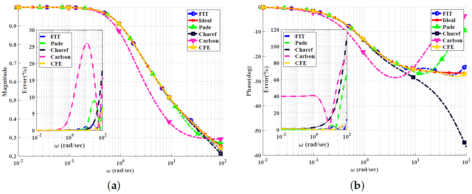
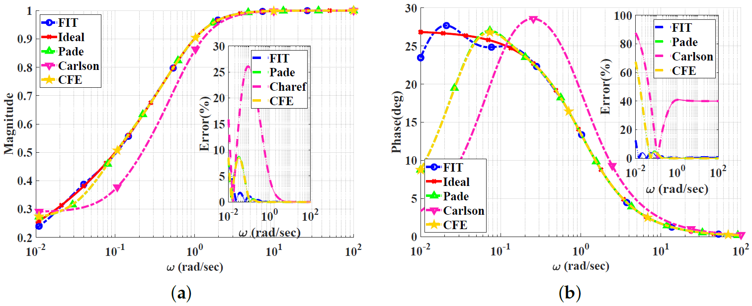
4.1. low-pass power-law Filter

For the pole frequency ${\omega }_0=1$ rad/sec, the transfer function for the low-pass power-law filter is given by Equation (37):

$$H\left(s\right)={\left(\frac{1}{1+s}\right)}^{\alpha }.$$

(37)

Figure 2, Figure 3, Figure 4 and Figure 5 show the magnitude and phase responses and percentage errors of the different approximations for $\alpha =0.3,0.5,0.7,0.9$, respectively.

Table 1. Maximum relative gain percentage errors observed for different orders of the low-pass power-law filter.

Approximation	Error (%)
	$\mathbf{\alpha }$= 0.3	$\mathbf{\alpha }$= 0.5	$\mathbf{\alpha }$= 0.7	$\mathbf{\alpha }$= 0.9
Padé	8	13	10	10
Charef	18	10	2	0.3
Carlson	26	16	80	80
Curve-fitting	2	3	7	7.5
CFE	5	8	5	3

and

Table 2. Maximum relative phase percentage errors observed for different orders of the low-pass power-law filter.

Approximation	Error (%)
	$\mathbf{\alpha }$= 0.3	$\mathbf{\alpha }$= 0.5	$\mathbf{\alpha }$= 0.7	$\mathbf{\alpha }$= 0.9
Padé	62	20	40	19
Charef	80	20	18	3
Carlson	80	20	50	80
Curve-fitting	5	4	8	2
CFE	1	1	3	1

summarize the maximum gain and phase percentage errors observed for different orders.

The CFE and the curve-fitting approximations exhibit minor magnitude and phase percentage errors, both being less than 10%. The Carlson approximation exhibits the most significant percentage errors for $\alpha =0.3,0.7,0.9$. The percentage errors for the Padé approximation start to increase at high frequencies, as demonstrated in Figure 2 for $\alpha =0.3$, the phase percentage error reaching around 62%. The Charef approximation provides a good approximation for $\alpha =0.5,0.7,0.9$ but exhibits a significant phase percentage error for $\alpha =0.3$. From this, we can observe that the Carlson approximation can be used only for $\alpha =0.5$, with maximum relative percentage errors of $16\%$ and $20\%$ for the gain and phase, respectively. The Padé approximation is a good choice for $\alpha =\{0.5,0.9\}$, with maximum relative gain percentage errors of $13\%$ and $10\%$, and phase percentage errors of $20\%$ and $19\%$ The Charef approximation is a perfect choice for $\alpha =0.9$, exhibiting maximum relative gain and phase percentage errors of $0.3\%$ and $3\%$. The curve-fitting approximation is perfect for $\alpha =0.5$, exhibiting maximum relative gain and phase percentage errors of $3\%$ and $4\%$, respectively. The CFE approximation is a perfect choice for $\alpha =0.7$, with maximum relative gain and phase percentage errors of $5\%$ and $3\%$, respectively.

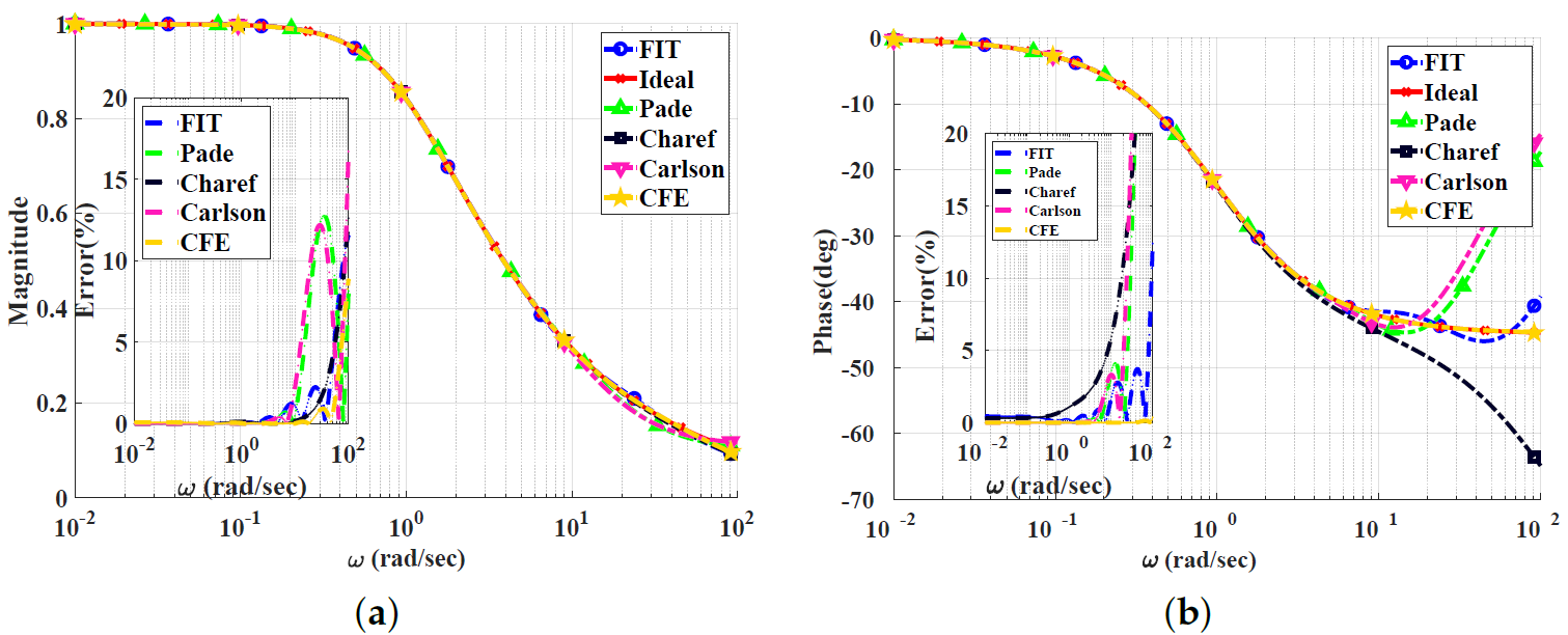
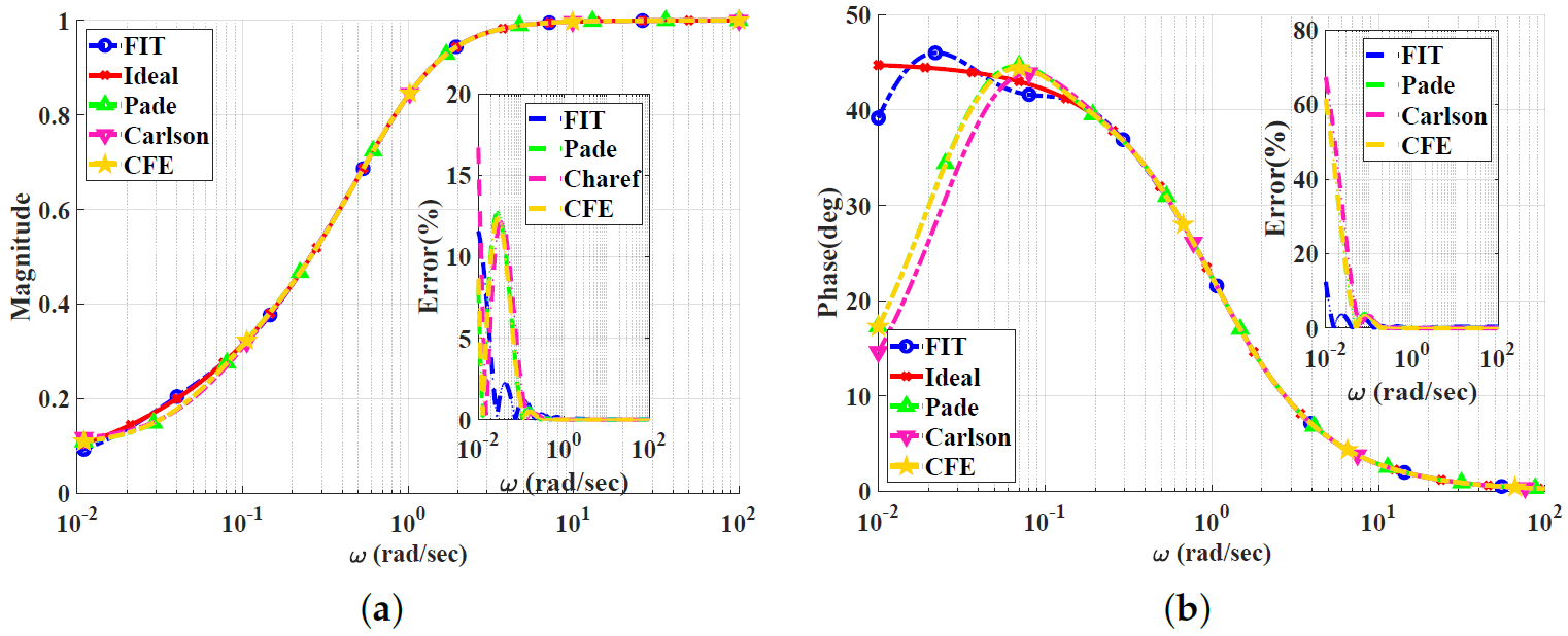
4.2. high-pass power-law Filter

For the pole frequency ${\omega }_0=1$ rad/s, the transfer function for the high-pass power-law filter is given by Equation (38):

$$H\left(s\right)={\left(\frac{s}{1+s}\right)}^{\alpha }.$$

(38)

Figure 6, Figure 7, Figure 8 and Figure 9 show the magnitude and phase responses and percentage errors of the different approximations for $\alpha =0.3,0.5,0.7,0.9$, respectively.

Table 3. Maximum relative gain percentage errors observed for different orders of the high-pass power-law filter.

Approximation	Error (%)
	$\mathbf{\alpha }$= 0.3	$\mathbf{\alpha }$= 0.5	$\mathbf{\alpha }$= 0.7	$\mathbf{\alpha }$= 0.9
Padé	8	14	18	10
Charef	-	-	-	-
Carlson	26	13.5	100	100
Curve-fitting	1	10	18	5
CFE	9	13	18	10

and

Table 4. Maximum relative phase percentage errors observed for different orders of the high-pass power-law filter.

Approximation	Error (%)
	$\mathbf{\alpha }$= 0.3	$\mathbf{\alpha }$= 0.5	$\mathbf{\alpha }$= 0.7	$\mathbf{\alpha }$= 0.9
Padé	60	60	48	19
Charef	-	-	-	-
Carlson	90	63	100	100
Curve-fitting	18	19	8	1
CFE	60	60	48	32

summarize the maximum gain and phase percentage errors observed for different orders. We can see that the curve-fitting approximation exhibits the smallest percentage errors, the CFE and Padé approximations are similar, and the Carlson approximation exhibits large approximation percentage errors, except for $\alpha =0.5$. As a result, the Carlson approximation can be used only for $\alpha =0.5$ and is not preferred, as the other approximations exhibit better percentage errors. Similar to the low-pass power-law filters, the Padé approximation is a good choice for $\alpha =0.9$, with maximum relative gain percentage error of $10\%$, and phase percentage error of $19\%$. The Charef approximation is unsuitable for approximating the high-pass power-law filter, as it is designed to approximate the slope of $-20\alpha$ dB/dec by using zig-zag lines with individual slopes of $-20$ dB/dec and 0 dB/dec. Additionally, the high- and low-frequency properties of the magnitude of the transfer function lead to the lowest and highest singularities of the transfer function approximation being poles. The curve-fitting approximation is a perfect choice for $\alpha =\{0.5,0.9\}$, with maximum relative gain percentage errors of $10\%$ and $5\%$, and phase percentage errors of $19\%$ and $1\%$, respectively. Finally, the CFE approximation is only good for magnitude approximation and does not offer a better choice for any alpha from a phase point of view.

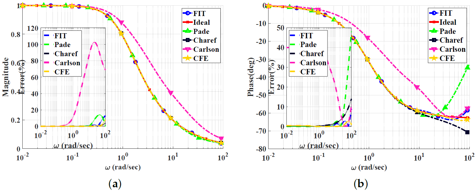
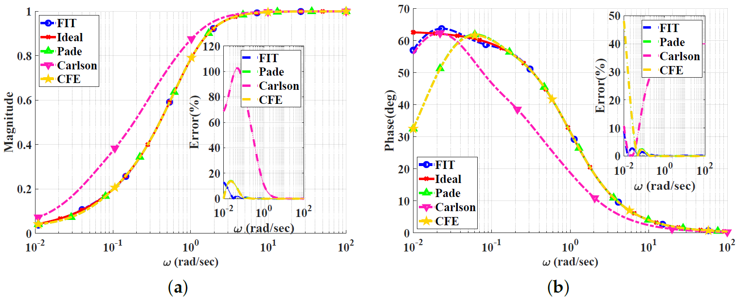
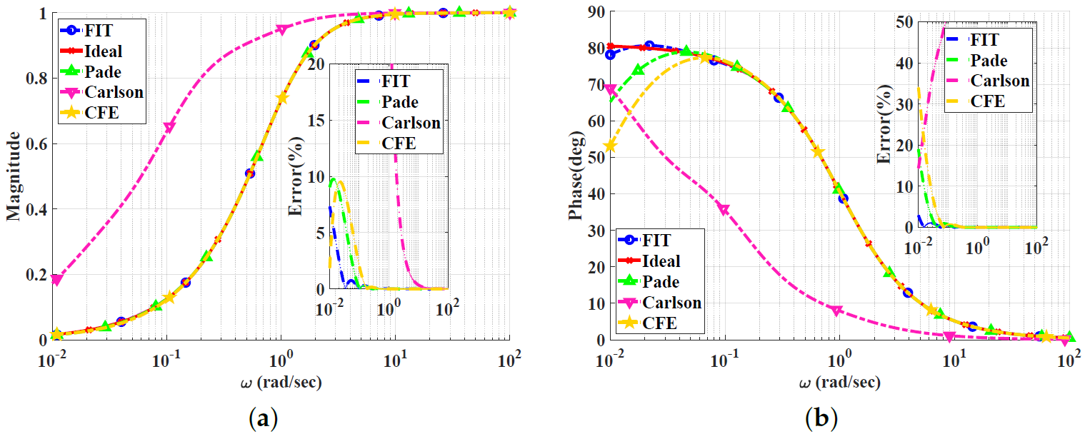
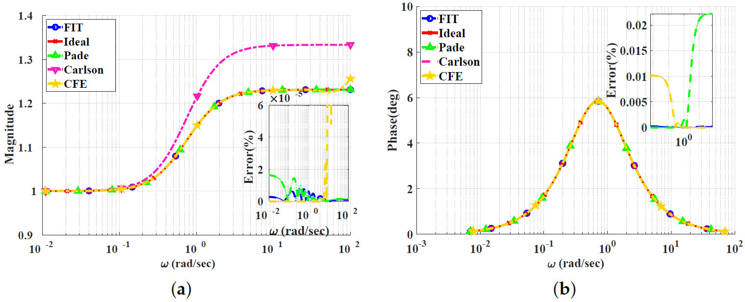
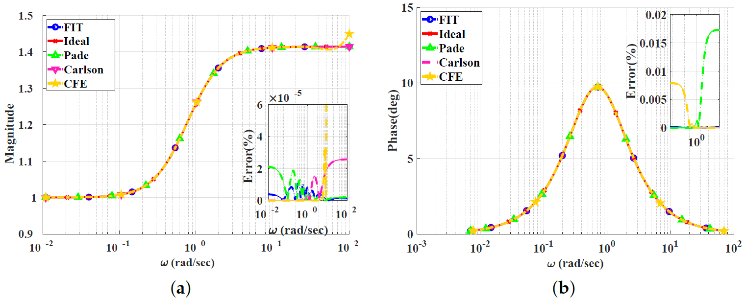
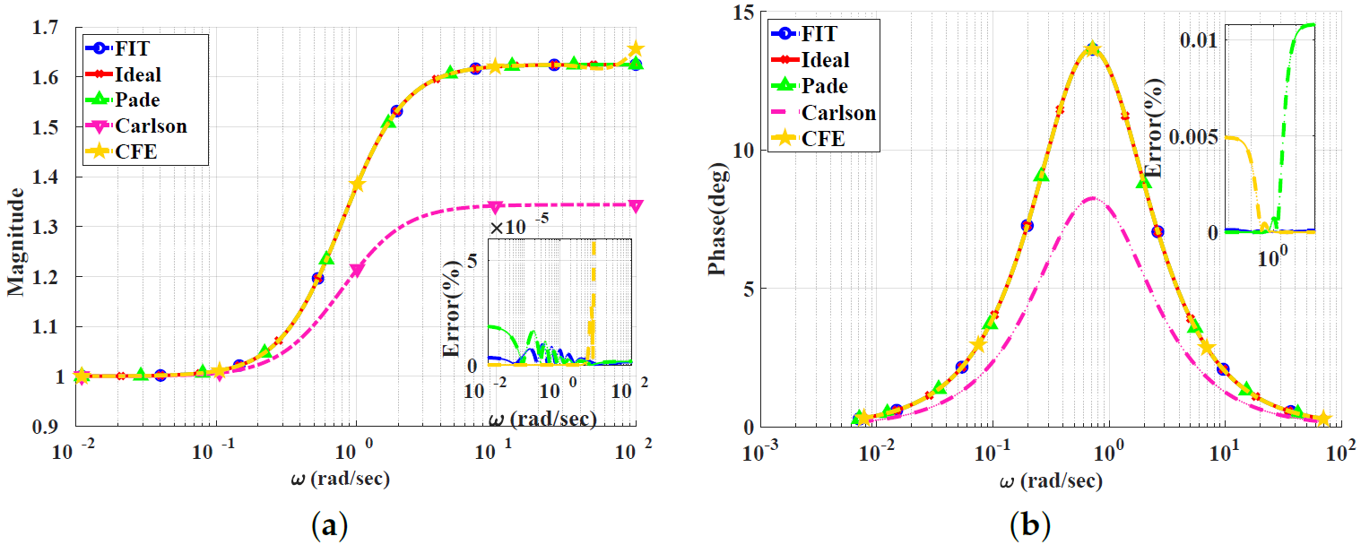
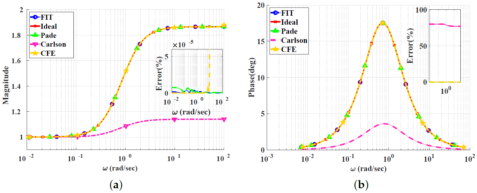
4.3. Power-Law Lead/Lag Compensator

The lead compensator case by substituting in Equation (9) with $K=1$, $x=0.5$, $\tau =2$ s, ${\omega }_m=0.707$ rad/s (the geometric mean of the pole and zero frequencies), and $f_m=0.1125$ Hz, yields:

$$H\left(s\right)={\left(\frac{1+2s}{1+s}\right)}^{\alpha }.$$

(39)

Figure 10, Figure 11, Figure 12 and Figure 13 show the magnitude and phase responses and percentage errors of the different approximations for $\alpha =0.3,0.5,0.7,0.9$, respectively.

Table 5. Maximum relative gain percentage errors observed for different orders of the lead compensator.

Approximation	Error (%)
	$\mathbf{\alpha }$= 0.3	$\mathbf{\alpha }$= 0.5	$\mathbf{\alpha }$= 0.7	$\mathbf{\alpha }$= 0.9
Padé	0.1	0.001	0	0
Carlson	9	0.001	9	50
Curve-fitting	0.1	0	0	0
CFE	0.1	0.001	0.01	0

and

Table 6. Maximum relative phase percentage errors for different orders of the lead compensator.

Approximation	Error (%)
	$\mathbf{\alpha }$= 0.3	$\mathbf{\alpha }$= 0.5	$\mathbf{\alpha }$= 0.7	$\mathbf{\alpha }$= 0.9
Padé	0.03	0.019	0.01	0
Carlson	0.001	0	10	80
Curve-fitting	0	0	0	0
CFE	0.01	0.009	0.005	0

summarize the maximum gain and phase percentage errors observed for different orders. The curve-fitting approximation exhibits the lowest approximation percentage errors, with almost all being zero, followed by the CFE approximation then the Padé approximation. The Carlson approximation exhibits high approximation percentage errors for $\alpha =\{0.7,0.9\}$. As we can see, the Carlson approximation yields better results when used for the lead compensator compared to the filters, exhibiting maximum relative gain percentage errors of $9\%$, $0.001\%$ and phase percentage errors of $0.001\%$, $0\%$ for $\alpha =\{0.3,0.5\}$, respectively. It is not a good choice for $\alpha =0.9$ for phase approximation, with a maximum relative phase percentage error of $80\%$. The Padé approximation exhibits a percentage error of zero for $\alpha =0.9$. The Charef approximation is not used, as discussed in the previous sections. The curve-fitting approximation exhibits percentage errors of zero for $\alpha =\{0.5,0.7,0.9\}$, and the CFE also exhibits a percentage error of zero for $\alpha =0.9$.

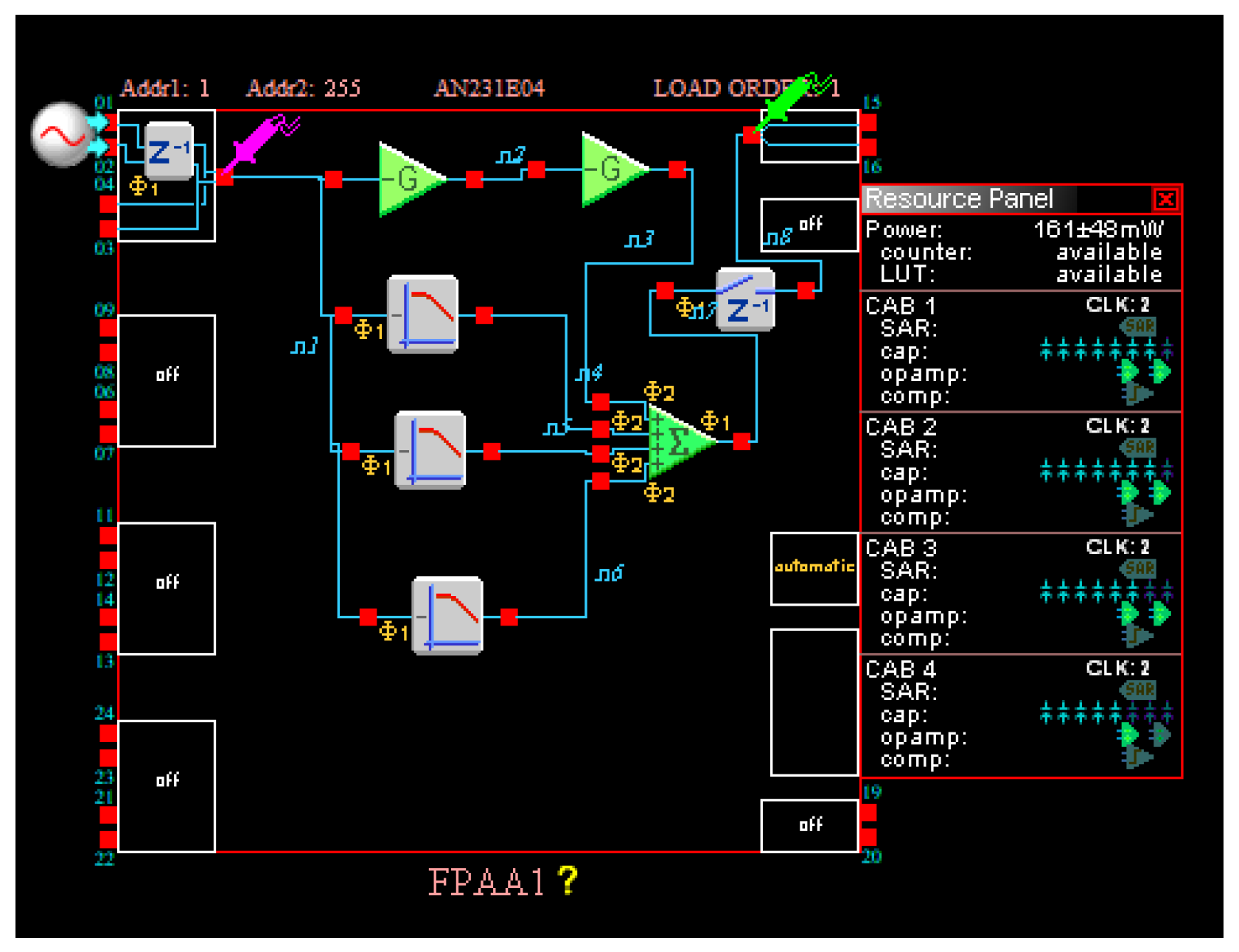
5. FPAA Implementation

Field-programmable analog arrays (FPAAs) are used in analog signal processing, similar to field-programmable gate arrays (FPGAs) in digital signal processing [30]. Operations that can be performed using FPAAs include differentiation, integration, subtraction, summation, division, multiplication, scaling, and filtering [31]. In addition, the low-pass filter, high-pass filter, and lead compensator are implemented using the curve-fitting and CFE techniques, which yield smaller magnitude and phase approximation errors, as discussed in the previous section. The AN231K04 AnadigmApex development board is programmed through the AnadigmDesigner®2 EDA software, version 2.8.0.10 [32].

5.1. Converting the Transfer Functions for Implementation on the FPAA

The rational integer-order transfer functions resulting from the different approximation techniques are converted to partial fraction expansions for implementation on the FPAA using the FPAA configurable analog modules(CAMS), as follows:

$$TF\left(s\right)=\frac{a_3{s}^3+a_2{s}^2+a_{1}s+a_0}{b_3{s}^3+b_2{s}^2+b_{1}s+b_0}$$

(40)

The partial fraction expansion will be in the form:

$$TF\left(s\right)=\frac{k_1}{s+k_1}+\frac{k_2}{s+k_2}+\frac{k_3}{s+k_3}+C.$$

(41)

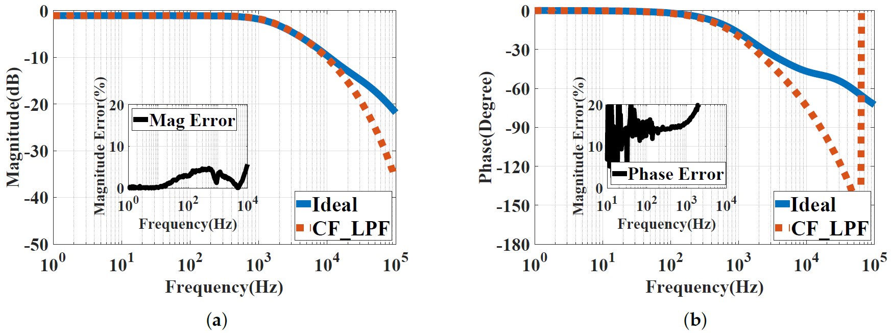
5.2. Curve-Fitting-Based Implementation for low-pass power-law Filters

For the low-pass power-law filter,

$$H\left(s\right)={\left(\frac{1}{1+s}\right)}^{0.5}$$

(42)

The approximated rational integer-order transfer function using curve fitting (fitfrd) is:

$$G_{fitfrd}\left(s\right)=\frac{0.057s^3+7.827s^2+85.52s+140}{s^3+33.77s^2+155.2s+140}.$$

(43)

The partial fraction expansion form is:

$$G_{fitfrd}\left(s\right)=\frac{4.104}{s+28.496}+\frac{1.177}{s+4.066}+\frac{0.616}{s+1.208}+0.057.$$

(44)

Based on the standard Follow-the-Leader-Feedback (FLF) multi-feedback structure, as described by the transfer function [16]:

$$H_{FLF}\left(s\right)=\frac{G_3{s}^3+\frac{G_2}{{\tau }_1}{s}^2+\frac{G_1}{{\tau }_1{\tau }_2}s+\frac{G_0}{{\tau }_1{\tau }_2{\tau }_3}}{s^3+\frac{1}{{\tau }_1}{s}^2+\frac{1}{{\tau }_1{\tau }_2}s+\frac{1}{{\tau }_1{\tau }_2{\tau }_3}},$$

(45)

where ($G_i$) is the gain constant, and (${\tau }_i$) is the time constant. The IFLF topology is commonly used in cases where differential signals are used, whereas parallel filters are preferably used in the case of current-mode signals [16]. The gain factors and time constants, obtained by comparing the coefficients of Equations (43) and (45), are shown in

Table 7. Time constants and scaling factors to transform Equation (44) into the form of Equation (45).

Time Constants			Scaling Factors
${\tau }_1$	${\tau }_2$	${\tau }_3$	$G_0$	$G_1$	$G_2$	$G_3$
0.03	0.218	1.109	1	0.551	0.232	0.057

.

For implementation on an FPAA using the sum of integrators, Equation (44) must be of the form:

$$G\left(s\right)=k_0+\frac{k_1}{1+{\tau }_{1}s}+\frac{k_2}{1+{\tau }_{2}s}+\frac{k_3}{1+{\tau }_{3}s},$$

(46)

where $k_n$ and ${\tau }_n$ represent the gain and time constant of the nth integrator in the FPAA.

Table 8. Values of the scaling factors and time constants for the implemented transfer function presented in Equation (44).

Scaling Factors		Time Constants
Variable	Value	Variable	Value
$k_0$	0.057
$k_1$	0.144	${\tau }_1$	0.035
$k_2$	0.29	${\tau }_2$	0.246
$k_3$	0.509	${\tau }_3$	0.828

summarizes the values of these factors.

The experimental results shown in Figure 14 using the NI ELVIS II show frequency responses within the range of [1, 100k ] Hz of the low-pass power-law filter of ($\alpha =0.5$). The difference in magnitude percentage errors between the ideal response and the approximated curve-fitting FPAA implementation is less than 10%, and it is almost zero at frequencies less than the cut-off frequency, as shown in Figure 14a. The phase percentage error shown in Figure 14b is less than 20% within the frequency band of interest before the attenuation. When comparing the errors observed in the experiment to the theoretical errors in Table 1, we can see a higher percentage of errors in the experiment, caused by the parasitic elements of the NI ELVIS II kit and the FPAA’s internal connections.

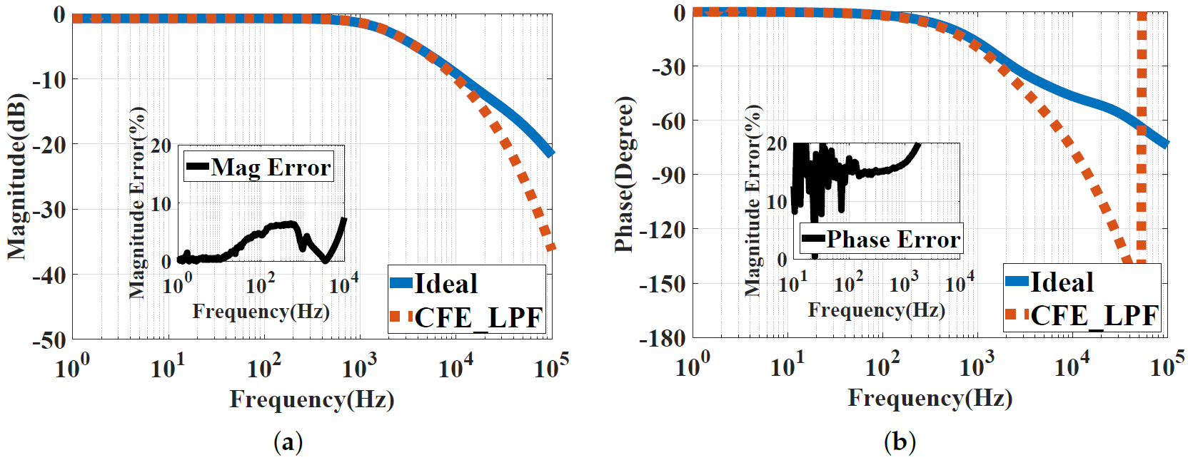
5.3. CFE-Based Implementation for low-pass power-law Filters

The rational transfer function obtained from the CFE approximation for the low-pass power-law filter with $\alpha =0.5$ and $\tau =1$ is:

$$H{\left(s\right)}_{CFE}=\frac{s^3+129s^2+1515s+2899}{17.15s^3+565.8s^2+2932s+2912}.$$

(47)

Using partial fraction expansion, the transfer function of Equation (47) is:

$$H{\left(s\right)}_{PFE}=\frac{3.717}{s+26.862}+\frac{1.145}{s+4.817}+\frac{0.736}{s+1.312}+0.058$$

(48)

So, the implemented transfer function is as follows:

$$H\left(s\right)=\frac{k_1}{{\tau }_{1}s+1}+\frac{k_2}{{\tau }_{2}s+1}+\frac{k_3}{{\tau }_{3}s+1}+k_0.$$

(49)

The values of the scaling factors k and time constants $\tau$ using Equations (48) and (49) are summarized in

Table 9. Values of the scaling factors and time constants for the implemented transfer function presented in Equation (48).

Scaling Factors		Time Constants
Variable	Value	Variable	Value
$k_0$	0.058
$k_1$	0.138	${\tau }_1$	0.037
$k_2$	0.238	${\tau }_2$	0.208
$k_3$	0.561	${\tau }_3$	0.762

.

For the FPAA implementation, the transfer function utilized is in Equation (50),

Table 10. Values of the scaling factors and time constants for the implemented transfer function presented in Equation (49).

Scaling Factors		Time Constants
Variable	Value	Variable	Value
G	0.138	f	4.275
G	0.238	f	0.767
G	0.561	f	0.208

shows the substituted coefficients from Equation (48) [33]:

$$H\left(s\right)=\pm \frac{G\times 2\pi f_0}{s+2\pi f_0}$$

(50)

The experimental results shown in Figure 15 using the NI ELVIS II show the frequency response within the range of [1, 100k] Hz of the CFE approximation for the low-pass power-law filter of $\alpha =0.5$. The difference in the magnitude percentage errors between the ideal response and the approximated curve-fitting FPAA implementation is less than 10%, and it is almost zero at frequencies less than the cut-off frequency, as shown in Figure 15a. The phase percentage error shown in Figure 15b is less than 20% within the frequency band of interest before the attenuation.

5.4. Lead Compensator FPAA Implementation

The curve-fitting approximation’s integer-order transfer function is:

$$H=\frac{1.414s^3+2.9s^2+1.936s+0.421}{s^3+2.301s^2+1.725s+0.421}$$

(51)

and its partial fraction expansion form is:

$$H\left(s\right)=\frac{-0.225}{s+0.97}+\frac{-0.099}{s+0.758}+\frac{-0.03}{s+0.57}+1.41$$

(52)

arranging it in the form:

$$H\left(s\right)=\frac{K_1}{{\tau }_{1}s+1}+\frac{K_2}{{\tau }_{2}s+1}+\frac{K_3}{{\tau }_{3}s+1}+K_0.$$

(53)

$$H=\frac{-0.232}{1.031s+1}+\frac{-0.131}{1.32s+1}+\frac{-0.052}{1.75s+1}+1.41$$

(54)

The curve-fitting FPAA implementation is demonstrated in Figure 16. The reason for cascading two gain stages in the FPAA implementation is to enhance the range of implementable scaling factors [34].

The CFE approximation’s integer-order transfer function is:

$$H=\frac{1.09s^3+2.3s^2+1.57s+0.35}{0.77s^3+1.82s^2+1.4s+0.35}$$

(55)

and its partial fraction expansion form is:

$$H\left(s\right)=\frac{-0.143}{s+1}+\frac{-0.223}{s+0.784}+\frac{0.007}{s+0.58}+1.416$$

(56)

arranging it in the form:

$$H\left(s\right)=\frac{K_1}{{\tau }_{1}s+1}+\frac{K_2}{{\tau }_{2}s+1}+\frac{K_3}{{\tau }_{3}s+1}+K_0.$$

(57)

$$H=\frac{-0.1423}{s+1}+\frac{-0.285}{1.276s+1}+\frac{0.012}{1.724s+1}+1.416$$

(58)

The last equation (transfer function) for the approximated CFE can be realized on the FPAA the same way the approximated curve-fitting one has done.

6. Conclusions

This paper discussed different fractional-order power-law form approximation techniques using MATLAB and implemented an application case study using an FPAA. The design procedure operated in the frequency domain within the range of [${10}^{-2}$, ${10}^2$] rad/s. The fractional-order power-law forms were simulated with orders $\alpha =\{0.3,0.5,0.7,0.9\}$. The performance of the filters was evaluated through simulations and experiments in the cases of the first mother functions of the low- and high-pass filters, and lead compensator. A third-order approximation was utilized, implementing low- and high-pass filters and a lead compensator, with the obtained results showing that accurate operation was achieved. The curve-fitting and CFE approximations exhibited the best performance in our case. However, the Carlson approximation was only good when $\alpha =0.5$ for the low- and high-pass filters. Also, it was good for the lead compensator approximation. On the other hand, the Charef approximation was not compatible with the lead compensator. The accuracy of the Padé approximation highly depended on the center frequency used.

Table 11. Comparison of test cases for power-law filter approximations.

Approximation	Case (1): Denominator $\mathit{H}\left(\mathit{s}\right)=\mathit{k}\times {\left(\frac{1}{1+\mathit{s}}\right)}^{\mathit{\alpha }}$	Case (2): Compensator $\mathit{H}\left(\mathit{s}\right)=\mathit{k}\times {\left(\frac{1+\mathit{Ts}}{1+\mathit{xTs}}\right)}^{\mathit{\alpha }}$
Padé	✓	✓
Charef	✓	X
Carlson	✓	✓
Curve-fitting	✓	✓
CFE	✓	✓

demonstrates which approximation technique is suitable for each power-law filter formula.

The comparative analysis of the different approximations is general and can be applied to all known integer-order filter functions. In addition, all conventional design methods and active elements could be utilized. For example, more robust operational transconductance amplifiers (OTAs) implemented using integrated circuit technology could be utilized. Future research could include employing a more general approximation technique with high accuracy for different power-law form applications. This technique could then be used to implement different applications in controllers for precision mechatronic systems.

References

1. Luo, Y.; Chen, Y. Fractional Order Motion Controls; John Wiley & Sons: Hoboken, NJ, USA, 2012. [Google Scholar]
2. Bošković, M.Č.; Rapaić, M.R.; Šekara, T.B.; Mandić, P.D.; Lazarević, M.P.; Cvetković, B.; Lutovac, B.; Daković, M. On the rational representation of fractional order lead compensator using Padé approximation. In Proceedings of the 2018 7th Mediterranean Conference on Embedded Computing (MECO), Budva, Montenegro, 10–14 June 2018; IEEE: Piscataway, NJ, USA, 2018; pp. 1–4. [Google Scholar]
3. Tsirimokou, G.; Psychalinos, C.; Elwakil, A. Design of CMOS Analog Integrated Fractional-Order Circuits: Applications in Medicine and Biology; Springer International Publishing: Berlin/Heidelberg, Germany, 2017. [Google Scholar]
4. Xue, D. Fractional-Order Control Systems: Fundamentals and Numerical Implementations; Walter de Gruyter GmbH & Co KG: Berlin/Heidelberg, Germany, 2017; Volume 1. [Google Scholar]
5. Kapoulea, S.; Psychalinos, C.; Elwakil, A.S. Versatile Field-Programmable Analog Array Realizations of Power-Law Filters. Electronics 2022, 11, 692. [Google Scholar] [CrossRef]
6. Hamed, E.M.; Said, L.A.; Madian, A.H.; Radwan, A.G. On the approximations of CFOA-based fractional-order inverse filters. Circuits Syst. Signal Process. 2020, 39, 2–29. [Google Scholar] [CrossRef]
7. Monje, C.; Ramos, F.; Feliu, V.; Vinagre, B. Tip position control of a lightweight flexible manipulator using a fractional order controller. IET Control. Theory Appl. 2007, 1, 1451–1460. [Google Scholar] [CrossRef]
8. Dutta, P.; Horn, P. Low-frequency fluctuations in solids: 1 f noise. Rev. Mod. Phys. 1981, 53, 497. [Google Scholar] [CrossRef]
9. Sun, H.H.; Onaral, B. A Unified Approach to Represent Metal Electrode Polarization. IEEE Trans. Biomed. Eng. 1983, BME-30, 399–406. [Google Scholar] [CrossRef] [PubMed]
10. Charef, A.; Sun, H.; Tsao, Y.; Onaral, B. Fractal system as represented by singularity function. IEEE Trans. Autom. Control 1992, 37, 1465–1470. [Google Scholar] [CrossRef]
11. Kapoulea, S.; Tsirimokou, G.; Psychalinos, C.; Elwakil, A.S. Employment of the Padé approximation for implementing fractional-order lead/lag compensators. AEU-Int. J. Electron. Commun. 2020, 120, 153203. [Google Scholar] [CrossRef]
12. Nako, J.; Psychalinos, C.; Elwakil, A.S.; Minaei, S. Non-Integer Order Generalized Filters Designs. IEEE Access 2023, 11, 116846–116859. [Google Scholar] [CrossRef]
13. Sladok, O.; Koton, J.; Kubanek, D.; Dvorak, J.; Psychalinos, C. Pseudo-differential (2+ α)-order Butterworth frequency filter. IEEE Access 2021, 9, 92178–92188. [Google Scholar] [CrossRef]
14. Elwy, O.; Rashad, S.H.; Said, L.A.; Radwan, A.G. Comparison between three approximation methods on oscillator circuits. Microelectron. J. 2018, 81, 162–178. [Google Scholar] [CrossRef]
15. Elwy, O.; AbdelAty, A.M.; Said, L.A.; Madian, A.H.; Radwan, A.G. Two implementations of fractional-order relaxation oscillators. Analog Integr. Circuits Signal Process. 2021, 106, 421–432. [Google Scholar] [CrossRef]
16. Kapoulea, S.; Psychalinos, C.; Elwakil, A.S. Power law filters: A new class of fractional-order filters without a fractional-order Laplacian operator. AEU-Int. J. Electron. Commun. 2021, 129, 153537. [Google Scholar] [CrossRef]
17. Gadallah, S.I.; Ghoneim, M.S.; Elwakil, A.S.; Said, L.A.; Madian, A.H.; Radwan, A.G. Plant Tissue Modelling Using Power-Law Filters. Sensors 2022, 22, 5659. [Google Scholar] [CrossRef] [PubMed]
18. Monje, C.A.; Calderon, A.J.; Vinagre, B.M.; Feliu, V. The fractional order lead compensator. In Proceedings of the Second IEEE International Conference on Computational Cybernetics, Vienna, Austria, 30 August–1 September 2004; IEEE: Piscataway, NJ, USA, 2004; pp. 347–352. [Google Scholar]
19. Dogruer, T.; Tan, N. Lead and lag controller design in fractional-order control systems. Meas. Control 2019, 52, 1017–1028. [Google Scholar] [CrossRef]
20. Kosmas, D.; Schouten, M.; Krijnen, G. Hysteresis Compensation of 3D Printed Sensors by a Power Law Model with Reduced Parameters. In Proceedings of the 2020 IEEE International Conference on Flexible and Printable Sensors and Systems (FLEPS), Manchester, UK, 16–19 August 2020; pp. 1–4. [Google Scholar] [CrossRef]
21. Valério, D.; Da Costa, J.S. Introduction to single-input, single-output fractional control. IET Control Theory Appl. 2011, 5, 1033–1057. [Google Scholar] [CrossRef]
22. Oprzedkiewicz, K.; Mitkowski, W.; Gawin, E. Application of fractional order transfer functions to modeling of high—Order systems. In Proceedings of the 2015 20th International Conference on Methods and Models in Automation and Robotics (MMAR), Miedzyzdroje, Poland, 24–27 August 2015; IEEE: Piscataway, NJ, USA, 2015; pp. 1169–1174. [Google Scholar]
23. Ushakov, P.A.; Maksimov, K.O.; Stoychev, S.V.; Gravshin, V.G.; Kubanek, D.; Koton, J. Synthesis of elements with fractional-order impedance based on homogenous distributed resistive-capacitive structures and genetic algorithm. J. Adv. Res. 2020, 25, 275–283. [Google Scholar] [CrossRef]
24. Tsouvalas, E.; Kapoulea, S.; Psychalinos, C.; Elwakil, A.S.; Jurišić, D. Electronically Controlled Power-Law Filters Realizations. Fractal Fract. 2022, 6, 111. [Google Scholar] [CrossRef]
25. Deniz, F.N.; Alagoz, B.B.; Tan, N.; Atherton, D.P. An integer order approximation method based on stability boundary locus for fractional order derivative/integrator operators. ISA Trans. 2016, 62, 154–163. [Google Scholar] [CrossRef]
26. Andrianov, I.; Shatrov, A. Padé Approximants, Their Properties, and Applications to Hydrodynamic Problems. Symmetry 2021, 13, 1869. [Google Scholar] [CrossRef]
27. Zourmba, K.; Fischer, C.; Gambo, B.; Effa, J.; Mohamadou, A. Fractional integrator circuit unit using Charef approximation method. Int. J. Dyn. Control 2020, 8, 943–951. [Google Scholar] [CrossRef]
28. Das, S.; Pan, I. Basics of fractional order signals and systems. In Fractional Order Signal Processing: Introductory Concepts and Applications; Springer: Berlin/Heidelberg, Germany, 2012; pp. 13–30. [Google Scholar]
29. Chen, Y.; Vinagre, B.M.; Podlubny, I. Continued fraction expansion approaches to discretizing fractional order derivatives—An expository review. Nonlinear Dyn. 2004, 38, 155–170. [Google Scholar] [CrossRef]
30. Kapoulea, S. Interdisciplinary Applications of Fractional-Order Circuits. Ph.D. Thesis, University of Glasgow, Glasgow, Scotland, 2022. [Google Scholar]
31. Azar, A.T.; Vaidyanathan, S.; Ouannas, A. Fractional Order Control and Synchronization of Chaotic Systems; Springer: Cham, Switzerland, 2017; Volume 688. [Google Scholar]
32. Ghali, K.; Dorie, L.; Hammami, O. Dynamically reconfigurable analog circuit design automation through multiobjective optimization and direct execution. In Proceedings of the 2005 International Conference on Microelectronics, Islamabad, Pakistan, 13–15 December 2005; pp. 98–101. [Google Scholar]
33. Bertsias, P.; Kapoulea, S.; Psychalinos, C.; Elwakil, A.S. A collection of interdisciplinary applications of fractional-order circuits. In Fractional Order Systems; Academic Press: Cambridge, MA, USA, 2022; pp. 35–69. [Google Scholar]
34. Nako, J.; Psychalinos, C.; Elwakil, A.S. A 1+ α Order Generalized Butterworth Filter Structure and Its Field Programmable Analog Array Implementation. Electronics 2023, 12, 1225. [Google Scholar] [CrossRef]
Figure 1. Bode plots for the low-pass power-law filter for α = 0.5 using different curve-fitting techniques: (a) Magnitude responses and percentage errors. (b) Phase responses and percentage errors.
Electronics 13 00591 g001
Figure 2. Bode plots for the low-pass power-law filter for α = 0.3 using different approximations: (a) Magnitude responses and percentage errors. (b) Phase responses and percentage errors.
Electronics 13 00591 g002
Figure 3. Bode plots for the low-pass power-law filter for α = 0.5 using different approximations: (a) Magnitude responses and percentage errors. (b) Phase responses and percentage errors.
Electronics 13 00591 g003
Figure 4. Bode plots for the low-pass power-law filter for α = 0.7 using different approximations: (a) Magnitude responses and percentage errors. (b) Phase responses and percentage errors.
Electronics 13 00591 g004
Figure 5. Bode plots for the low-pass power-law filter for α = 0.9 using different approximations: (a) Magnitude responses and percentage errors. (b) Phase responses and percentage errors.
Electronics 13 00591 g005
Figure 6. Bode plots for the high-pass power-law filter for α = 0.3 using different approximations: (a) Magnitude responses and percentage errors. (b) Phase responses and percentage errors.
Electronics 13 00591 g006
Figure 7. Bode plots for the high-pass power-law filter for α = 0.5 using different approximations: (a) Magnitude responses and percentage errors. (b) Phase responses and percentage errors.
Electronics 13 00591 g007
Figure 8. Bode plots for the high-pass power-law filter for α = 0.7 using different approximations: (a) Magnitude responses and percentage errors. (b) Phase responses and percentage errors.
Electronics 13 00591 g008
Figure 9. Bode plots for the high-pass power-law filter for α = 0.9 using different approximations: (a) Magnitude responses and percentage errors. (b) Phase responses and percentage errors.
Electronics 13 00591 g009
Figure 10. Bode plots for the lead compensator for α = 0.3 using different approximation techniques: (a) Magnitude responses and percentage errors. (b) Phase responses and percentage errors.
Electronics 13 00591 g010
Figure 11. Bode plots for the lead compensator for α = 0.5 using different approximation techniques: (a) Magnitude responses and percentage errors. (b) Phase responses and percentage errors.
Electronics 13 00591 g011
Figure 12. Bode plots for the lead compensator for α = 0.7 using different approximation techniques: (a) Magnitude responses and percentage errors. (b) Phase responses and percentage errors.
Electronics 13 00591 g012
Figure 13. Bode plots for the lead compensator for α = 0.9 using different approximation techniques: (a) Magnitude responses and percentage errors. (b) Phase responses and percentage errors.
Electronics 13 00591 g013
Figure 14. Experimental results showing the frequency responses of the curve-fitting approximation for the low-pass power-law filter of α = 0.5 using the NI ELVIS II kit: (a) Magnitude responses. (b) Phase responses.
Electronics 13 00591 g014
Figure 15. Experimental results showing the frequency responses of the CFE approximation for the low-pass power-law filter of α = 0.5 using the NI ELVIS II kit: (a) Magnitude responses. (b) Phase responses.
Electronics 13 00591 g015
Figure 16. AnadigmDesigner®2 EDA software interface for the lead compensator realized using the curve-fitting technique.
Electronics 13 00591 g016