Abstract
This study presents a robust framework designed to address the limitations of passive infrared (PIR) sensors in home-based elderly monitoring, particularly focusing on false detections and sensor blind times, which compromise data accuracy. While PIR sensors are low-cost and privacy-preserving, their inherent inaccuracies hinder their use in reliable monitoring systems. To overcome these challenges, we propose a novel spatiotemporal data cleaning framework that integrates non-deterministic tracking (NDT) and late-binding adjustment (LBA). This framework enhances the quality and accuracy of sensor data by filtering out false positives and omissions through analysis of walking speed and sensor connectivity. Simulations demonstrated significant improvements in movement tracking accuracy, and real-world experiments involving three elderly participants further validated the framework’s practicality. The experiments confirmed that the proposed method can remove errors such as false positives and false negatives from PIR sensors. It can achieve 90% accuracy in tracking the movements of elderly people, highlighting the potential for this framework to be applied in the real world. The key scientific contribution of this research lies in the development of a scalable, non-wearable indoor tracking solution that reduces the need for dense sensor arrays, making it cost-effective and adaptable to existing infrastructure with minimal modifications. This framework contributes to advancing the field of indoor localization and offers a reliable solution for sensor-based monitoring systems, especially in elderly care, addressing the urgent needs of an aging global population.
1. Introduction
The rapid aging of populations is a global concern, as highlighted by the World Health Organization (WHO), which observes that aging is occurring at an unprecedented rate. Between 2015 and 2050, the proportion of people aged 60 and older is projected to nearly double, rising from 12% to 22% [1]. This demographic shift will significantly impact social security systems, including healthcare and long-term care services. While these challenges persist, maintaining a balanced diet and engaging in regular physical activity can help to reduce the need for long-term care. However, a growing number of elderly individuals now live alone [2], making it difficult for distant family members to detect changes in health or emergencies, thereby increasing the demand for remote monitoring systems.
This study aims to develop a framework for an ambient sensing system that continuously monitors the indoor walking speed and distance traveled by elderly individuals without requiring them to wear any devices [3,4,5]. The system infers health status by analyzing changes in these metrics while ensuring privacy [6,7,8]. This is achieved through the use of indoor tracking technology that processes time-series data from motion sensors to monitor movement within a space, such as a home. The study utilizes passive infrared (PIR) sensors, which detect human motion by capturing presence or absence events, thereby minimizing privacy concerns. Additionally, the widespread availability and affordability of commercially produced PIR sensors enable the implementation of a cost-effective and sustainable system. The proposed framework is device-free and non-intrusive, allowing elderly individuals to maintain their daily routines without disruption.
The fundamental principle of spatiotemporal cleaning for PIR sensor data is based on a network topology representing the possible indoor movement paths between sensors. This topology is used to determine which edge is being traversed by the user, thereby generating movement trajectory data based on the network structure. In this topology, the nodes represent PIR sensors and, when two PIR sensors are triggered at different times, their corresponding nodes are activated. The time difference between the two triggered sensors is also used to calculate movement speed. With this approach, it is possible to generate human movement trajectories by placing only a limited number of PIR sensors at key locations, such as doorways or hallways.
Even in the case of false negatives or false positives, the time-series information allows for corrections when the detected movement is deemed implausible based on the network’s constraints. As a result, this process cleans the PIR sensor data, producing a refined dataset with minimal errors, and ensuring that inaccuracies are mitigated to the greatest extent possible. Wu et al. [9] equipped a single sensor module with multiple PIR sensors, enabling false detections from one sensor to be compensated by information from the others. Consequently, determining false detections requires multiple sensors.
Tabbakha et al. [10] proposed an activity recognition system for tracking the daily lives and indoor locations of elderly individuals. This system uses a wearable device integrating an accelerometer and a gyroscope, along with a BLE (Bluetooth Low Energy) scanner, to collect physical activity and location data. By applying machine learning models, specifically Random Forest and SVM (Support Vector Machine), the system achieves recognition accuracies of 95.03% for activities and 86.58% for locations. High-accuracy tracking systems like this predominantly rely on wearable devices. In contrast, our study demonstrates originality by employing a device-free system that does not require wearable devices, utilizing NDT (non-deterministic tracking) and LBA (late-binding adjustment) for accurate monitoring.
Wu et al. [9] demonstrated the feasibility of non-wearable PIR-based indoor localization systems by developing a network of PIR sensors coupled with a microcontroller to track movement across overlapping detection zones. This system highlights how PIR sensors can be used for indoor localization without requiring complex infrastructure; however, their approach primarily relies on the density of sensors, limiting scalability in real-world environments. Similarly, Ngamakeur et al. [11] applied multiple PIR sensors with deep learning models to enhance localization accuracy, achieving a distance error of 0.25 m. While this study pushes the boundaries of accuracy, the reliance on machine learning introduces computational overhead, which may not be suitable for environments like elderly care, where resource limitations are common. Tao et al. [12] proposed a PIR-based system for tracking multiple individuals in an indoor environment with over 90% accuracy. Although these works demonstrate the potential of PIR sensors for indoor tracking, they tend to focus on enhancing sensor accuracy through dense sensor networks or advanced models, which may be challenging to implement in more constrained environments.
Veronese et al. [13] introduced a PIR probability model aimed at balancing cost and reliability by optimizing sensor placement for unobtrusive indoor monitoring. Their model focuses on enhancing the probability of human detection through precise sensor arrangement and interaction, thereby reducing error rates and optimizing system costs. While their approach provides valuable insights into sensor behavior and placement optimization, our research takes a different direction by addressing data accuracy at the processing level rather than focusing solely on sensor deployment.
Instead of optimizing sensor placement, our framework improves data interpretation using non-deterministic tracking (NDT) and late-binding adjustment (LBA). PIR sensors often generate uncertain errors, such as false positives and missed detections, due to ambient temperature fluctuations and indoor obstacles. To effectively address this uncertainty, we employ NDT, which can consider multiple possibilities simultaneously to enhance tracking accuracy, and LBA, which retrospectively identifies the most plausible path among multiple possibilities.
Non-deterministic algorithms tend to impose a high computational load as they maintain and track multiple hypotheses simultaneously. This can be particularly challenging in environments with frequent sensor false detections, as the number of hypotheses may grow continuously, making real-time processing increasingly difficult. Additionally, managing multiple hypotheses concurrently can lead to unnecessary branching, ultimately reducing result accuracy. To mitigate these challenges, our study leverages LBA to eliminate or refine unnecessary hypotheses based on additional data, achieving a balance between accuracy and computational efficiency.
These methods provide real-time flexibility and enable retrospective error correction, ensuring the system remains effective even with sparse sensor configurations. This makes the framework more scalable and adaptable for various indoor environments. In contrast, deterministic algorithms commit each detection to a specific path, increasing the risk of inaccurate estimations when sensor errors or missed detections occur.
Shokrollahi et al. [14] reviewed methodologies for PIR sensor-based occupancy monitoring in smart buildings, emphasizing machine learning for improved detection accuracy. Although this work advances the integration of machine learning in PIR-based systems, our research distinguishes itself by avoiding reliance on computationally intensive techniques. Instead, we leverage more practical, algorithmic approaches, allowing for robust tracking and error correction without the need for high processing power, which is especially relevant in resource-limited environments like elderly care facilities.
Khan et al. [15] investigated a method for mapping long-term occupancy patterns in office spaces using wireless PIR sensors in office buildings. In their study, false positives and false negatives were identified as key issues with PIR sensors. To improve detection accuracy, the sensors were installed under desks to minimize the impact of surrounding human movements and environmental changes, thereby reducing the occurrence of false positives. However, in living spaces for the elderly, it is difficult to install PIR sensors in a manner that blocks the surrounding area and restricts detection to only nearby movements.
Sultanabanu et al. [16] applied PIR sensors in a home security system using Arduino (https://www.arduino.cc, accessed on 25 November 2024), highlighting the practical, real-time detection capabilities of PIR sensors. While their focus is on security, their work reinforces the utility of PIR sensors for cost-effective, real-world applications. Our research extends this practical use by employing more practical methods to address the specific challenges of tracking human movement in care environments, such as handling false positives and negatives, which are critical for effective monitoring.
Masciadri et al. [17] developed a multi-resident number estimation method for smart homes using PIR sensors, demonstrating how PIR sensors can be adapted for more complex use cases like occupancy estimation. However, their focus on occupancy estimation contrasts with our emphasis on continuous movement tracking, where accurate real-time correction of sensor data is necessary to monitor individual movements reliably in environments like elderly care. Narayana et al. [18] proposed a novel localization technique using PIR sensors that enhances tracking precision through advanced signal processing. While their focus is primarily on localization accuracy, our research offers a broader framework that incorporates both real-time tracking and retrospective error correction through NDT and LBA. This ensures that our system can adapt to dynamic environments where movement patterns may be inconsistent, such as in elderly care settings, where individuals may exhibit varied mobility levels throughout the day.
This paper is structured as follows: Section 2 introduces the fundamental concepts of the proposed spatiotemporal cleaning method for PIR sensor data, addressing errors and noise using sensor network topology, movement constraints, and other relevant factors; Section 3 details the system configuration, including the hardware, software, and sensor models used; Section 4 presents the spatiotemporal data cleaning framework developed to enhance tracking accuracy for PIR sensors; Section 5 evaluates the proposed LBIS system through simulations; Section 6 presents the results of real-world experiments conducted with elderly participants; Section 7 discusses the system’s effectiveness; finally, Section 8 concludes with a summary of the findings and future directions.
2. Fundamental Concepts and Proposed Methodology
This section formalizes the sensor log data and spatiotemporal data cleaning process using non-deterministic and late-binding methods designed to address erroneous data when tracking the indoor movements of an elderly individual with Passive Infrared (PIR) sensors. These algorithms account for inherent inaccuracies, such as false positives and missed detections, which are often influenced by sensor positioning, individual movement speeds, and sensor blind time.
2.1. Definitions and Preliminaries
We begin by defining the essential components of the proposed methodology:
- PIR Sensor Network (): A graph where each vertex represents a PIR sensor positioned in the indoor environment and each edge represents a feasible direct line of movement between sensors that an individual may take.
- Detection Log (): A sequence of tuples where represents the sensor activated and is the timestamp when sensor was triggered.
- Activation Path of PIR sensors: A sequence of sensors such that, for each consecutive pair, there exists an edge, representing a possible movement path of a user through the PIR sensors to .
- Simulated User Trajectory Data from :
- ○
- Sensor Positions: Let and represent the spatial positions of the two PIR sensors, which are physically fixed within the indoor space.
- ○
- Activation Timing: Let and be the respective timestamps when sensors and are activated.
- Definition of User Presence Points: The user’s presence point at any given time between two sensor activations can be defined based on a linear interpolation between the positions of the two sensors, using the sampling rate as follows:where is the linear interpolation factor that represents the proportion of time elapsed between two activations.
Metrics:
- ○
- Hop Count Function: The hop count between two sensors and , denoted , calculates the minimum number of edges in the shortest path between them in the graph .
- ○
- Distance Function: The physical distance between two sensors and , denoted , is determined by their spatial positions and the setup during sensor installation.
- ○
- Speed Calculation: The walking speed between two detections and , is calculated as
This equation determines the speed based on the physical distance between the sensors and the time elapsed between the two detections.
2.2. False Positives and False Negatives
To accurately define the terms False Positive (FP) and False Negative (FN), we use the following criteria:
- False Positive (FP): A detection by the PIR sensor that does not correspond to actual human movement.
- ○
- Definition: For a detection event , it is considered a false positive if the sensor is activated but no movement is detected by any adjacent sensors within a specific time threshold .
- ○
- Condition: is activated and , if , then is not activated.
Here, denotes the set of sensors adjacent to . This condition ensures that no adjacent sensor detects the movement within the time window , confirming a false positive detection.
- False Negative (): A missed detection where the PIR sensor fails to detect actual movement.
- ○
- Definition: For a sequence of detections and , a false negative occurs if the subject moves between and but no intermediate detections are recorded by sensors located along the path between these two sensors.
- ○
- Condition: is activated, is activated and such that is not activated within []. Here, represents the set of sensors located along the direct movement path between and . A false negative is detected when at least one intermediate sensor is expected to detect the movement but fails to activate during the subject’s movement between and .
2.3. Subject Movement Modes: ‘Moving’ and ‘Staying’
To accurately model the subject’s state, we define three modes of movement based on the time duration and speed between consecutive sensor activations.
- : The subject is detected transitioning between sensors without significant pauses.
- ○
- Condition: , where is the minimum threshold for movement speed, ensuring the subject is actively transitioning between sensors. This mode is triggered when the subject’s movement speed exceeds , indicating continuous movement.
- : The subject remains near a sensor for an extended period, indicating a pause or rest.
- ○
- Condition: where is a time threshold indicating how long the subject remains near the sensor and the speed between the two activations is close to zero. This mode is used when the subject lingers or rests near a sensor for a significant period.
2.4. Integration of Non-Deterministic Tracking and Late-Binding Adjustment for Path Monitoring
In indoor movement tracking using Passive Infrared (PIR) sensors, handling sensor inaccuracies is crucial due to the frequent occurrence of false positives and false negatives. To effectively mitigate these errors, we propose an integrated approach that adapts two complementary algorithms: non-deterministic tracking (NDT) [19,20] and late-binding adjustment (LBA) [21,22]. These algorithms work in tandem, with NDT generating multiple hypotheses for potential movement paths in real-time, and LBA refining and correcting these paths based on later sensor data.
The use of NDT allows the system to explore all possible movement paths without immediately committing to a single interpretation. This flexibility is essential in real-time environments where decisions must be made under uncertainty. LBA, on the other hand, plays a corrective role, adjusting earlier interpretations once additional data become available, ensuring that the final movement paths are as accurate as possible.
The necessity of both NDT and LBA arises from the nature of indoor tracking systems. NDT provides the initial flexibility to hypothesize movement patterns, while LBA ensures robustness by revisiting and refining these hypotheses. Together, they form a dynamic and adaptive framework that consistently corrects errors, such as false positives and false negatives, more effectively through their complementary use.
2.5. Path Tracking Using Non-Deterministic Tracking (NDT)
The non-deterministic tracking [18,19] explores all potential paths through the sensor network without committing to a single path immediately. It retains multiple hypotheses regarding the subject’s movement, which are validated or invalidated as more data become available. The core steps of NDT are as follows:
- (1)
- Initialization: Begin with the initial detection log ().
- (2)
- Path Exploration: For each initial detection , evaluate all subsequent detections where .
- (3)
- Feasibility Check:
- ○
- Calculate the hop count Hop and .
- ○
- Retain the path if it satisfies the following conditions:
- ■
- Hop count.
- ■
- Speed threshold
(e.g., ).
- (4)
- False Positive Check: If the conditions are not met and no adjacent sensors detect movement, mark the detection as a false positive.
- (5)
- Mode Identification: Classify movement as ‘Moving‘ if the speed exceeds a threshold, or ‘Staying‘ if the time between activations is long and the speed is near zero.
- (6)
- Branching: Generate multiple branches of the detection log, each representing a different possible correction, with the movement mode labeled for each path.
2.6. Path Tracking Using Late-Binding Adjustment (LBA)
Late-binding adjustment (LBA) [21,22] complements non-deterministic tracking (NDT) by retrospectively correcting movement paths based on updated sensor data. While NDT generates hypotheses in real-time, LBA revisits earlier decisions to refine or correct errors, thereby improving the accuracy of the overall tracking system. The following steps outline the core process of LBA:
- (1)
- Initial Log Processing: Begin by creating a copy of the detection log , where each detection is assigned an initial state.
- (2)
- Detection Iteration: For each detection event , evaluate all subsequent detection events within the log.
- (3)
- Contradiction Identification:
- ○
- Calculate the speed () and the hop count (=Hop) between each detection pair .
- ○
- If the calculated speed exceeds realistic thresholds or if the hop count is abnormally high, mark the initial detection as potentially erroneous.
- ○
- Additionally, check for false negatives by identifying missing intermediate detections expected between and .
- (4)
- State Adjustment:
- ○
- Adjust the log based on the last confirmed correct detection, modifying states and timestamps for detections from to .
- ○
- Label ‘Staying‘ if the subject stayed near a sensor for an extended period without moving.
- ○
- Update false positives if no corresponding movement is confirmed by adjacent sensors.
Algorithm 1 shows the pseudocode of the data cleaning algorithm that integrates NDT and LBA, as proposed in this study.
| Algorithm 1: The data cleaning algorithm that integrates NDT and LBA |
| Input: DetectionLog DL, SensorGraph G(V, E), TimeThreshold , HopThreshold Hop_Max Input: Speed Threshold Speed_Max Output: RefinedPath RP 1 Initialize HypothesesList 2 For each detection event in DL 3 a. Create initial path ] 4 b. Add P to H 5 For each hypothesis P in H: 6 a. While there are subsequent detections : 7 i. If AND : 8 Append to P 9 ii. Else If no valid adjacent sensor : 10 Mark as False Positive (FP) 11 Break 12 Apply Late Binding Adjustment (LBA) to refine hypotheses in H: 13 a. For each hypothesis P in H: 14 i. Backtrack through P to correct inconsistencies 15 ii. If a detection is invalid: 16 Remove as FP or interpolate as FN 17 iii. Optimize path based on updated data 18 Consolidate valid hypotheses to form RefinedPath RP 19 Return RP |
3. Background and Experimental System: Hardware, Software, and Field Configuration
This study’s system builds on our previous work [23]. Figure 1 shows a smart home for the elderly, with PIR sensors installed on the ceilings in frequently visited areas. The known sensor locations allow for precise distance calculations and synchronized sensors enable the tracking of walking speed and movement. These data are shared with family, caregivers, and healthcare providers to support the early detection of changes in physical activity for improved health monitoring. However, in environments where the user is not living alone, the system may collect data from other individuals, limiting its effectiveness under specific conditions. Additionally, while the system can calculate changes in walking speed, its accuracy is limited unless the user walks consistently at the same speed.
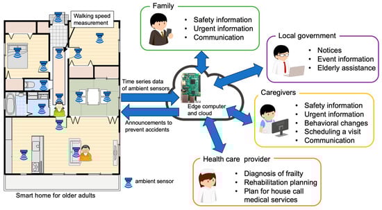
Figure 1.
Smart home setup for elderly residents showing sensor placements for movement detection.
3.1. Detection Range and Error Reduction in Passive Infrared (PIR) Sensors
This study uses the SB612B PIR sensor (Nanyang Senba Optical & Electronics Co. Ltd., Shenzhen, China), which converts infrared radiation into an electrical signal [24,25]. This sensor is mass-produced and easily available at the low price of 4 USD. Table 1 shows the SB612B specifications.

Table 1.
Specifications of the PIR sensor (SB612B).
A PIR sensor module is mounted on the ceiling at 3 m high. As depicted in Figure 2a, the detection range of the PIR sensor , defined by in the horizontal direction, and in the height of the sensor, is calculated using Formula (1). This formula determines the detection diameter of the :
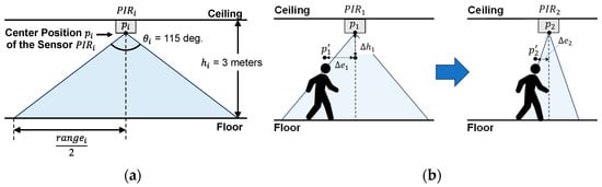
Figure 2.
PIR sensor FOV and detection range. (a) Side view. (b) Detection error: , where is detected, is actual, and is the error. Narrowing the range reduces error, bringing close to .
The detection location of the PIR sensor includes random errors. As illustrated in Figure 2b, the coordinates of the incorporate an independent random variable and is detected at . Conversely, narrowing the sensor’s detection range reduces the error , as shown on the right side of Figure 2b, improving the accuracy of the detected location. Thus, a wide detection range increases error and reduces accuracy in walking speed measurements. Covering the sensor with aluminum tape, which blocks infrared rays, can limit the detection range and reduce these errors.
Two potential concerns arise when covering PIR sensors with aluminum foil [13]. The first is whether reducing the detection range might prevent full coverage of the target space; the second is whether this could impact the detection dynamics, particularly for fast-moving subjects. Our system is designed to track movement trajectories through specific gateway and stay zones rather than providing full area coverage. As long as accurate detection occurs within these zones, there are no issues in generating movement trajectories. While it is true that PIR sensors may fail to detect subjects moving at speeds exceeding two meters per second, this does not happen consistently. If movement is detected by any of the sensors along the path, the movement trajectory can be reconstructed using late-binding adjustment, which mitigates any significant issues [21]. Additionally, since the target users are elderly individuals, high-speed movement within the home environment was rarely observed.
3.1.1. Limitation of the PIR Sensor’s Detection Range
To reduce the PIR sensor’s detection range, its Fresnel lens was partially covered with aluminum tape, leaving about 5 mm exposed around the center, as shown in Figure 3a. The sensor was mounted on the ceiling to measure its detection range, and response points were recorded from eight directions, as illustrated in Figure 3b. For each direction, 10 measurements were taken, and the average of these determined the detection range for that direction. The results showed a detection angle of approximately 21.3 degrees and an average range of 1.13 m. This description is based on the methodology from our previous work [23], which explored the basic detection capabilities of the PIR sensor. We reference these findings as the foundation for this study.
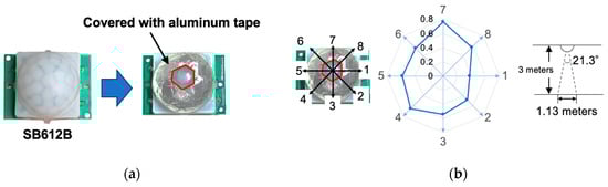
Figure 3.
Measurements of PIR sensor range. (a) The Fresnel lens was partially covered with aluminum tape, leaving 5 mm exposed. (b) Detection range was averaged from 10 measurements per direction.
While the sensor did not produce a symmetric geometry area, as seen in Figure 3b, this lack of symmetry did not significantly affect its performance in detecting human movement. Our experimental results indicate that, even without a perfectly symmetrical detection range, the sensor can still reliably detect the presence of humans, which is the primary objective of this study. The approximate detection range was sufficient for our purposes, and any deviation from perfect symmetry did not hinder the system’s ability to gather accurate movement data. Additionally, we have verified through real-world experiments that the PIR sensor data used for detecting human movement can be collected reliably without issues, despite the irregularities in the detection area. These findings demonstrate that the sensor’s performance remains adequate for our application, even with a reduced detection range.
By narrowing the detection range of PIR sensors, the accuracy of detected locations can be improved; however, this adjustment also increases blind spots and reduces the overall detection area. As a result, detecting human presence throughout all indoor areas becomes unfeasible. Nevertheless, the primary objective of this study is not to monitor every location but to automatically generate human movement trajectories by detecting individuals at key passage points. To achieve this, the detection range of the PIR sensors has been configured to ensure reliable detection in critical areas such as hallways. The sensors have also been strategically positioned to support this goal. Therefore, we do not anticipate any degradation in system performance due to obstacles or other environmental factors.
3.1.2. Construction of PIR Sensors Module
The PIR sensors module employed in this study, previously developed in our work [23], includes a PIR sensor and an ESP8266 microcontroller with wireless capabilities from Espressif Inc. (Shanghai, China). The connection diagram and the module’s appearance are displayed in Figure 4. Assembly of this sensor module involves connecting the PIR sensor to the ESP8266 using power and signal wires, requiring basic technical knowledge, programming, and wiring of the components.
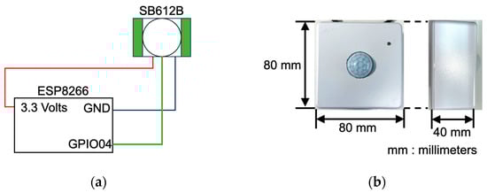
Figure 4.
PIR sensor module. (a) Wiring diagram of the electronic. (b) Compact module appearance.
The PIR sensor outputs a HIGH (3.3 volts) when detecting human motion and maintains this state during the blocking period. Afterward, it switches to LOW (0 volts) if no movement is detected. The ESP8266 monitors the GPIO interface connected to the PIR sensor and detects state changes (from OFF to ON and back to OFF after the blocking time). Upon detecting a change, the ESP8266 uses the MQTT protocol to wirelessly transmit data including time, sensor id, and status (ON or OFF) to an edge computer (Raspberry Pi 4).
3.2. Modeling and Evaluation of PIR Sensor-Based Walking Speed and Movement Tracking in Elderly Environments
The measurement of walking speed was based on the time taken to pass between two designated points. This was assessed using three different methods: manual timing with a stopwatch; laser-based measurements utilizing LiDAR sensors to record the time taken to cross the emitted laser beams; and time measurements from PIR sensors installed at the two points. The comparison of these methods demonstrated that the time intervals measured by the manual stopwatch, LiDAR sensor, and PIR sensor were closely aligned, further validating the accuracy of the PIR sensor module. These experiments provide a comprehensive evaluation of the PIR sensor’s performance, supporting its use in human motion detection and speed measurement [23].
In this study, the PIR sensor modules are integrated into an edge computing system using Raspberry Pi 4 devices. While the Network Time Protocol (NTP) servers are run on a separate PC and not integrated into the edge computers, the PIR sensor modules themselves do not require an Internet connection. By maintaining a connection with the NTP servers, the system ensures accurate time synchronization, providing high-precision clocks for the sensor modules. This setup enhances the temporal quality of the spatiotemporal sensor data.
A key feature of our experimental system is that, even when data from multiple PIR sensor modules is collected and aggregated in a data repository server, there is no time discrepancy between the timestamps of different PIR sensors. This ensures the proper integration of PIR sensor data into a unified spatiotemporal sensor data repository. The experiments were conducted under this system configuration to validate the accuracy of both time and location measurements for indoor walking speed and the movement tracking of elderly individuals.
3.2.1. Modeling of Sensor States and Transfers Between Sensors
A PIR sensor has three states illustrated in Figure 5a: (1) ‘Not Detect’, where the subject is outside the detection area; (2) ‘Detect’, where the subject has entered the detection area; and (3) ‘Blocking Time’, where the PIR sensor remains unresponsive for a set period after detection. During the blocking time, the subject is temporarily undetectable.
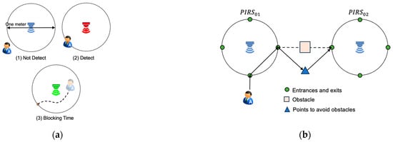
Figure 5.
Sensor state modeling. (a) States include ‘Not Detect’, ‘Detect’, and ‘Blocking Time’ based on subject distance. (b) Model shows movement from to , with trajectories adjusted for obstacles.
Movement between sensors is analyzed using time series data from the sensors, as depicted in Figure 5b. In this model, the subject moves from to . Entrances and exits at PIR sensors are vertically and horizontally aligned, with trajectories connecting them. If obstacle like furniture blocks the path, an intermediate point is added to create a detour.
3.2.2. Sensor Time Series Data
When the sensor detects human motion, it sends the date and time of detection, sensor ID, and status to the edge computer in JSON format. Below is an example of the transmitted data:
- {‘DateTime’: ‘2024/05/01 16:37:18.900000’, ‘EpochTime’: ‘1714549038.900’, ‘ID’:’ PIRS01’, ‘Status’: ‘ON’}
The edge computer collects data from each PIR sensor (PIRS) unit upon state changes, as shown in Figure 6a. These data correspond to those described in Section 3.1.2, transmitted from the sensor module. The edge computer then compiles this into a state change table (Figure 6b) using the collected time series data. If no new data are received, the previous state is maintained, indicating no change. The times in the table are recorded in 0.1-s increments, with t = 0 marking the start of measurement. The interval when the PIR sensor is ON and then turns OFF is known as ‘Blocking Time’, during which the detection of subjects is not possible.
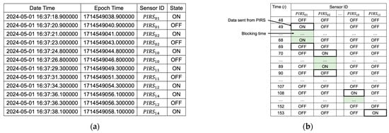
Figure 6.
PIR sensors to edge computer. (a) Sends timestamp, ID, and state change. (b) Edge computer logs state changes. Bold frames show data, green marks blocking time, units in 0.1 s.
3.2.3. Elderly Housing Model and Sensor Placement
Figure 7 illustrates a model of an elderly person’s home used to evaluate the proposed method. PIR sensor units are installed along frequently used pathways in common areas such as kitchens, living rooms, and bathrooms, at room entrances where paths diverge, and at specific locations like beds. In this setup, 14 PIR sensor units are strategically placed within a room measuring 16.25 m by 6.5 m.
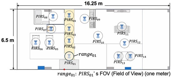
Figure 7.
PIR sensor placement in elderly home. Sensors positioned along movement paths, in kitchens, living rooms, bathrooms, room entrances, and near beds.
Figure 8 demonstrates tracking from the time series data of the PIR sensor using a naive method. In Figure 8a, the method tracks only the time and location when the sensor switches from OFF to ON, assuming the subject remains at the previous location until the next detection occurs. This method does not account for actual movement between detection points, which complicates the understanding of the movement trajectory. Figure 8b improves the visualization by estimating and plotting the subject’s location every 0.1-salong the predefined network topology. The movement is represented as following the shortest path between two PIR sensor units based on the walking speed measured between these sensors. However, movements that deviate from this predefined topology cannot be captured with fine detail.
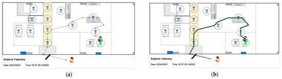
Figure 8.
Naive tracking. (a) Logs PIRS state changes, skipping movement points. (b) Calculates speed between OBAS units, estimating positions every 0.1 s, with path adjustments for obstacles.
4. Implementation of Spatiotemporal Data Cleaning Method for PIR Sensor Data
We introduce LBIS, a late-binding system for correcting inaccurate detections in sensor data, designed to enhance the accuracy of tracking data from PIR sensors. Accurately tracking the indoor movements of elderly individuals and obtaining their trajectories from PIR sensor time series data requires addressing issues like false positives and detection omissions, which are caused by blocking time. This section outlines a method to filter these errors.
4.1. Data Cleaning Method Using Network Topology and Subjects’ Walking Speed
The proposed method filters errors using the PIR sensor network topology and the walking speed between PIR sensor units. The room layout and PIR sensor placement determine the detection sequence during a subject’s movement, enabling the creation of a network topology for the PIR sensor system. For example, as shown in Figure 9a, Subject A entering the room must pass through to reach by the bed, as illustrated in Figure 9b. Upon installation, the exact positions of the PIR sensors are measured, ensuring known distances between units. Each PIR sensor is time-synchronized with the edge computer, allowing precise measurement of transit times and the calculation of walking speeds based on these distances.
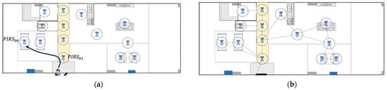
Figure 9.
Example network topology consisting of the indoor layout and placement of PIR sensor (PIRS) units. (a) Subject A at the entrance must pass through to reach the bed where is located. (b) PIRS network topology generated from the connection relationships between each PIRS unit.
In normal tracking, movement between adjacent PIR sensor units represents one hop in the PIR sensor network topology. If a subject moves during the blocking time, resulting in false positives or backtracking, the detection might be missed. Therefore, movements within two hops are considered possible and evaluated based on walking speed. Movements exceeding two hops are deemed false detections.
Previous research has reported an average outdoor walking speed of 1.16 m per second for adults in their 60 s [26], with maximum speeds ranging from 1.4 to 2.2 m per second [27]. However, acknowledging that indoor walking speeds for elderly individuals are typically lower, this study uses a threshold of 2.0 m per second specifically for identifying false positives from PIR sensor detections. Movements detected at speeds exceeding this threshold are unlikely to be genuine and are therefore classified as errors.
Figure 10 illustrates a specific example. In Figure 10a, registers a false positive (t = 60) while the subject moves from to . The corresponding PIR sensor state change table is shown in Figure 10b. In the proposed method, at t = 60, when is detected, the subject was last seen by at t = 50. Since there are three hops from to , it is identified as a false positive. Figure 10c shows a case where the subject passes during a PIR sensor blocking time. The subject is detected by at t = 60, at t = 70, then turns back and is detected by at t = 79 during the blocking time of .The state change table for this scenario is shown in Figure 10d. The subject’s movement appears in the order of , , and , indicating a path via . A pseudo ‘OFF’ is inserted during the blocking time of to generate a backtracking route. Even if the hop count is satisfied, exceeding the speed threshold between PIR sensor units flags it as a false positive.
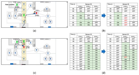
Figure 10.
Cases of PIRS false positives and missed detections. (a) False positive detection at . (b) Route correction by removing false positive. (c) Missed detection during PIRS blocking time. (d) Detection leakage and backtracking route creation.
Suppose that subject is detected by at time and by at time . The function determines the number of hops between and in the network topology, while calculates the distance between them. A decision is then made based on the number of hops and the walking speed between the PIR sensor units, as shown in the following formula:
When Formula (4) is not satisfied, the detection by is considered a false positive. If a false positive is identified, the state change table is updated to adjusts the detected time and blocking time from ‘ON’ to ‘OFF’.
4.2. Implementing Late Binding to Refine Trajectory Data Corrections
In data cleaning using the PIRS (PIR sensor) network topology and walking speed, simply counting hops and measuring speed are insufficient for accurately identifying simultaneous PIRS reactions near a subject, including false positives (Figure 11a). Therefore, when multiple PIRS units simultaneously detect a subject, the unit most likely involved is initially identified. If a subsequent detection occurs at only one unit, the system retroactively corrects the record, assuming the subject moved to that specific unit (Figure 11b).
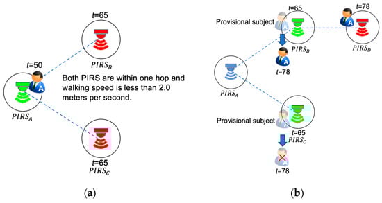
Figure 11.
Late-binding method for correcting log data. (a) Ambiguous movement detection between adjacent PIRS units. (b) Retroactive correction of subject movement based on subsequent detections.
Figure 12 illustrates a specific example. In Figure 12a, the subject passes through at t = 40, at t = 58, and is detected by at t = 77. At t = 58, is also detected, creating ambiguity about whether the movement was from to or . As shown in Figure 12b, the state change table is expanded to include data (time and state), maintaining a record of each state change at every time point. Initially, all states are ‘OFF’. When detects the subject (A) at t = 40, the status changes to ‘ON’ and is labeled as ‘A’. After t = 41, it is marked as ‘A?’ to indicate uncertainly due to blocking time, as it is unclear if the subject remains there.
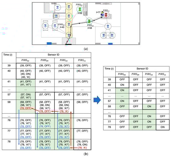
Figure 12.
Late-binding method using a state change table. (a) Ambiguous movement detection between PIRS units. (b) Retroactive correction of subject movement based on later detection.
At t = 58, and are detected simultaneously, leading to their provisional labeling as (58, ‘A?’) due to inestimable movement. At t = 78, only is detected, marked as (78, ‘A’). The provisional detection at , adjacent to , is then assessed for feasibility based on the number of hops and walking speed. If movement from to is feasible, the time at is retroactively adjusted to t = 78, and the provisional (58, ‘A?’) is finalized as (78, ‘A’). This adjustment reflects the finalization of the data at t = 78 and modified accordingly.
Since detected the subject at t = 58, is identified as a false positive and is set to ‘OFF’ at t = 78 to eliminate the error. Similarly, since no subject is detected at , it is also set to ‘OFF’ at t = 78. Using the state change table and referring to the last detected subject from the state change history table as ‘ON’, the correct routes—, , and —are identified, as illustrated on the right in Figure 12b.
5. Evaluation of Spatiotemporal Cleaning of PIR Sensor Data by Simulation
To evaluate the proposed method, we will conduct a simulation before testing with actual equipment. We developed the following three types of software systems from scratch for this purpose:
- (1)
- Integrated Simulation Data Generator (ISDG), which creates PIR sensor data reflecting the subject’s movements within rooms. To evaluate the proposed method, it is possible to introduce various error patterns, such as false positives and missed detections, which are difficult to replicate in real-world experiments.
- (2)
- LBIS data cleaning filter, which remove false positives and other irrelevant information from PIRS time series data produced by the ISDG. Implements LBIS in software to perform data cleaning on sensor data containing errors. This process is also used in real-world experiments.
- (3)
- SensorPathFinder, which visualizes the data cleaned by the LBIS. To evaluate the data before and after the data cleaning process, the tracking results are visualized.
Figure 13 illustrates the simulation evaluation flow. In this phase, the LBIS filter is assessed using simulation data generated by the ISDG, without testing on the actual devices.
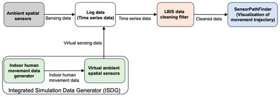
Figure 13.
Data flow diagram of the LBIS data cleaning algorithm evaluation process.
5.1. Integrated Simulation Data Generator (ISDG)
This simulator, ISDG, generates artificial trajectory data by simulating human movement within rooms. Users can draw a polygonal line to represent trajectories using a pointing device such as a mouse and set virtual PIRS locations. The simulator can also generate detection data for two virtual subjects moving simultaneously within virtual rooms. Figure 14 shows a screenshot of the ISDG user interface, developed in Python.
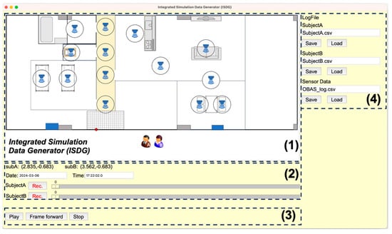
Figure 14.
Integrated Simulation Data Generator (ISDG) interface for generating PIRS detection data based on subject movement.
In area (1) of Figure 14, the indoor movement of a subject is simulated by dragging the subject’s icon with the mouse. In area (2), the subject’s movement is recorded by pressing the ‘Rec.’ button. Once recorded, pressing the ‘Play’ button in area (3) generates the PIR sensor detection data corresponding to the subject’s movement. The resulting time series data of the subject’s movements and PIRS detections can be saved to a text file in area (4).
Figure 15a displays the generated tracking data for a subject, including sequence number, date and time, pixel coordinates, and physical coordinates. Figure 15b shows the detection data from PIRS units, which includes the date, epoch time, sensor ID, and status (‘ON’ or ‘OFF’), mirroring the data detected by physical PIRS devices. Figure 16 presents an example of data generation.
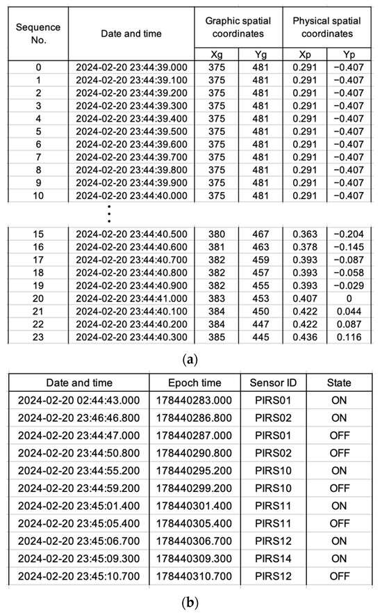
Figure 15.
ISDG data. (a) Records coordinates every 0.1 s with timestamp. (b) OBAS status changes, matching physical units.
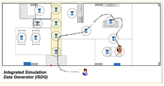
Figure 16.
Example of ISDG-generated data showing subject movement and PIR sensor detections.
5.2. Spatiotempral Data Cleaning Filter
This section outlines the implementation of the proposed method. A flowchart illustrating how the subject’s movement is determined using the PIR sensor network topology and walking speed is presented in Figure 17.
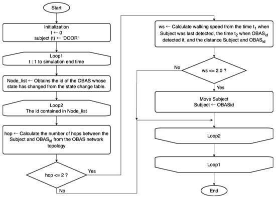
Figure 17.
Algorithm for filtering erroneous data using PIRS network topology and walking speed.
Initially, at , the subject’s location is set at the room entrance (‘DOOR’). As time progresses, the IDs of the PIR sensor units that change from ‘OFF’ to ‘ON’ are stored in the from the PIR sensor state change table. The number of hops between the subject’s current location and each PIRS ID in the is then calculated. If the number of hops is two or less, the walking speed is calculated. Movements with walking speed under 2 m per second are considered correct. However, if the number of hops exceeds three or the walking speed is over 2 m per second, the movement is classified as a false positive.
Figure 18 presents a flowchart for the late-binding method, which filters erroneous data from PIRS units, omitting the number of hops and walking speed calculations shown in Figure 18. At time , when the state changes, the PIR sensor id is added to the . The response varies based on the number of IDs:
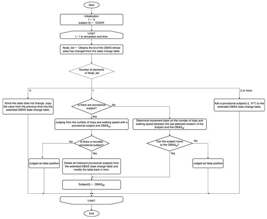
Figure 18.
Flowchart of late-binding data correction process for PIRS units based on the number of detected IDs.
- Zero IDs: No change from the previous state; the state at time is copied to the extended PIRS state change table.
- One ID: Indicates potential subject detection, initiating movement determination. If no provisional subject exists, it is evaluated whether movement from the last detected location to is feasible. If a provisional subject is present and can move to , other provisional subjects are removed, and updates are made retrospectively to the state change table. If movement is not feasible, is flagged as a false positive.
- Two or more IDs: Uncertain movement decision: ‘(, ‘A?’)’ is added as a provisional subject to the extended PIRS state change table.
5.3. Software Development for Converting PIR Sensor Log Data into Trajectory Data
As described in Section 5.2, the LBIS system produces the PIR sensor (PIRS) state change table and subject trajectory data, filtering out erroneous detections from the PIRS time series data. As shown in Figure 19, we developed the software SensorPathFinder using Python to visualize the subject’s movement trajectories.
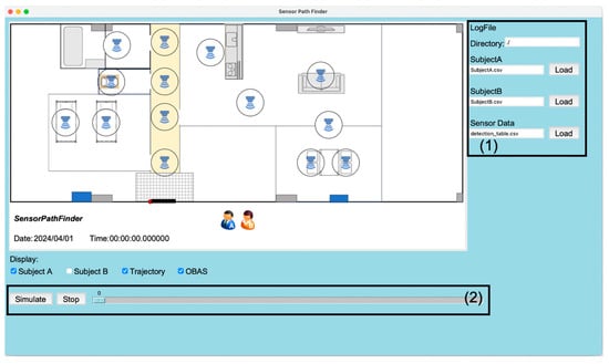
Figure 19.
SensorPathFinder software interface for visualizing subject movement and PIRS data.
5.4. Simulation Scenarios of Error Data Generation from PIRS Units and Their Corrections
The goal of this study is to utilize LBIS to eliminate false positives and omissions in data caused by PIRS units and blocking time, ensuring accurate trajectory identification. To demonstrate this, three scenarios involving PIRS false positives and detection omissions were constructed. Visualizations of each scenario are displayed in the Figure 20. In these scenarios, the performance of a naive method is composed with the proposed LBIS method:
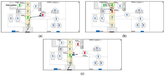
Figure 20.
Simulation scenarios. (a) False positives. (b) Missed detection during blocking time. (c) Simultaneous detection by two PIRS units.
- Case 1: False positive detection by a PIRS unit far from the subject.
- Case 2: Subject reversal during PIRS blocking time.
- Case 3: Simultaneous detection by two PIRS units.
5.5. Evaluation of the Conversion of PIR Sensor Log Data into Trajectory Data
This section presents the simulation results for the three scenarios in Section 5.4.
5.5.1. Case 1: False Positive Detection by a PIRS Unit at a Distance from the Subject
Figure 21 illustrates the results of data cleaning for tracking methods: (a) The naive method—blue plots represent paths generated by ISDG, while green plots show the naive tracking results, including a false positive at the unit, which deviates from the actual trajectory; (b) PIRS network topology and walking speed—red plots depict the path after applying data cleaning with these methods. In Figure 21b, the trajectory closely aligns with the actual path, demonstrating the effectiveness of this approach in correcting false positives.
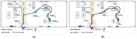
Figure 21.
Tracking results. (a) Naive method with false positives. (b) Data cleaning with PIRS network topology.
5.5.2. Case 2: Subject Reversal During PIRS Blocking Time
Simulation results for a scenario where the subject reversed direction during the PIR sensor blocking time is shown in Figure 22. After passing , the subject turns around at , pass again during the blocking time, and then moves to . In the naive method, depicted in Figure 22a, when the subject is shown moving directly between and , a path does not present in the topology due to the missed detection at . However, with data cleaning using PIRS network topology and walking speed, shown in Figure 22b, the path is correctly adjusted to include a movement through , as direct movement between and is not feasible.
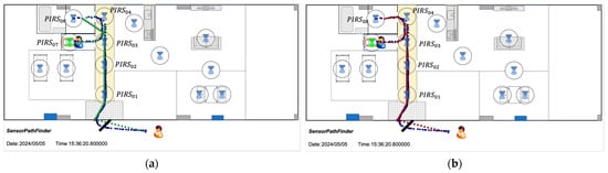
Figure 22.
Simulation results for the case where the subject passed during the blocking time of an PIRS unit. (a) When tracking the raw time-series data from the sensors, if the subject passes through during its blocking time, the system may interpret the movement as a transition from to . (b) By leveraging topology information and constraints based on walking speed, the false negative at was corrected, allowing the system to accurately determine the correct path.
5.5.3. Case 3: Simultaneous Detection by Two PIRS Units
Figure 23 displays tracking results for a scenario where two PIRS units simultaneously detect movement, analyzed through three methods:
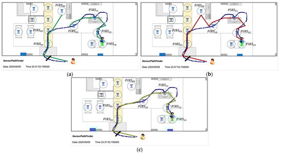
Figure 23.
Simulation results for simultaneous detection by two PIRS units. (a) Naive method tracking. The false positives have not been fixed. (b) and were detected at the same time and, due to the order of processing in the program, , which has the lower index number, was judged to be correct, and was judged to be a false detection. It was judged that the movement was from to based on the topology information, and was inserted as the route in the middle. (c) Because and are being detected at the same time, a candidate for movement form to and is created. The LBA then determines that is a false positive based on the next detection, .
- Naive method (Figure 23a): The trajectory starts at , which has the smallest ID, and then moves to . No path exists between and due to simultaneous detections, suggesting the subject moves to immediately upon arriving at .
- Network topology and walking speed (Figure 23b): This analysis chooses over , both detected simultaneously, due to its smaller ID. is deemed a false positive because there is no time lapse between the subject moving from . The movement from to then follows a two-hop path via , reflecting the absence of a direct link in the network topology.
- Late-binding approach (Figure 23c): This method refines the tracking by correcting discrepancies observed in simpler methods, aligning the trajectory closely with the actual movement path.
6. Evaluation Using Real-World Experiments
Evaluating any proposed system or framework is essential to confirm its effectiveness and applicability in real-world settings. Although initial validation of our late-binding system (LBIS) for correcting inaccurate detections in sensor data occurred through simulations, it is crucial to test its robustness in practical settings with actual participants. This section discusses transitioning from theoretical analysis and simulations to implementing the LBIS framework in a real-world scenario. We will use three participants in a controlled environment that mimics typical the living conditions of elderly individuals.
The primary goal of this real-world evaluation is to determine the effectiveness and reliability of the LBIS system under the uncontrolled variables and dynamic conditions typical of practical applications. The focus is on assessing how accurately the system detects movements, eliminates false positives, and tracks the trajectories of elderly individuals using commercially available PIR sensors.
By comparing real-world test results with simulation data, we aim to identify the strengths and limitations of the LBIS framework. This comparative analysis helps highlight where the system excels and where it needs further refinement. Through this approach, the evaluation offers a comprehensive understanding of the LBIS framework’s capabilities and its potential for deployment in residential settings for elderly monitoring. The following subsections will detail the experimental setup, present results from real-world tests, and provide a comparative analysis between simulated and actual data, discussing any deviations and their potential causes.
6.1. Real-World Experiment Setup and Participants for Spatiotemporal Cleaning of PIR Sensor Data
The real-world experiment was carefully designed to mimic the daily conditions experienced by elderly individuals, testing the practical applicability of the LBIS framework. The study included three participants aged between 65 and 72, representing typical mobility patterns seen in older adults. Participants engaged in everyday activities such as walking, sitting, and moving between rooms within a controlled environment modeled after a residential setting.
Since the map used in the simulation was narrow and space was still available, the layout was changed to use the entire room and sensors were added. The layout of the real-world experiment is shown in Figure 24.
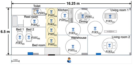
Figure 24.
Layout of the room used in the real-world experiment.
The experimental setup replicated a typical household environment, including a living room, kitchen, hallway, and bedroom. PIR sensors were strategically positioned at key locations, such as doorways and corridors, and near frequently used furniture to ensure comprehensive monitoring of participants’ movements. The sensor layout was optimized to consider potential obstacles like furniture that could interfere with sensor signals, thereby enhancing the system’s accuracy.
Special care was taken to optimize the PIR sensors for peak performance. Calibration was conducted to minimize false positives due to environmental factors such as changes in room temperature or lighting conditions. The experiment was designed to control variables like the time of day, collecting data under both daylight and artificial lighting. Each participant’s movement was tracked across multiple sessions, each lasting about an hour, to ensure a robust dataset for analysis.
To maintain data integrity, the system’s edge computer synchronized all sensor inputs using a network time protocol (NTP) server, minimizing time lags and enhancing movement tracking precision. This synchronization was crucial for maintaining the temporal consistency essential for the LBIS framework to accurately determine movement trajectories and filter out false positives. This comprehensive setup facilitated a thorough evaluation of the LBIS system under realistic conditions, providing valuable insights into its real-world performance.
6.2. Results from Real-World Testing
The real-world implementation of the LBIS framework yielded valuable data that validated its performance. Compared to the simulation, there were multiple false positives and false negatives in the actual data, but the LBIS system was able to eliminate these errors and accurately track the movement of the elderly in real-life situations.
During the experiment, compared to the naive method of tracking based on the time series data of the PIR sensor, the LBIS framework was able to reduce the average error to around 1.0 m from the correct route, proving the reliability of mapping the spatial patterns of the elderly. The system also achieved over 90% accuracy in tracking participants’ movement trajectories, proving its reliability in mapping the spatial patterns of elderly individuals.
In real-world test, because the sensor’s detection range was limited, if the subject moved to the boundary of the detection range, there was a possibility of a false negative, where the sensor did not detect the subject. In fact, in in Figure 25, there were cases where a false negative was detected when the subject passed close to the wall when entering the room on the right; however, it was possible to correct the false negatives and extract the correct path using the LBIS framework.
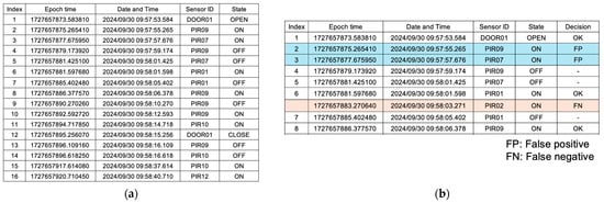
Figure 25.
Raw data logs and spatiotemporal cleaning results from real-world experiments: two cases of false positives and false negatives. (a) Raw data logs form sensors. (b) Walking speed constraint: set to less than 2.0 m/s; Number of hops limit: set to two hops or less. In No. 2, the walking speed is 3.5 m/s, and in No. 3, it is 1.7 m/s but four hops; therefore, these are determined as false positives. Although and are not adjacent, since the walking speed is reasonable (less than 2.0 m/s), in the intermediate path is determined to be a false negative.
Real-world data highlighted the system’s efficiency in handling simultaneous detections from multiple sensors, common in densely monitored environments. The late-binding adjustment (LBA) was key in retroactively correcting data inaccuracies, ensuring that the final trajectory closely matched actual movements. These results confirm the LBIS framework’s practical applicability and its potential to improve elder care technologies with more accurate and reliable movement monitoring in residential settings.
6.3. Comparative Analysis: Simulation vs. Real-World Results
The comparative analysis between simulation results and real-world experiment outcomes offered valuable insights into the LBIS framework’s performance consistency. Both approaches showed high accuracy in tracking elderly movements, though some differences were noted, likely due to the variability inherent in real-world conditions.
In simulations, the LBIS system achieved near-perfect accuracy with almost zero false positives and negatives, as simulations lack uncontrolled variables. However, in real-world tests, while the system’s performance remained strong, slight deviations in data accuracy occurred due to factors like sensor placement, environmental interferences, and participants’ physical conditions. For example, when participants moved unusually slowly or paused unexpectedly, minor inconsistencies in sensor data were observed, which were less common in the controlled simulation environment.
The LBA’s effectiveness was also compared across the two scenarios. In simulations, the algorithm quickly adapted to data changes and corrected inaccuracies seamlessly due to idealized inputs; however, in the real-world implementation, it required additional processing time to manage more complex movement patterns and overlapping sensor signals, revealing opportunities for algorithmic refinements to improve system responsiveness.
Despite these differences, the comparative analysis confirmed that the LBIS framework’s core functions—error correction and trajectory mapping—remained highly reliable in both simulated and real-world environments. The slight variations in data handling highlight the need for ongoing refinement and testing of the LBIS algorithm in diverse settings to optimize its performance. This analysis demonstrates the LBIS framework’s potential as a robust tool for real-world elderly monitoring systems, supporting its integration into broader healthcare and smart home solutions.
Figure 26 visualizes the tracking results based on sensor data obtained from actual measurements, comparing four methods: the Naive method that tracks raw time-series data (Figure 26a), a method combining the Naive approach with network topology (Figure 26b), a method that limits tracking to a maximum of two hops and a walking speed of 2.0 m/s (Figure 26c), and the proposed method (NDT + LBA) (Figure 26d). In the figure, the green plots represent the actual positions of the subject derived from video footage during the measurement, while the red plots indicate the positions generated from the sensor data. The green and red plots corresponding to the same time are connected by black lines, representing the errors between the two points. The white plots interpolate the positions between green plots at 0.1-s intervals. In the proposed method (Figure 26d), it is visually confirmed that tracking is performed with minimal error.
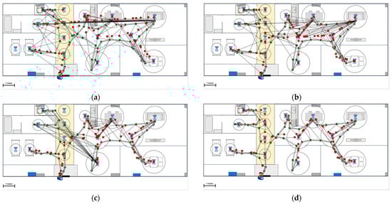
Figure 26.
Visualization of the spatiotemporal cleaning results for real PIR sensor log data and the actual trajectory data generated from video camera recordings. (a) Results of tracking by naive method without network topology. (b) Results of tracking by naive method with network topology. (c) Results filtered by hop count and walking speed. (d) Results of combining late binding.
Additionally, Table 2 presents the average error, maximum error, minimum error, and standard deviation based on data from three subjects, showing that proposed Late Binding method improves all error metrics. Furthermore, Table 3 shows the number of false positive and false negative data points in the raw data and the number of corrected data point using the proposed method, demonstrating the effectiveness of the filtering process.
Table 2.
Error between the actual trajectory and the simulated trajectory generated from the PIR sensor data after spatiotemporal cleaning.
Table 3.
The number of false positives and false negatives in the raw data, and the number of corrections made by late binding.
7. Discussion
The real-world experiments closely matched simulation predictions, confirming the LBIS system’s effectiveness in practical settings. The experiments showed that the system successfully filtered out false positives detected by the PIR sensors and achieved over 90% accuracy in tracking elderly participants’ movements, validating its viability in real residential environments. This paper introduces a method for tracking based on inaccurate time series data from PIR sensor units, addressing issues like false and missed detections often caused by sensor limitations like blocking times. One approach leverages the sensor network topology, incorporating sensor layout and walking speed between units. The late-binding method addresses uncertain states, such as simultaneous detections, making corrections upon subsequent confirmations. Combining these methods has proven effective, demonstrating accurate tracking even in scenarios where PIR sensors alone are insufficient.
Although the tracking in this study is less detailed than in related work due to its reliance on network topology, it still effectively estimates activity based on indoor movement and detection frequency. With time-synchronized sensor nodes (PIRS units), walking speed can be measured from travel time between nodes, making the system fully functional for monitoring elderly individuals in their homes.
In this study, movement between sensors is represented as a straight line, leading to coarser accuracy compared to other tracking technologies. However, the system effectively monitors elderly activity by quantitatively measuring indoor movement and the number of sensor detections, as well as calculating walking speed between sensors. Continuous monitoring enables early detection of changes in health status, simply by observing daily activities at home. Since PIR sensors do not record video, privacy concerns are minimized, and their mass production allows for cost-effective implementation.
We proposed a system for tracking indoor movement in the homes of elderly individuals living alone or with a partner. Since PIR sensors only detect human presence or absence, applying this system in crowded settings like nursing homes is challenging. However, it is well-suited for monitoring movements in private rooms. In the future, we plan to develop scenarios involving two people indoors to evaluate the tracking system. We will verify the system on actual devices based on simulation results.
The simulation environment used in this study is designed to model behaviors in a real household setting; however, it cannot fully replicate the complexities of real-world environments, such as temperature fluctuations, furniture arrangements, walls, and human movement. Therefore, to further evaluate the effectiveness of the proposed method in real-world scenarios, experiments in more diverse real environments are necessary.
The dataset used in this study was obtained from three participants, which limits its scale and diversity. Thus, we believe validation using a larger dataset that includes various living environments is required.
The proposed non-deterministic tracking (NDT) and late-binding adjustment (LBA) algorithms can impose a high computational load in cases with an increased number of sensors of frequent false detections. This may affect their real-time applicability, particularly on resource-constrained edge devices. In the future, we aim to improve real-time performance through the quantitative measurement of computational load and optimization of the algorithms.
In Wu et al.‘s study [9], PIR sensors are densely placed, and data from multiple sensors are combined to correct false detections. However, this method tends to be cost-intensive due to the large number of sensors required. In contrast, our study achieves high-accuracy data cleaning while minimizing the number of sensors by combining NDT with LBA. Ngamakeur et al. adopted a machine learning-based approach using accelerometers and Bluetooth Low Energy (BLE) scanners, achieving high-accuracy activity recognition [11]. However, these methods consume significant computational resources, making real-time processing on low-cost edge devices challenging. Our method improves computational efficiency with a simple algorithm, allowing it to function in resource-limited environments. Additionally, as the system is device-free for elderly users, it enables measurement through normal daily activities, reducing their burden. This study provides a low-cost, non-intrusive solution suitable for real-time processing. By effectively correcting false detections and missed detections, our method offers higher flexibility and applicability compared to conventional approaches. We believe this enhances the reliability of motion monitoring in elderly living environments and provides valuable information for caregivers and healthcare professionals.
8. Conclusions
This paper addresses the challenges associated with using passive infrared (PIR) sensors for elderly monitoring in indoor environments, specifically focusing on handling inaccuracies such as false positives and false negatives. To effectively mitigate these issues, we proposed an integrated approach that combines non-deterministic tracking (NDT) and late-binding adjustment (LBA). NDT provides the system with the flexibility to hypothesize multiple movement paths in real-time, allowing it to handle the uncertainty present in dynamic environments. LBA, on the other hand, retroactively corrects these initial hypotheses based on new sensor data, ensuring that the final movement paths are as accurate as possible. Together, these algorithms form a dynamic and adaptive framework that achieves a balance between real-time flexibility and long-term accuracy, enhancing the system’s ability to track indoor movements in complex environments with sensor-based uncertainties.
To validate this approach, we introduced a novel spatiotemporal cleaning framework that utilizes the sensor network topology alongside the LBA, improving data reliability for elderly care monitoring. Simulations demonstrated the effectiveness of this method in filtering erroneous data and accurately tracking indoor movement. Moreover, real-world testing with three participants confirmed the practical applicability of the late-binding system (LBS) for correcting inaccurate detections in the sensor data framework, achieving high accuracy in detecting and tracking movement and highlighting its potential for deployment in elderly care settings. This integrated approach significantly reduces false positives and retroactively corrects incomplete data, addressing the critical challenges in sensor-based monitoring applications for elderly homes.
Future research should explore further the integration of different types of sensors, such as combining PIR sensors with acoustic or other sensor technologies, to create a more robust and multifaceted system. Additionally, developing real-time adaptive algorithms that adjust sensor sensitivity based on contextual factors like time of day or activity level could further enhance system performance. Expanding real-world testing across diverse elderly populations will also help refine the technology to ensure its effectiveness in varied living environments, ultimately contributing to more reliable and precise monitoring solutions for elderly care.
The current framework is based on PIR sensors, but integrating other low-cost ambient sensors, such as ultrasonic sensors, is expected to improve detection accuracy by reducing false detections and missed detections. Additionally, this integration could expand the applicability to scenarios involving multiple individuals. Such enhancements are anticipated to further improve tracking accuracy and enable applications in more complex environments. Integrating the proposed method into an IoT-based comprehensive elder care system could facilitate real-time health monitoring and anomaly detection. This system is expected to be applicable not only in home environments but also in diverse settings such as nursing homes and hospitals. While the current framework primarily targets residential environments, future work will explore its application in clinical settings, including hospitals and rehabilitation facilities. This would enable the monitoring of patient mobility and activities, contributing to the establishment of an efficient and rapid response system for healthcare staff.
Author Contributions
Conceptualization, T.U. and M.A.; methodology, T.U. and M.A.; software, T.U.; validation, T.U. and M.A.; formal analysis, T.U. and M.A.; data curation, T.U.; writing—original draft preparation, T.U.; writing—review and editing, M.A.; visualization, T.U.; supervision, M.A.; project administration, M.A. All authors have read and agreed to the published version of the manuscript.
Funding
This research was funded by JSPS KAKENHI, grant number JP24K15631.
Institutional Review Board Statement
The study was conducted in accordance with the Declaration of Helsinki, and the protocol was approved by the Ethics Committee of Akita University based on Article 6, Paragraph 2 of the Ethical Guidelines for Research Involving Human Subjects in the Tegata Campus Area (Approval Number: 6-42).
Informed Consent Statement
Informed consent for participation was obtained from all subjects involved in the study.
Data Availability Statement
The data presented in this study are available on request from the corresponding author due to privacy.
Conflicts of Interest
The authors declare no conflicts of interest.
References
- World Health Organization. Aging and health. Available online: https://www.who.int/news-room/fact-sheets/detail/ageing-and-health (accessed on 29 February 2024).
- Enssle, F.; Kabisch, N. Urban green spaces for the social interaction, health and well-being of older people—An integrated view of urban ecosystem services and socio-environmental justice. Environ. Sci. Policy 2020, 109, 36–44. [Google Scholar] [CrossRef]
- Uddin, M.Z.; Khaksar, W.; Torresen, J. Ambient Sensors for Elderly Care and Independent Living: A Survey. Sensors 2018, 18, 2027. [Google Scholar] [CrossRef] [PubMed]
- Tomii, S.; Ohtsuki, T. Falling detection using multiple doppler sensors. In Proceedings of the 2012 IEEE 14th International Conference on e-Health Networking, Applications and Services (Healthcom), Beijing, China, 10–13 October 2012; pp. 196–201. [Google Scholar] [CrossRef]
- Rajavel, R.; Ravichandran, S.K.; Harimoorthy, K.; Nagappan, P.; Gobichettipalayam, K.R. IoT-based smart healthcare video surveillance system using edge computing. J. Ambient Intell. Humaniz. Comput. 2022, 13, 3195–3207. [Google Scholar] [CrossRef]
- Jo, T.H.; Ma, J.H.; Cha, S.H. Elderly Perception on the Internet of Things-Based Integrated Smart-Home System. Sensors 2021, 21, 1284. [Google Scholar] [CrossRef]
- Shah, S.A.; Ahmad, J.; Masood, F.; Shah, S.Y.; Pervaiz, H.; Taylor, W.; Imran, M.A.; Abbasi, Q.H. Privacy-Preserving Wandering Behavior Sensing in Dementia Patients Using Modified Logistic and Dynamic Newton Leipnik Maps. IEEE Sens. J. 2021, 21, 3669–3679. [Google Scholar] [CrossRef]
- Sugianto, N.; Tjondronegoro, D.; Stockdale, R.; Yuwono, E.I. Privacy-preserving AI-enabled video surveillance for social distancing: Responsible design and deployment for pbulci spaces. Inf. Technol. People 2024, 37, 998–1022. [Google Scholar] [CrossRef]
- Wu, C.M.; Chen, X.Y.; Wen, C.Y.; Sethares, W.A. Cooperative Network PIR Detection System for Indoor Human Localization. Sensors 2021, 21, 6180. [Google Scholar] [CrossRef] [PubMed]
- Tabbakha, N.E.; Ooi, C.-P.; Tan, W.-H.; Tan, Y.F. A wearable device for machine learning based elderly’s activity tracking and indoor location system. Bull. Electr. Eng. Inform. 2021, 10, 927–939. [Google Scholar] [CrossRef]
- Ngamakeur, K.; Yongchareon, S.; Yu, J.; Islam, S. Passive infrared sensor dataset and deep learning models for device-free indoor localization and tracking. Pervasive Mob. Comput. 2023, 88, 101721. [Google Scholar] [CrossRef]
- Tao, S.; Kudo, M.; Pei, B.N.; Nonaka, H.; Toyama, J. Multiperson Location and Their Soft Tracking in a Binary Infrared Sensor Network. IEEE Trans. Hum. Mach. Syst. 2015, 45, 550–560. [Google Scholar] [CrossRef]
- Veronese, F.; Comai, S.; Mangano, S.; Matteucci, M.; Salice, F. PIR Probability Model for a Cost/Reliability Tradeoff Unobtrusive Indoor Monitoring System, Lecture Notes of the Institute for Computer Sciences. In Proceedings of the International Conference on Smart Objects and Technologies for Social Good, Pisa, Italy, 29–30 November 2017; p. 61. [Google Scholar] [CrossRef]
- Shokrollahi, A.; Persson, J.A.; Malekian, R.; Sarkheyli-Hägele, A.; Karlsson, F. Passive Infrared Sensor-Based Occupancy Monitoring in Smart Buildings: A Review of Methodologies and Machine Learning Approaches. Sensors 2024, 24, 1533. [Google Scholar] [CrossRef] [PubMed]
- Khan, D.S.; Kolarik, J.; Hviid, C.A.; Weitzmann, P. Method for long-term mapping of occupancy patterns in open-plan and single office spaces by using passive-infrared (PIR) sensors mounted below desks. Energy Build. 2021, 230, 110534. [Google Scholar] [CrossRef]
- Sultanabanu, K.; Liyakat, S.; Kazi, K.; Kosgiker, G.; Gund, V. PIR Sensor-Based Arduino Home Security System. Int. J. Eng. Res. Technol. 2019, 8. [Google Scholar]
- Masciadri, A.; Lin, C.; Comai, S.; Salice, F. A Multi-Resident Number Estimation Method for Smart Homes. Sensors 2022, 22, 4823. [Google Scholar] [CrossRef] [PubMed]
- Narayana, S.; Prasad, R.V.; Rao, V.S.; Prabhakar, T.V.; Kowshik, S.S.; Iyer, M.S. PIR Sensors: Characterization and Novel Localization Technique. In Proceedings of the 14th International Conference on Information Processing in Sensor Networks, Seattle, WA, USA, 13–16 April 2015; pp. 142–153. [Google Scholar] [CrossRef]
- Sakai, H.; Okuma, H.; Wu, M.; Nakata, M. Rough Non-Deterministic Information. In The Handbook on Reasoning-Based Intelligent Systems; World Scientific Publishing Co Pte Ltd.: Singapore, Singapore, 2013; pp. 81–118. [Google Scholar] [CrossRef]
- Sakai, H.; Nakata, M. On Possible Rules and Apriori Algorithm in Non-deterministic Information Systems. In Rough Sets and Current Trends in Computing; RSCTC 2006—Lecture Notes in Computer Science; Greco, S., Ed.; Springer: Berlin/Heidelberg, Germany, 2006; Volume 4259. [Google Scholar] [CrossRef]
- Taylor, J.T.; Taylor, W.T. More About Late Binding. In Patterns in the Machine; Apress: Berkeley, CA, USA, 2021. [Google Scholar] [CrossRef]
- Pontelli, E.; Ranjan, D.; Gupta, G. The Complexity of Late-Binding in Dynamic Object-Oriented Languages. In Principles of Declarative Programming, ALP PLILP 1998—Lecture Notes in Computer Science; Palamidessi, C., Glaser, H., Meinke, K., Eds.; Springer: Berlin/Heidelberg, Germany, 1998; Volume 1490. [Google Scholar] [CrossRef]
- Utsumi, T.; Arikawa, M.; Hashimoto, M. MUS3E: A Mobility Ubiquitous Sensor Edge Environment for the Elderly. Electronics 2023, 12, 3003. [Google Scholar] [CrossRef]
- Akizuki Denshi Tsusho. SB612B Datasheet. Available online: https://akizukidenshi.com/goodsaffix/SB612B_20221128.pdf (accessed on 5 March 2024).
- ROBU.IN. Pyroelectric Infrared Radial Sensor. Available online: https://robu.in/wp-content/uploads/2020/09/Pir-BM612.pdf (accessed on 5 March 2024).
- Yoshimura, N.; Muraki, S.; Oka, H.; Tanaka, S.; Ogata, T.; Kawaguchi, H.; Akune, T.; Nakamura, K. Association between new indices in the locomotive syndrome risk test and decline in mobility: Third survey of the ROAD study. J. Orthop. Sci. 2015, 20, 896–905. [Google Scholar] [CrossRef]
- Hirai, T.; Chidori, K.; Watanabe, N.; Hoshino, M.; Kawai, H.; Ueno, N.; Inoue, D.; Harada, T.; Maki, K.; Shimoto, T. Evaluation of the Grading Ability of Walking Speed by the Elderly. J. Phys. Ther. Sci. 2008, 23, 711–715. [Google Scholar] [CrossRef][Green Version]
Disclaimer/Publisher’s Note: The statements, opinions and data contained in all publications are solely those of the individual author(s) and contributor(s) and not of MDPI and/or the editor(s). MDPI and/or the editor(s) disclaim responsibility for any injury to people or property resulting from any ideas, methods, instructions or products referred to in the content. |
© 2024 by the authors. Licensee MDPI, Basel, Switzerland. This article is an open access article distributed under the terms and conditions of the Creative Commons Attribution (CC BY) license (https://creativecommons.org/licenses/by/4.0/).