Abstract
To address the uncertainty in the statistical distribution model of positioning error for the accuracy test of long-endurance inertial navigation systems, a probability distribution model adheres to the statistical rule of the radial positioning error of inertial navigation systems. The probability distribution density function (PDF), cumulative density function (CDF), and characteristic numbers (mean, standard deviation, root-mean-square) of the radial positioning error are derived based on the static-base positioning error of the long-range inertial navigation systems. Methods are provided for estimating the parameters of the probability distribution of the radial positioning errors. The theoretical derivation results demonstrate that the radial positioning error follows the Hoyt distribution. The distribution parameters and the number of features grow linearly with time, while the mean and standard deviation converge to 60% and 80% of the root-mean-square, respectively. Through a large-sample Monte Carlo simulation, the experimental results were consistent with the theoretical derivation results. These results indicate that the theoretical derivation results can be used to optimize the design of the long-endurance rotary modulation inertial navigation system’s accuracy test.
1. Introduction
With the improvement in the accuracy of gyroscopes and accelerometers and the development of the technology to compensate for the system’s errors, the time needed to maintain the accuracy of inertial navigation systems becomes longer and longer, which causes the cost of the long-endurance accuracy test of the inertial navigation systems to rise sharply and the test time to increase dramatically [1]. On the one hand, the development of inertial technology has improved the ability of inertial navigation systems to maintain accurate working time [2]; on the other hand, the demand of inertial navigation systems users has led to the extension of autonomous working time [3,4].
The positioning error of a long-endurance dual-axis rotary modulation inertial navigation system involves randomness of launch and regularity of inherent period oscillation [5]. Randomness means that independent test samples must be taken repeatedly with the power off, while regularity helps to analyze the trend of the positioning error over time. In the previous positioning accuracy test of the short-endurance inertial guidance system, it was usually assumed that the randomness of the positioning error of the inertial navigation systems would obey the normal distribution according to the Law of Large Numbers. The inertial navigation system’s positioning accuracy test program is formulated on this basis, involving selecting the number of test samples and evaluating accuracy indices. In practice, the limited number of test samples for long-endurance dual-axis rotary modulation inertial navigation systems makes it challenging to satisfy the sample size requirement of the normality assumption, and the radial positioning error is non-negative, which is modeled as inconsistent with the probability distribution model, where the normal distribution can cover both positive and negative ranges. Continuing to use the normal distribution to estimate accuracy metrics will result in positioning accuracy assessment results that do not match actual performance levels. In addition, the inherent oscillation law of the positioning error of the inertial navigation systems was ignored in the design of the test program, resulting in inadequate analysis of the test data. Therefore, to optimize the design of the long-endurance inertial navigation accuracy test, it is necessary to study the probability distribution model that satisfies the radial positioning error law of the long-endurance dual-axis rotary modulation inertial navigation systems.
The error propagation of inertial navigation systems is essentially a complex time-varying system strongly influenced by the motion state of the attitude vehicle [4]. Generally, the dynamic baseline test data evaluation is guided by the stationary base error law of the inertial navigation system [6]. Based on the actual application of long-endurance inertial navigation, gyroscopic drift is the main factor influencing the error of long-endurance inertial navigation systems, while initial pointing and accelerometer errors have negligible influence on the system error [7]. Among them, gyroscopic zero-bias repeatability, zero-bias stability, and random wander coefficient are essential indicators of gyroscopic accuracy performance, determining the upper limit of inertial navigation systems’ accuracy.
Rotational modulation technology mitigates the impact of most slow-changing gyroscope errors on the positioning error of inertial navigation systems. However, random walks still cannot be modulated, and temperature variations, carrier maneuvering, and other factors cause non-random errors. For use scenarios with small ambient temperature changes and infrequent carrier maneuvering, the non-random errors caused by gyroscopes are relatively stable. To simplify the analysis, the residual errors of the non-random errors of gyroscopes that are not fully modulated are equivalent to the angular velocity drift of gyroscopes and are assumed to be random constants [8]. There are clear conclusions on the statistical analysis of random walks on the positioning error of inertial navigation systems, but the statistical results of non-random errors of gyroscopes on positioning errors have not been reported. Therefore, this paper focuses on studying the probability distribution model of positioning errors caused by equivalent constant drift of gyroscopes under the condition of a stationary base for long-endurance dual-axis rotational modulation inertial navigation systems and establishes a probability distribution model of radial positioning errors for long-endurance inertial navigation systems based on this.
The rest of the paper is structured as follows. Section 2 analyzes the randomness and regularity of the positioning error in the actual use of a long-endurance dual-axis rotary modulation inertial navigation system; Section 3 derives the probability distribution of the latitude, longitude, and radial positioning error under the static base condition of long-endurance inertial navigation; Section 4 derives the proof that the long-range radial positioning error conforms to the Hoyt distribution model, and gives the eigenvalue function of the Hoyt distribution as well as the estimation method of the model parameters; Section 5 discusses the dual precision indicators and calculation methods of long-endurance inertial navigation systems; and Section 6 validates the long-endurance inertial navigation system’s radial positioning error through the Large Sample Monte Carlo and verifies that the radial positioning error under the static base condition of long-endurance inertial navigation conforms to the Hoyt distribution model. Section 7 summarizes the entire content.
2. Analysis of Long-Endurance Inertial Navigation System Positioning Error
Long-endurance inertial navigation is mainly applied to concealed carriers for underwater navigation [9]. The primary navigation state involves obtaining external velocity through the assistance of a log for damping [10,11]. This article mainly discusses long-endurance inertial navigation systems working in a damping state.
For long-term navigation of low-speed carriers, the propagation characteristics of systematic errors can be analyzed using the static base positioning error equation. The static base positioning error equation for dual-axis rotation-modulated inertial navigation is reconstructed as shown in Equations (1) and (2).
Let , we have:
where and represent latitude and longitude; and represent latitude errors and longitude errors; are the equivalent gyroscope angular velocity drift values caused by incomplete modulation in the east, north, and sky directions; is the Earth’s rotation rate; is the Schuler angular frequency; and is the Foucault angular frequency.
According to Equations (1) and (2), it can be seen that the positioning error of the inertial navigation systems mainly manifests as the Schuler oscillation error, Earth oscillation error, and cumulative divergence error over time. The Schuler oscillation error can be suppressed into a small amount of error through velocity-damping technology. Equations (1) and (2) can be simplified as follows:
The analysis of positioning errors in the OPEQ coordinate system (as shown in Figure 1 and Figure 2) is more concise [12]. The OPEQ coordinate system is often used in INS retuning/correction methods. Its origin is at the center of mass of the carrier; the E-axis is tangent to the latitude circle where the carrier is located and points east; the P-axis is oriented along the polar axis; and the Q-axis, which forms a right-handed rule with the E-axis and the P-axis, points to the plane of the latitude circle. The projection of equivalent gyroscope error in the OPEQ system is , and the mapping relationship is shown in Equation (5). Equations (3) and (4) can be simplified using Equation (5) to obtain the error equation of inertial positioning error in the OPEQ coordinate system, as shown in Equations (6) and (7).
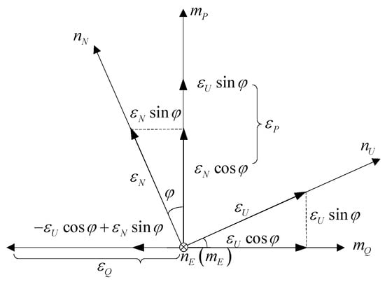
Figure 1.
Conversion diagram between the OPEQ coordinate system and navigation (N) coordinate system.
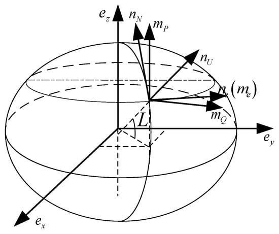
Figure 2.
Diagram of the relationship between the OPEQ coordinate system and the N coordinate system.
It is easy to conclude from Equation (8) that the phase of latitude oscillation error lags 90 ° behind that of longitude oscillation error.
3. Probability Distribution of Long-Endurance Inertial Navigation Positioning Error
In the previous section, we analyzed the positioning error of long-endurance inertial navigation under static base conditions and provided the projection results in the OPEQ system. From Equations (6) and (7), it can be seen that the statistical characteristics of equivalent gyro drift determine the statistical characteristics of long-endurance inertial navigation positioning errors. The equivalent gyro drift is affected by the gyro error characteristics, rotation modulation scheme, initial alignment process, etc. Generally, it can be assumed that follow a normal distribution of zero mean and standard deviation and are independent of each other, i.e., , , . From the linear additivity of a normal distribution, it can be concluded that , i.e., \ still follows a normal distribution with zero means, and \\ are independent of each other.
3.1. PDF of Latitude Errors and Longitude Errors
Firstly, we analyze the probability distribution of latitude error and perform the following binary transformation:
The corresponding Jacobian determinant is shown in Equation (11):
According to the independence of between , there are
Then:
The marginal probability density function of two-dimensional random variables and is:
From Equations (13)–(15), can be easily obtained. If the joint probability density function of two-dimensional random variables and is equal to the product of the marginal probability density function, it can be obtained that the random variables and are independent of each other. The distribution of Equation (14) is called a Rayleigh distribution, where the amplitude of latitude error follows a Rayleigh distribution and the phase follows a uniform distribution.
Furthermore, based on the probability density distribution functions and independence of and , the probability characteristics of the random signal are derived using the supplementary variable method, as shown in Equation (16).
where is the random phase signal and R is the random amplitude following a Rayleigh distribution with parameter . is the random phase following a uniform distribution with , and is the determined angular frequency.
Let:
Jacobian determinant of Equation (17):
According to the calculation formula of the binary joint density function:
From Equation (17), it can be found that:
Then:
By substituting Equation (21) into (19), it can be found that:
where and Equation (22) is the two-dimensional normal probability density function with zero mean. It is easy to conclude that both and follow .
According to the linear additivity of a normal distribution, it can be concluded that both latitude and longitude error random variables follow a normal distribution, and the variance of longitude error random variables increases over time, which is consistent with the divergence trend of longitude errors over time, as shown in Equation (23).
3.2. PDF of Radial Positioning Error
Based on Equation (23), the statistical properties of the radial positioning error random variable given in Equation (24) are discussed. The radial positioning error random variable can also be viewed as the mode of two random variables obeying normal distribution. However, unlike the Rayleigh distribution, the standard deviations of the two normal distribution random variables are different, and the longitude error’s standard deviation diverges over time.
Firstly, the independence between the latitude error random variable and the longitude error random variable is discussed: the independence between and depends on the independence of the random variable between the random variable . The results of (22) have the following implications:
From Equation (25), it can be seen that the correlation between and varies with the interval at any time. Only when does exist, that is, when , are the random variables and independent of each other. When , is a two-dimensional normal distribution density function, as shown in Equation (26), with marginal distributions of and . From the independent random variables between , it can be concluded that the latitude error and longitude error are independent of each other.
When the latitude error random variable and the longitude error random variable are independent of each other, the probability distribution functions of the random variables for and can be derived using the double integral variable variation method.
Let ,, we have:
The joint probability distribution density function of radial positioning errors and corresponding phase is:
The probability density function of is:
where is the first type of modified zero-order Bessel function. The distribution in the form of Equation (28) is called the Hoyt distribution [13].
The PDF of radial positioning error is transformed into a standard Hoyt distribution form [14]:
where , and .
The surface plot of the probability density function over time with = 0.001°/h is shown in Figure 3. From the figure, it can be seen that, at the beginning of time, is concentrated near 0. As time progresses, the probability density surface becomes flat and the dispersion becomes larger, indicating that the positioning accuracy of the inertial navigation systems is deteriorating, consistent with the characteristics of the inertial navigation systems positioning error, which is cumulative over time. Figure 4 further shows the trend over time.
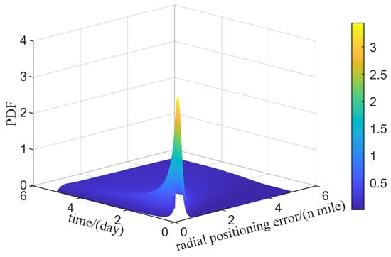
Figure 3.
PDF of radial positioning error over time.
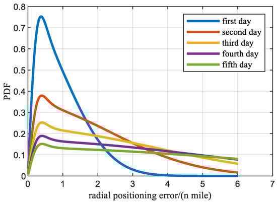
Figure 4.
PDF of radial positioning error in a typical moment.
4. The Distribution Function and Characteristic Number of Radial Positioning Errors
The CDF of a random variable is an integral of the PDF, which is used to calculate the quantile of a random variable. In addition, the mean, standard deviation, and root mean square can be calculated from the distribution. Each of these measures describes the characteristics of the distribution from one side. The mean usually describes the central trend of errors in inertial navigation systems, the standard deviation usually describes the dispersion of errors in inertial navigation systems, and the root mean square combines the characteristics of both. This section introduces the distribution function, characteristic numbers of inertial radial positioning errors, and parameter estimation methods.
4.1. CDF of Radial Positioning Error
The CDF of Hoyt distribution:
The calculation of the Hoyt distribution function, as shown in Equation (30), involves the integration of the Bessel function, and the calculation process is relatively complex. References [15,16] provides a closed-form calculation formula for CDF of Hoyt distribution, as shown in Equation (31). Figure 5 shows the cumulative probability density of the random variable of radial positioning error over time, and Figure 6 further illustrates the cumulative probability density curve at typical moments.
where ; ; is the first-order Marcum-Q function, as shown in Equation (32).
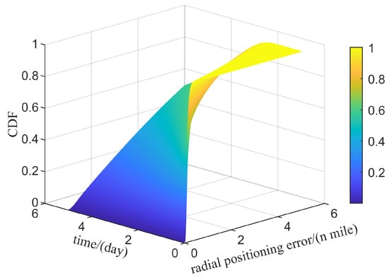
Figure 5.
CDF of radial positioning error over time.
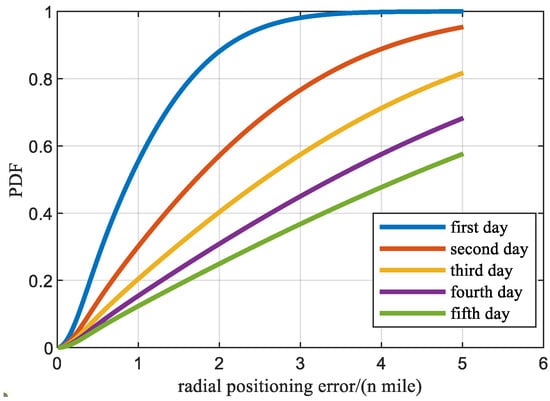
Figure 6.
CDF of radial positioning error in a typical moment.
4.2. Characteristic of Radial Positioning Error
The mean of the radial positioning error is given by [17]:
where is the second type of complete elliptic integral [18].
The standard deviation of radial positioning error:
For the radial positioning error, while paying attention to its root mean square (RMS) trend over time [19], according to the definition of RMS, we have:
From the relationship between gamma distribution and normal distribution, as well as the linear relationship of gamma distribution, it is easy to obtain:
By substituting Equation (37) into Equation (35), we have:
From Equation (38), it can be seen that the RMS of the long-endurance inertial navigation positioning error can be approximated as the linear divergence over time, and the divergence angle depends on the local latitude and equivalent gyro bias . At the same time, it can also be seen that the root mean square of the radial positioning error diverges faster with increasing latitude.
As time t increases, approaches 0, and there are:
Substituting Equation (39) into Equation (33) and Equation (30) we have:
4.3. Estimation of Radial Positioning Error Parameters
has a unique parameter, which is the equivalent gyro bias . Due to the existence of a Bessel function in the Hoyt distribution without a closed solution [20], general parameter estimation methods such as moment estimation and maximum likelihood estimation are challenging to apply. But from Equation (38), it can be seen that and have an approximate linear relationship, so can be estimated based on the time curve of . In practice, the RMS curve of the positioning error can be obtained by using several of the accuracy performance test data. Then, the least squares method can be used to solve the linear dispersion coefficient of the RMS curve over time, which can be used to accurately estimate the equivalent gyroscopic zero bias of the inertial navigation under test.
5. Evaluation of Radial Positioning Accuracy Index
Due to the positioning error characteristics exhibited by the long-endurance inertial navigation system, the positioning accuracy performance is usually evaluated using the Max and RMS dual precision indicators.
The Max index is of great significance in ensuring the safety of ship navigation. In the past, the national military standard directly took the maximum radial positioning error among all voyages as Max. When there were gross errors in the test data, it was easy to misjudge the Max index. If analyzed from a probability perspective, determining the probability of meeting accuracy as 99.7% (the specific probability value can be adjusted according to needs) can make the mathematical and physical meanings of the Max index more rigorous.
The RMS index can reflect the central trend and dispersion of positioning errors, and has physical significance under the condition of a clear probability distribution model for positioning errors. For example, assuming that positioning errors follow a zero mean normal distribution, the RMS index can represent that the probability of positioning errors not exceeding the RMS value is 67.8%.
The following provides the quantitative relationship and calculation method between the Max index and RMS under the Hoyt distribution assumption. When q approaches 0, the Hoyt distribution can be simplified into a half-normal distribution, as shown in Equation (42).
where . The cumulative probability density function and inverse cumulative probability density function of a half-normal distribution are shown in Equations (43) and (44), respectively.
where is the Gaussian error function and IErf is the inverse function of Erf. Combining Equation (44) with , an approximate expression for the inverse cumulative probability distribution function can be obtained, as shown here:
By substituting into the above equation, we can obtain:
According to Equation (46), when the set probability is 99.7%, the Max index can be approximately equal to 2.97 times the RMS. Combining Equations (40) and (41), it can be further obtained that the Max index can be approximately equal to 4.95 times the mean and 3.71 times the standard deviation. By setting , can be concluded, which means that, under the Hoyt distribution model assumption, the RMS index can represent a probability of 68.27% that the positioning error does not exceed the RMS value.
Figure 7 shows the linear trends of mean, standard deviation, RMS, and Max over time for Hoyt random variables.
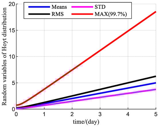
Figure 7.
The trend of the random variable characteristic number of Hoyt distributions over time ( = 0.001°/h).
6. Results of Simulation
For long-endurance inertial navigation systems, it is difficult to obtain a large number of test samples for verification. For now, the correctness of the above theoretical derivation will be verified through Monte Carlo simulation. The equivalent gyro bias is set to 0.001°/h, and 10,000 Monte Carlo experiments are conducted under static base conditions.
The probability density surface of radial error over time under static base conditions is shown in Figure 8, which is basically consistent with the Hoyt distribution probability density surface, but significantly different from the normal distribution with a symmetric form probability density curve, indicating that the Hoyt distribution is more suitable as a probability distribution model for the radial positioning error compared to the normal distribution.
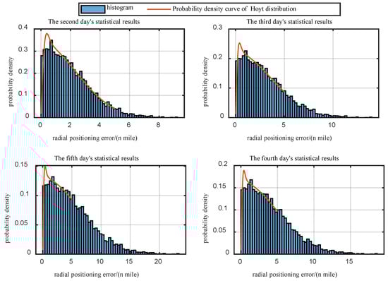
Figure 8.
Comparison of PDF and Hoyt distributions of radial positioning errors at different times under static base simulation conditions.
To further compare the differences in Max metrics calculated based on normal distribution and Hoyt distribution in accuracy evaluation, Table 1 presents the actual statistical values of the experimental results, as well as the prior values, estimated values, and estimated values calculated based on Hoyt distribution and normal distribution. The results of “Estimated value using prior information” are obtained by directly bringing the equivalent gyro zero bias ( = 0.001°/h) set in the simulation into Equation (38). The corresponding MEAN\STD\MAX is then obtained based on the proportionality between RMS and Mean\Std\Max. The results of “Estimated value using Hoyt distribution” require the estimation of the equivalent gyro zero bias using the method introduced in Section 4.3 after obtaining the radial positioning error data. The results of “Estimated value using Normal distribution” are obtained by using the mean of the sample plus three times the standard deviation of the sample to calculate the Max value.

Table 1.
Statistical values of experimental results and estimated values under different distribution conditions.
From the results in Table 1, it can be concluded that before conducting the experiment, the estimated radial positioning error statistic based solely on the prior information of the equivalent angular velocity has an error of no more than 0.7% in mean, standard deviation, and RMS compared to the actual statistical results, and an error of no more than 0.4% in Max. After obtaining the experimental results and estimating the statistical statistics of radial positioning error under the Hoyt distribution model assumption, the mean, standard deviation, and RMS errors do not exceed 0.13% compared to the actual statistical results, and the error of Max does not exceed 1%. However, under the assumption of a normal distribution model, the statistics of the estimated radial positioning error are compared with the actual statistical results (the mean, standard deviation, and RMS of the normal distribution are calculated using the same method as the actual values, so no comparison is made), and the error of Max exceeds 13%.
Figure 9 shows the cumulative probability distribution statistics of the results over time, the RMS and Max values estimated based on the prior information, the Hoyt distribution, and the normal distribution.
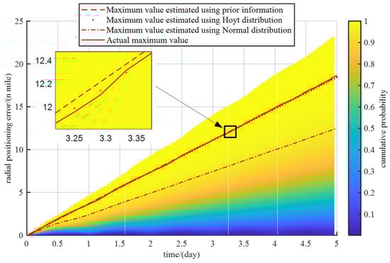
Figure 9.
The statistical results of cumulative probability distribution of radial positioning error and maximum value using different calculation methods.
7. Conclusions
As one of the critical indicators of long-inertial navigation, the radial positioning error of the inertial navigation systems has been extended to a normal distribution as the probability distribution model for accuracy test design. However, from the theoretical derivation and Monte Carlo simulation results in this paper, it can be seen that the Hoyt distribution is closer to the probability distribution of the radial positioning error of the inertial navigation systems; the parameters of the Hoyt distribution correspond to the primary error source of the inertial navigation systems (the equivalent gyro zero bias), and the probability distribution of the inertial navigation systems over time can be obtained from the radial positioning error data under multiple static base conditions. The theoretically derived probability distribution model of the static base error of the inertial navigation systems in this paper can be used as the a priori information on the probability distribution of the inertial navigation systems under the dynamic base condition to guide the design and analysis of the radial positioning accuracy test of the inertial navigation systems under the dynamic base condition.
Author Contributions
Y.H.: conceptualization, methodology, writing—reviewing and editing, investigation. H.B. and R.W.: supervision, resources, funding acquisition, visualization. R.W.: software, investigation. Z.W.: methodology. S.H.: methodology. All authors have read and agreed to the published version of the manuscript.
Funding
This research was funded by National Natural Science Foundation of China, grant number 41876222.
Data Availability Statement
The original contributions presented in this study are included in the article. Further inquiries can be directed to the corresponding author.
Conflicts of Interest
The authors declare no conflicts of interest. The funders had no role in the design of the study; in the collection, analyses, or interpretation of data; in the writing of the manuscript; or in the decision to publish the results.
References
- Li, D.; Yu, X.; Wei, G.; Yuan, B.; Gao, C.; Zhang, P.; Wang, G.; Luo, H. Development and Prospects of Long-Endurance Ring Laser Gyro Inertial Navigation System Technology. Acta Opt. Sin. 2023, 43, 112–126. [Google Scholar] [CrossRef]
- Zhao, K.; Hu, X.; Liu, B. Long-Endurance Fiber Optic Gyroscope INS for Ships and Its Development Trends. J. Chin. Inert. Technol. 2022, 30, 282–287. [Google Scholar] [CrossRef]
- Liu, W.R.; Li, D.C.; Li, M.C.; Wei, J.X.; Zhao, X.M. Prospect of High Precision Marine FOG Inertial Navigation Technology. Navig. Control 2022, 21, 241–249. [Google Scholar] [CrossRef]
- El-Sheimy, N.; Youssef, A. Inertial Sensors Technologies for Navigation Applications: State of the Art and Future Trends. Satell. Navig. 2020, 1, 2. [Google Scholar] [CrossRef]
- El-Diasty, M.; Pagiatakis, S. Calibration and Stochastic Modelling of Inertial Navigation Sensor Erros. J. Glob. Position. Syst. 2008, 7, 170–182. [Google Scholar] [CrossRef]
- Zheng, T.; Xu, A.; Xu, X.; Liu, M. Modeling and Compensation of Inertial Sensor Errors in Measurement Systems. Electronics 2023, 12, 2458. [Google Scholar] [CrossRef]
- Wang, B.; Ren, Q.; Deng, Z.; Fu, M. A Self-Calibration Method for Nonorthogonal Angles between Gimbals of Rotational Inertial Navigation System. IEEE Trans. Ind. Electron. 2015, 62, 2353–2362. [Google Scholar] [CrossRef]
- Li, D.; Wei, G.; Wang, L.; Luo, H.; Yu, X. An Efficient System-Level Calibration Method for a High-Precision RLG RINS Considering the G-Sensitive Misalignment. IEEE Trans. Ind. Electron. 2024, 71, 16823–16833. [Google Scholar] [CrossRef]
- Lyu, X.; Zhu, J.; Wang, J.; Dong, R.; Qian, S.; Hu, B. A Novel Method for Damping State Switching Based on Machine Learning of a Strapdown Inertial Navigation System. Electronics 2024, 13, 3439. [Google Scholar] [CrossRef]
- Liu, Y.; Yang, G.; Cai, Q.; Wang, L.; Wang, S. Design of External Damping Network and Discretization Algorithm for Long-Endurance Inertial Navigation System. In Proceedings of the 2020 7th International Conference on Information Science and Control Engineering (ICISCE), Changsha, China, 18–20 December 2020; pp. 498–502. [Google Scholar]
- Zhu, T.; Li, J.; Duan, K.; Sun, S. Study on the Robust Filter Method of SINS/DVL Integrated Navigation Systems in a Complex Underwater Environment. Sensors 2024, 24, 6596. [Google Scholar] [CrossRef] [PubMed]
- Gao, Z. Research on Space-Stable Inertial Navigation System; TsingHua University Press: Beijing, China, 2021; ISBN 978-7-302-58862-7. [Google Scholar]
- Nokia Bell Labs. Probability Functions for the Modulus and Angle of the Normal Complex Variate. Bell Syst. Tech. J. 1947, 26, 318–359. [Google Scholar] [CrossRef]
- Nakagami, M. The m-Distribution—A General Formula of Intensity Distribution of Rapid Fading. In Statistical Methods in Radio Wave Propagation; Hoffman, W.C., Ed.; Pergamon: Oxford, UK, 1960; pp. 3–36. ISBN 978-0-08-009306-2. [Google Scholar]
- Paris, J.F. Erratum for ‘Nakagami-q (Hoyt) Distribution Function with Applications’. Electron. Lett. 2009, 45, 432. [Google Scholar] [CrossRef]
- Paris, J.F. Nakagami-q (Hoyt) Distribution Function with Applications. Electron. Lett. 2009, 45, 210. [Google Scholar] [CrossRef]
- Simon, M.K.; Alouini, M.-S. Digital Communication over Fading Channels: A Unified Approach to Performance Analysis; Wiley series in telecommunications and signal processing; John Wiley & Sons: New York, NY, USA, 2000; ISBN 978-0-471-31779-1. [Google Scholar]
- Abramowitz, M.; Stegun, I.A. Handbook of Mathematical Functions with Formulas, Graphs, and Mathematical Tables, 9th ed.; Dover Press: New York, NY, USA, 1972. [Google Scholar]
- Wang, R.; Bian, H.; Liu, W. Analysis of Stochastic Errors Impact in SINS Based on RMSE. J. Nav. Univ. Eng. 2017, 29, 18–23+27. [Google Scholar] [CrossRef]
- Romero-Jerez, J.M.; Lopez-Martinez, F.J. A New Framework for the Performance Analysis of Wireless Communications Under Hoyt (Nakagami-q) Fading. IEEE Trans. Inf. Theory 2017, 63, 1693–1702. [Google Scholar] [CrossRef]
Disclaimer/Publisher’s Note: The statements, opinions and data contained in all publications are solely those of the individual author(s) and contributor(s) and not of MDPI and/or the editor(s). MDPI and/or the editor(s) disclaim responsibility for any injury to people or property resulting from any ideas, methods, instructions or products referred to in the content. |
© 2024 by the authors. Licensee MDPI, Basel, Switzerland. This article is an open access article distributed under the terms and conditions of the Creative Commons Attribution (CC BY) license (https://creativecommons.org/licenses/by/4.0/).