

Accelerating Die Bond Quality Detection Using Lightweight Architecture DSGβSI-Yolov7-Tiny


Abstract
1. Introduction
2. Related Work
2.1. Literature Review
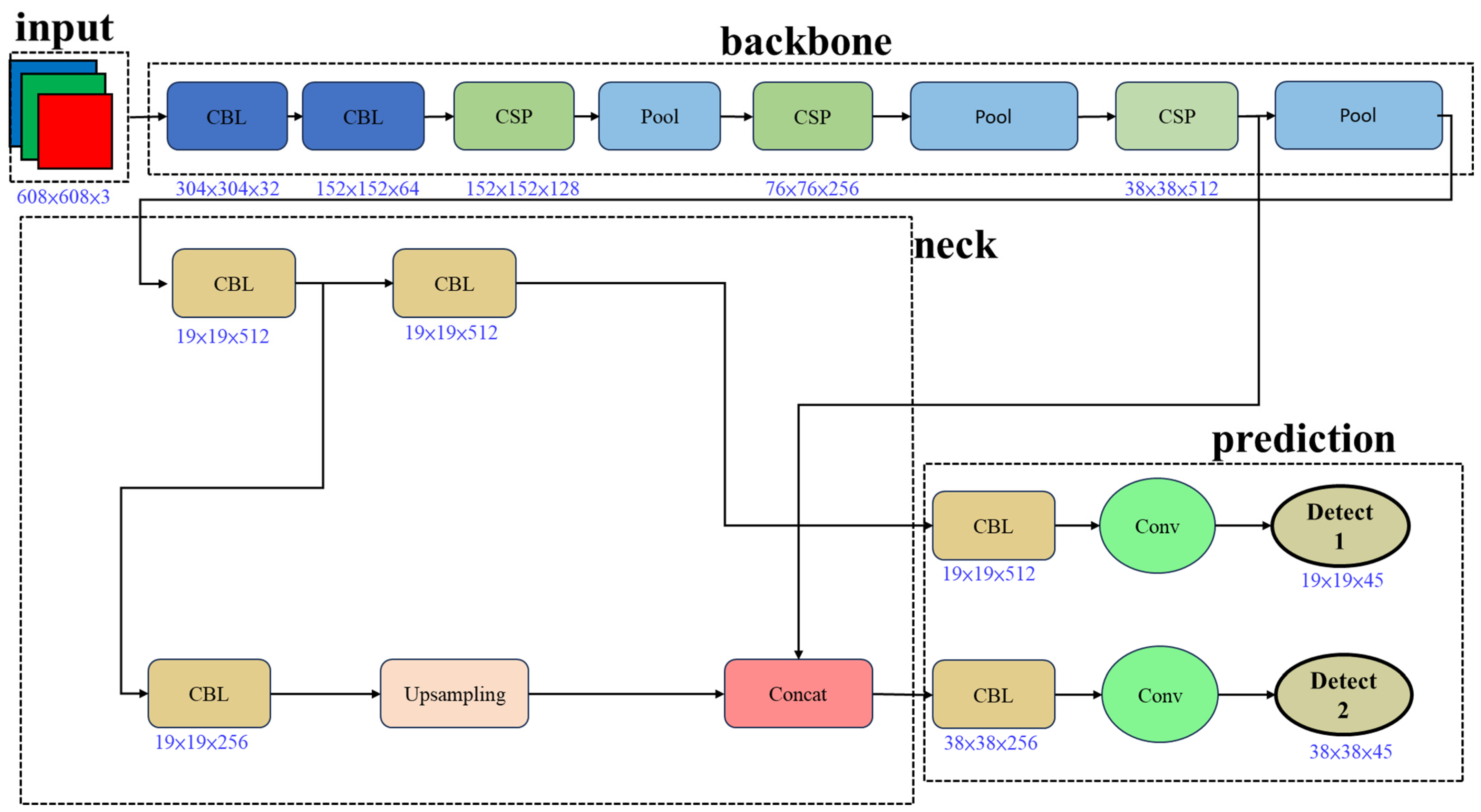
2.2. The Yolov4-Tiny Model
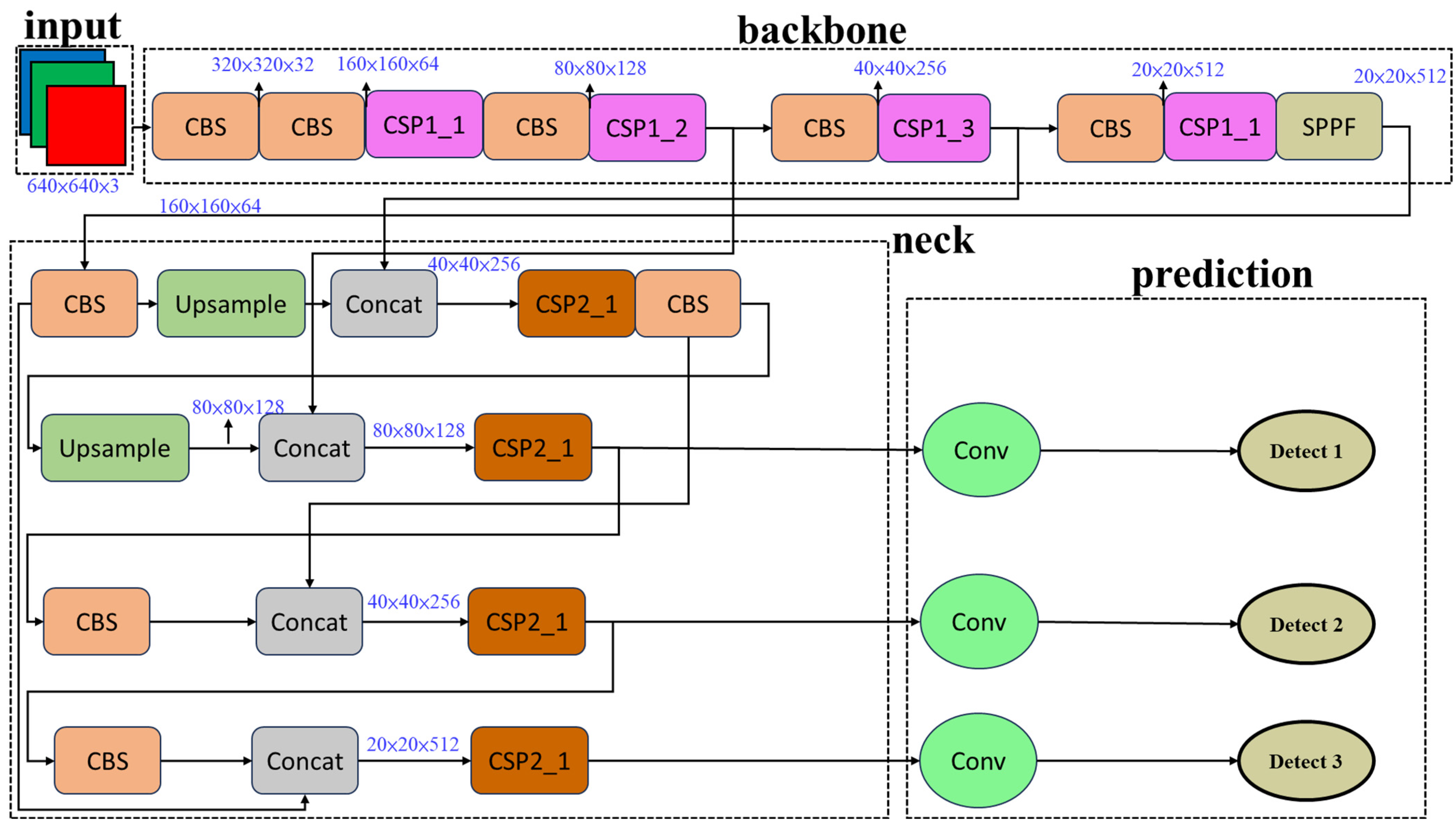
2.3. The Yolov5n Model
2.4. The Yolov7 Model
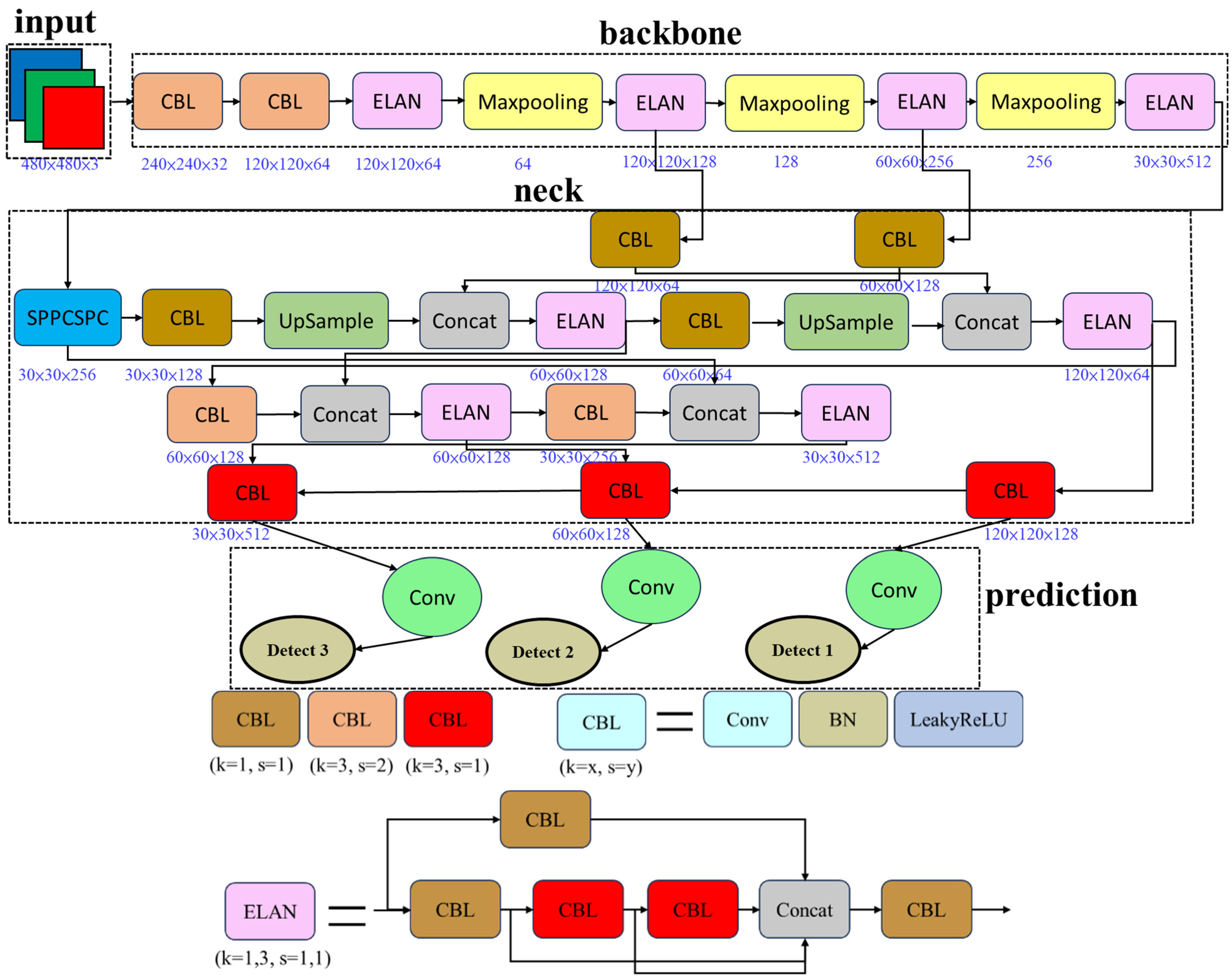
2.5. The Yolov7-Tiny Model
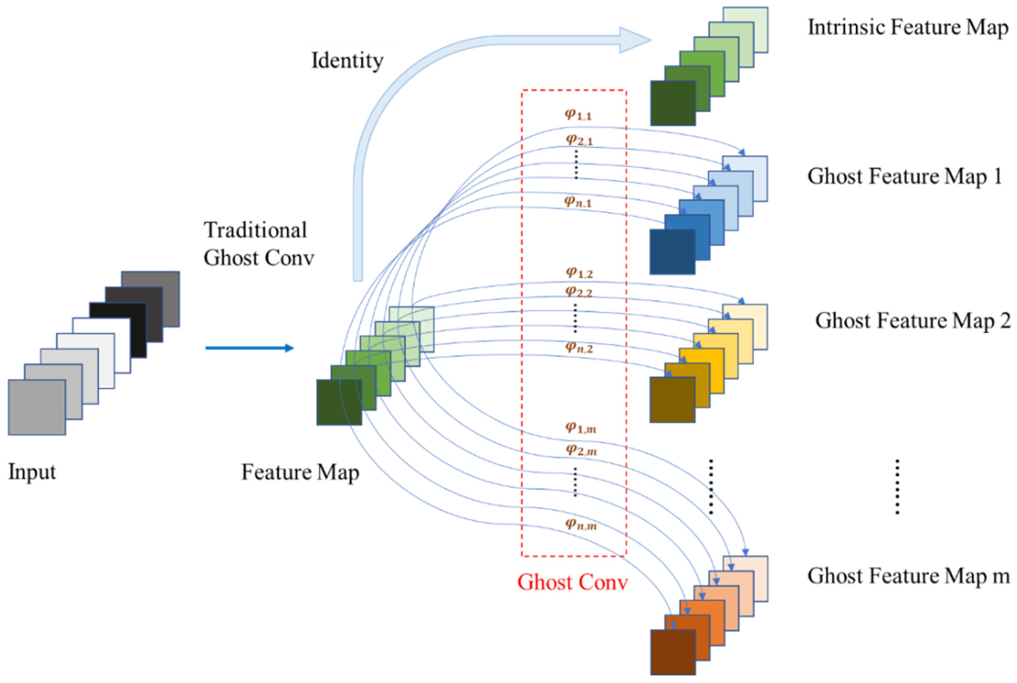
2.6. The DSG-Yolov7 Model
3. Methods
3.1. Data Collection and Preprocessing
3.2. Recognition Data
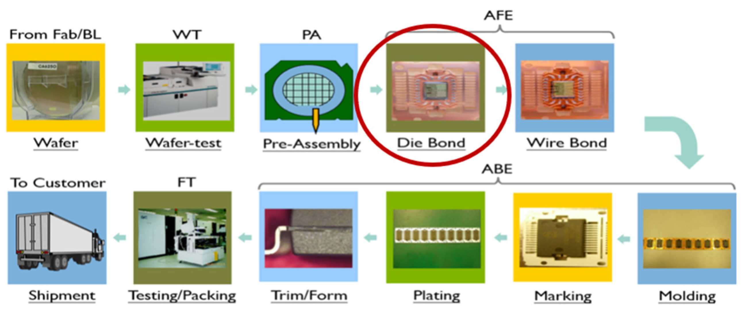
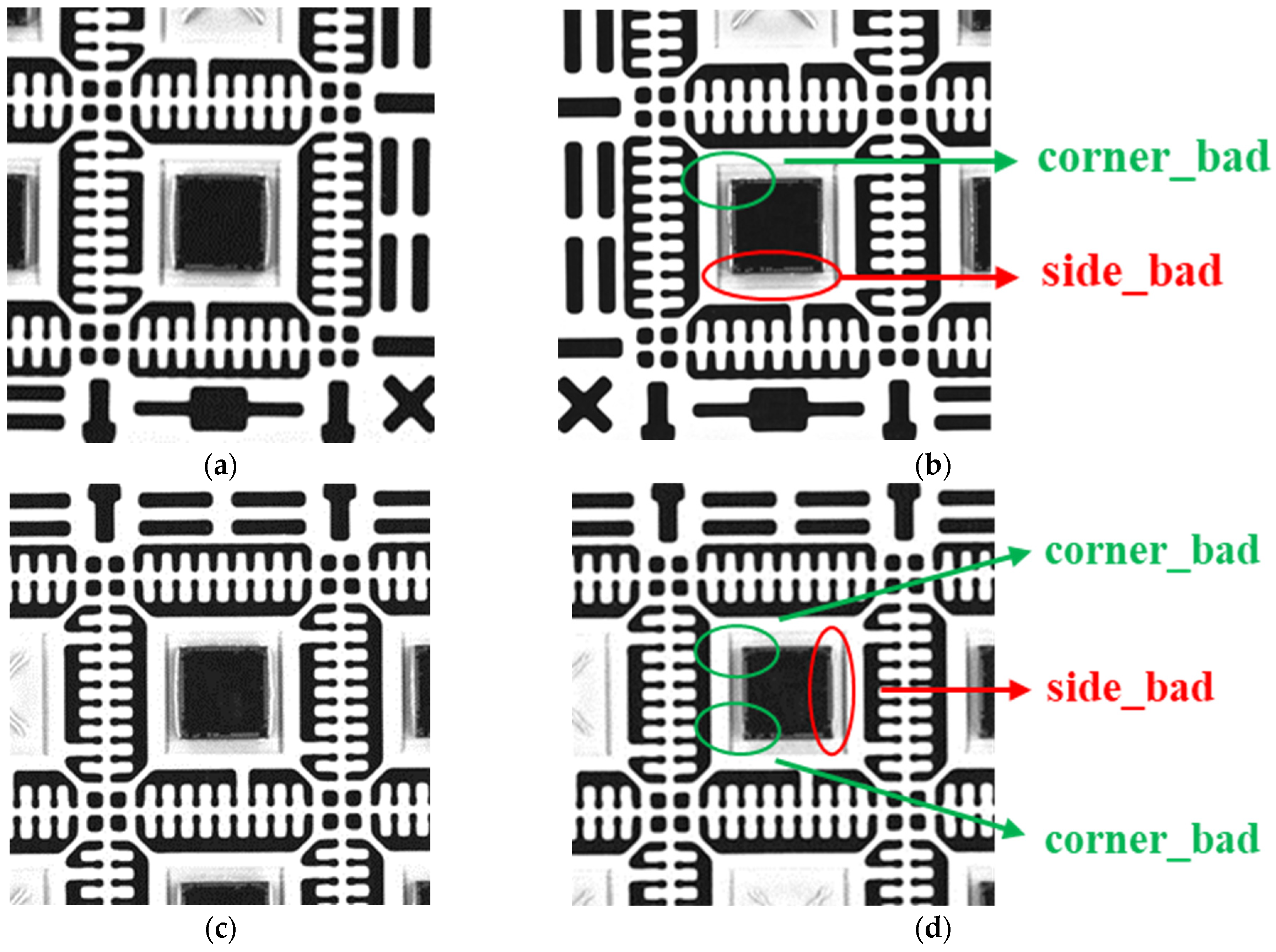
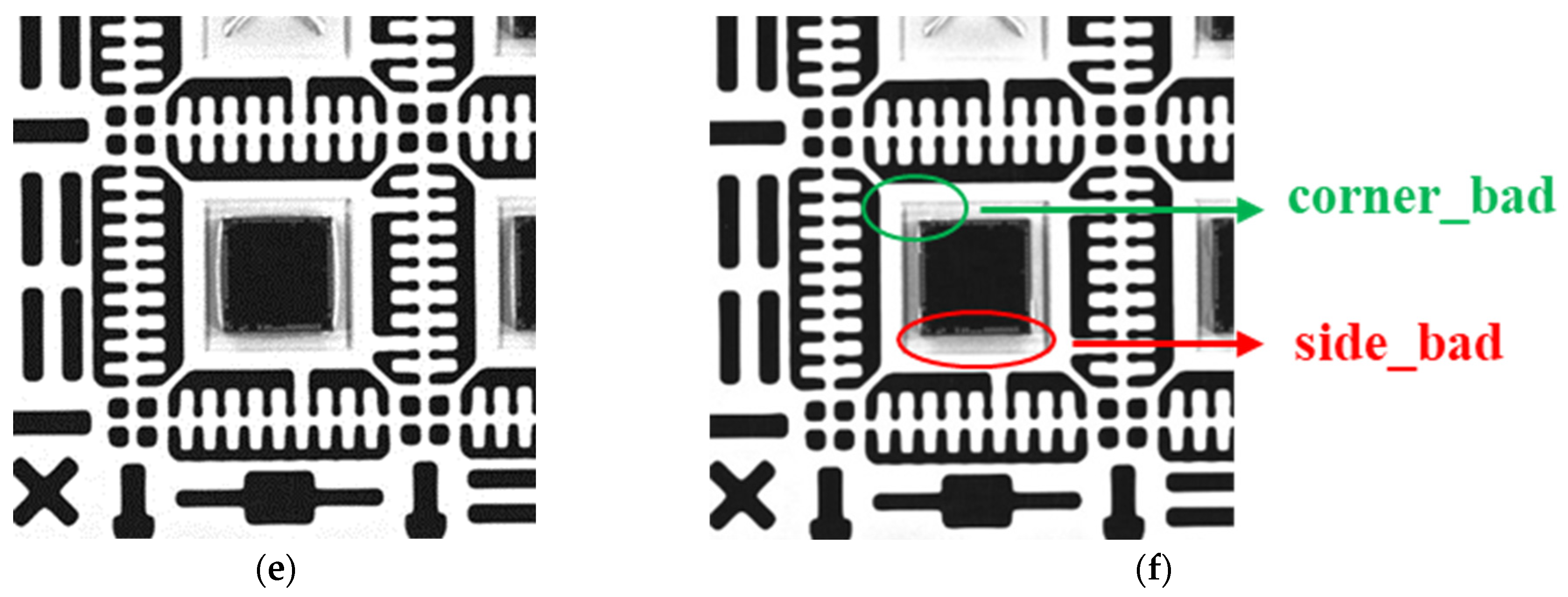
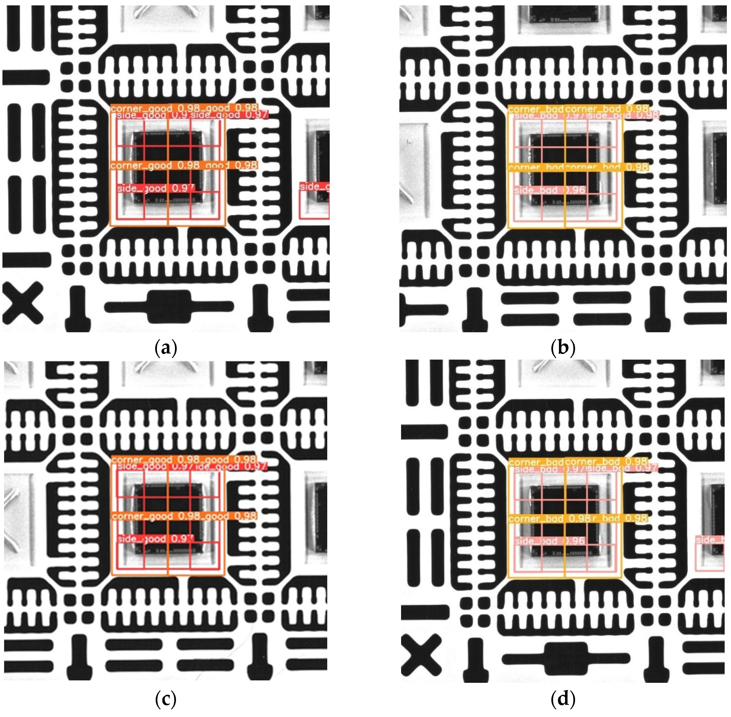
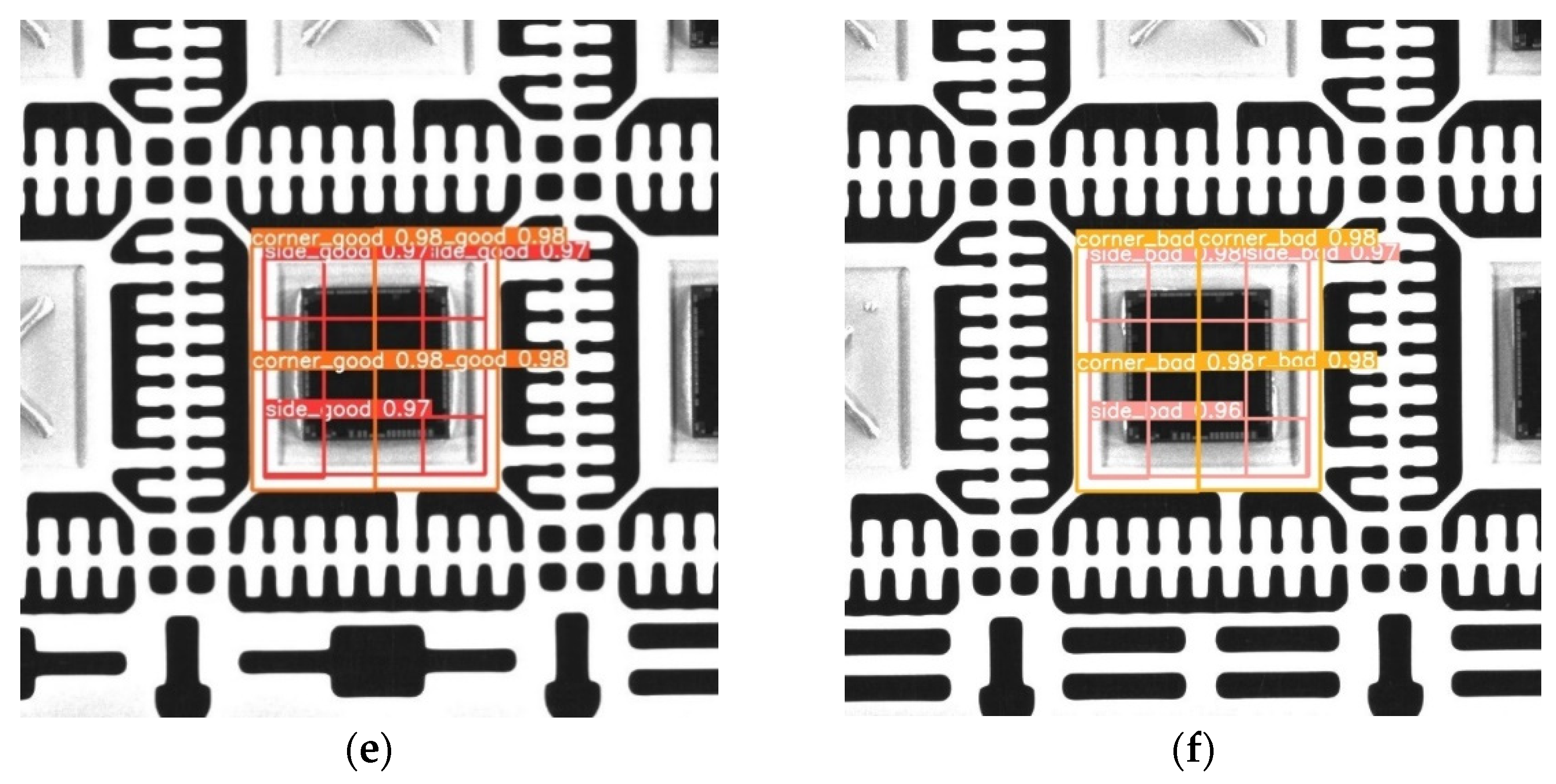
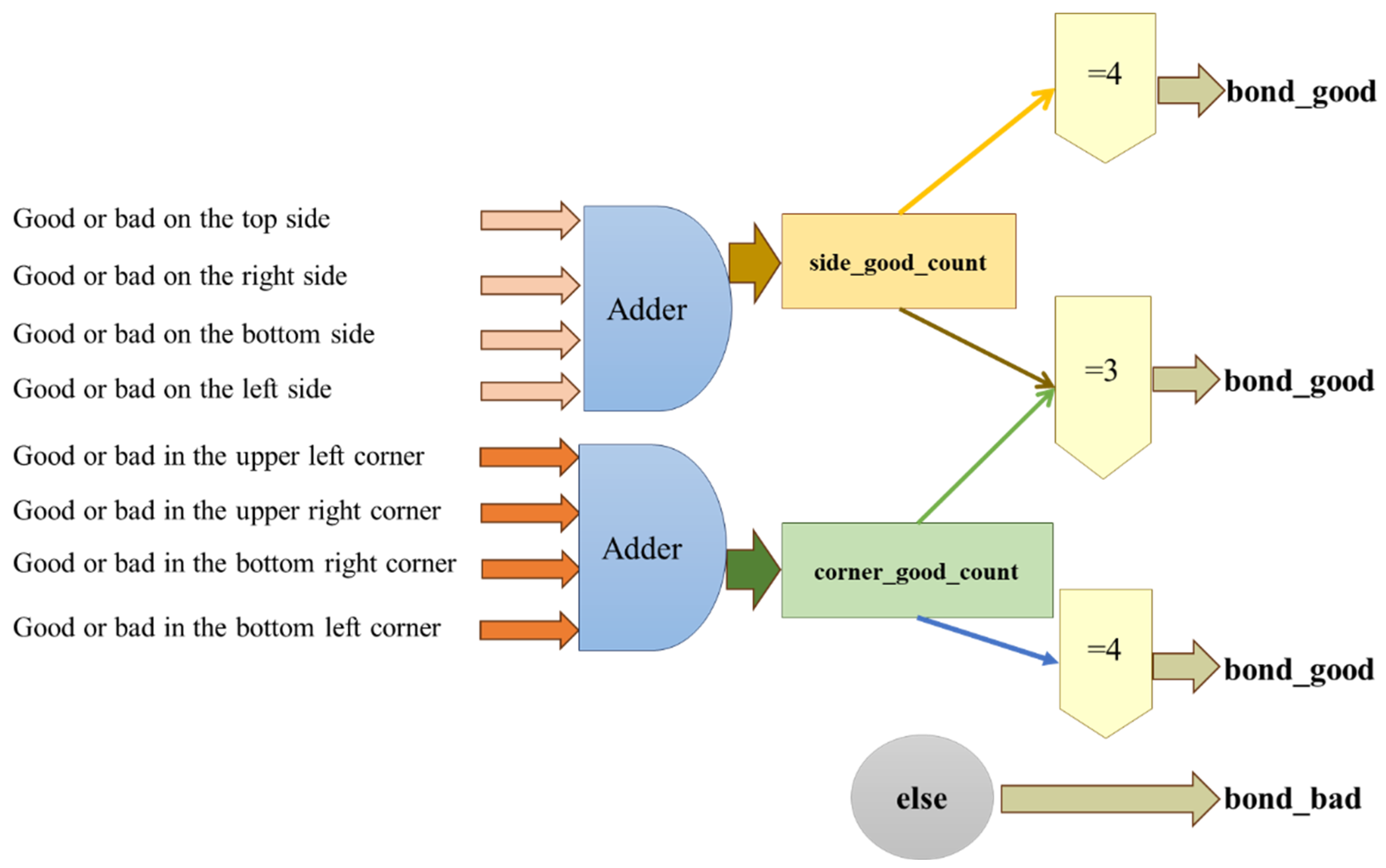
3.3. Judgment of Detection Results and Types of Die Bonding
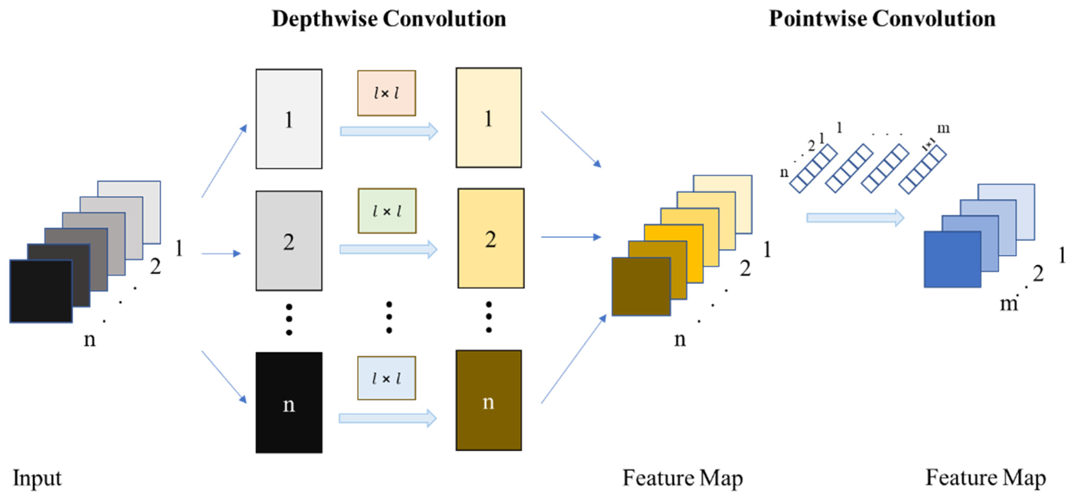
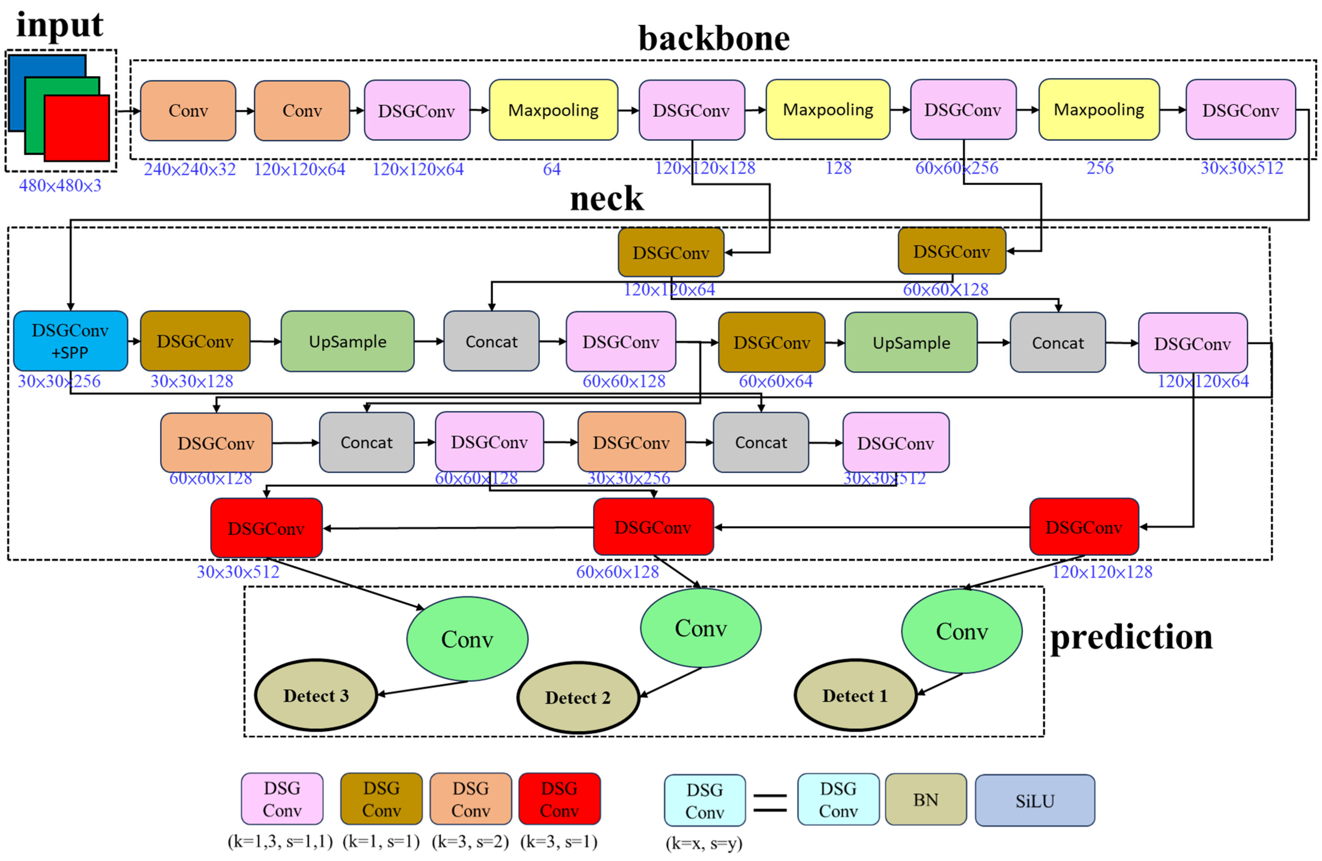
3.4. Model Improvement
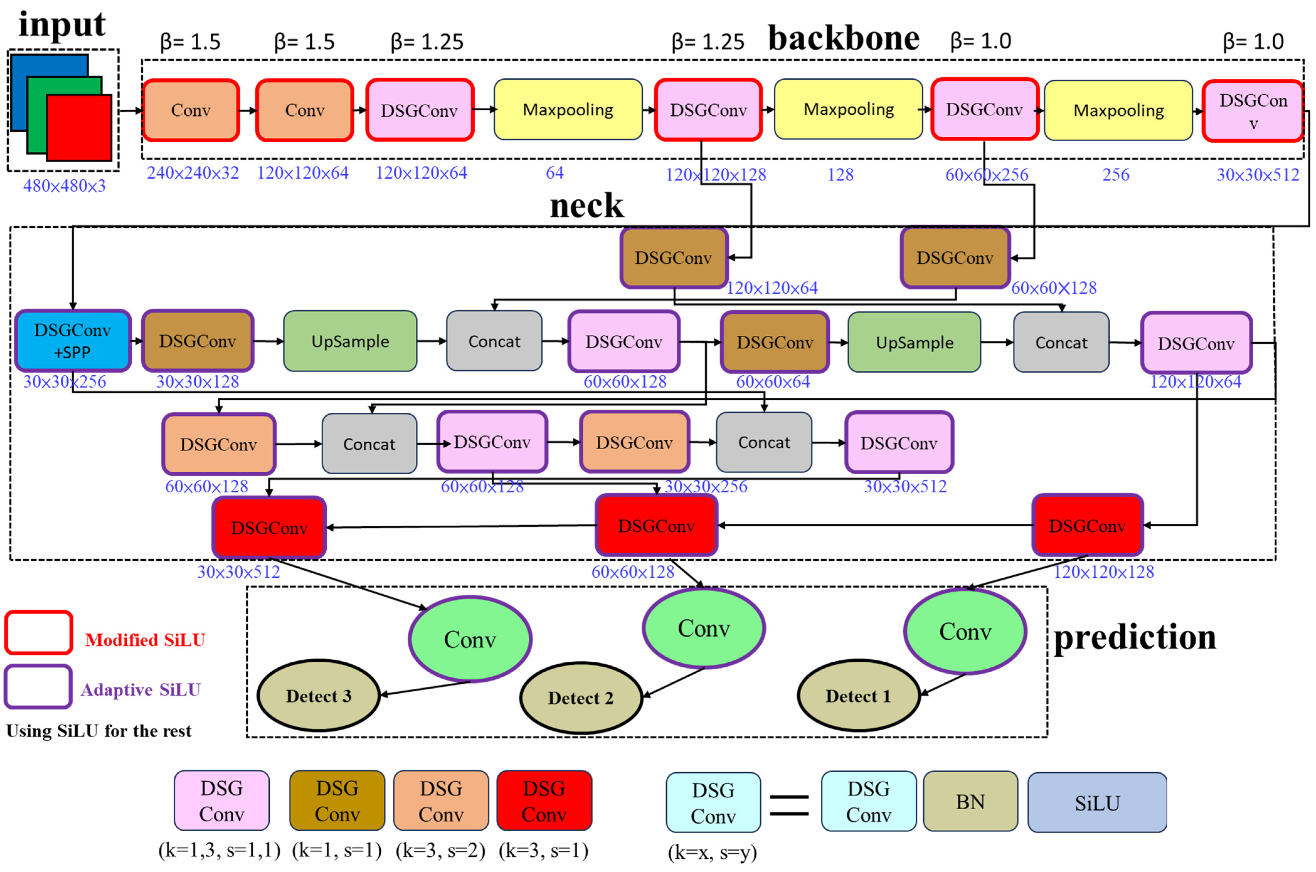
3.5. Model Enhancement
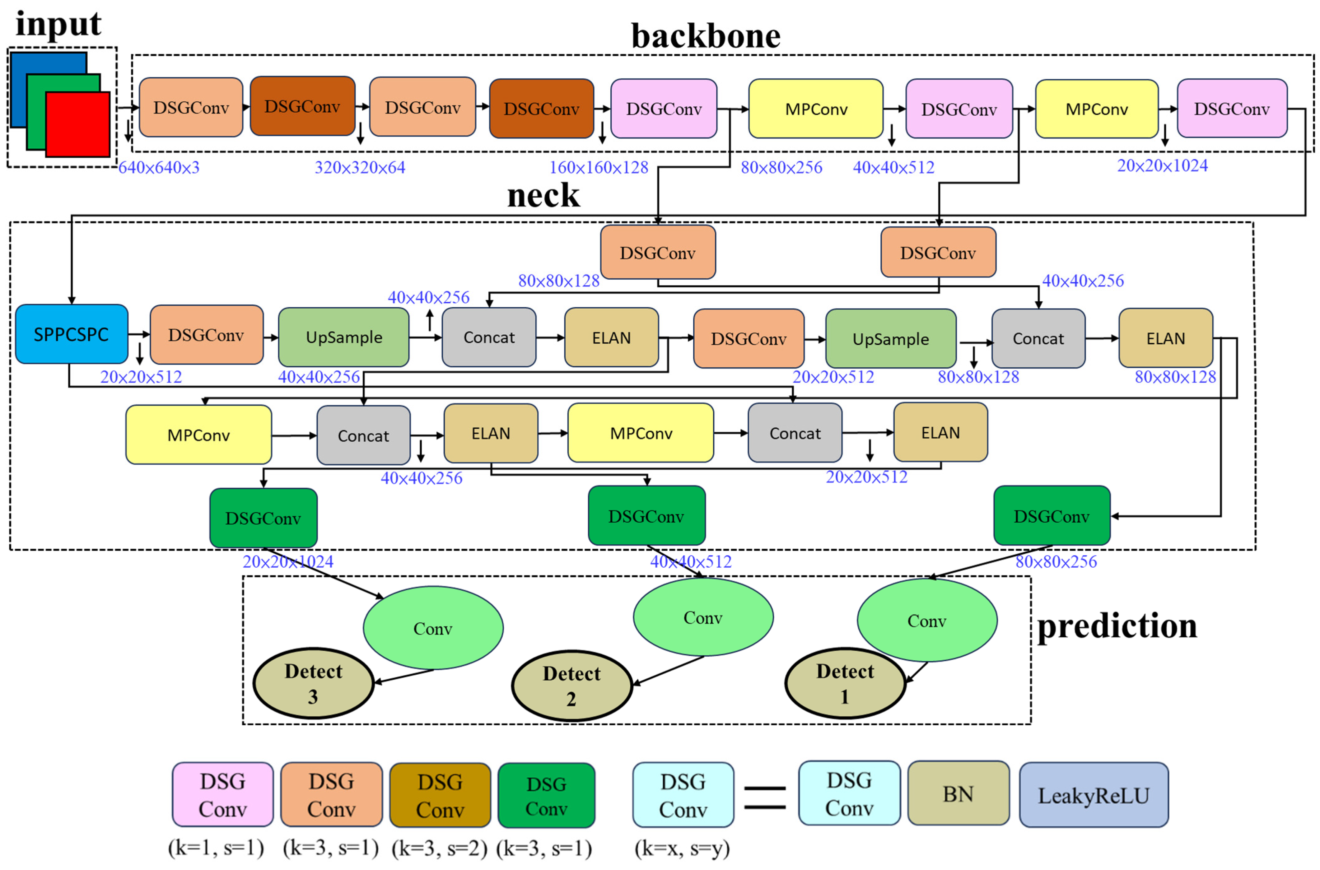
3.6. Build a Model
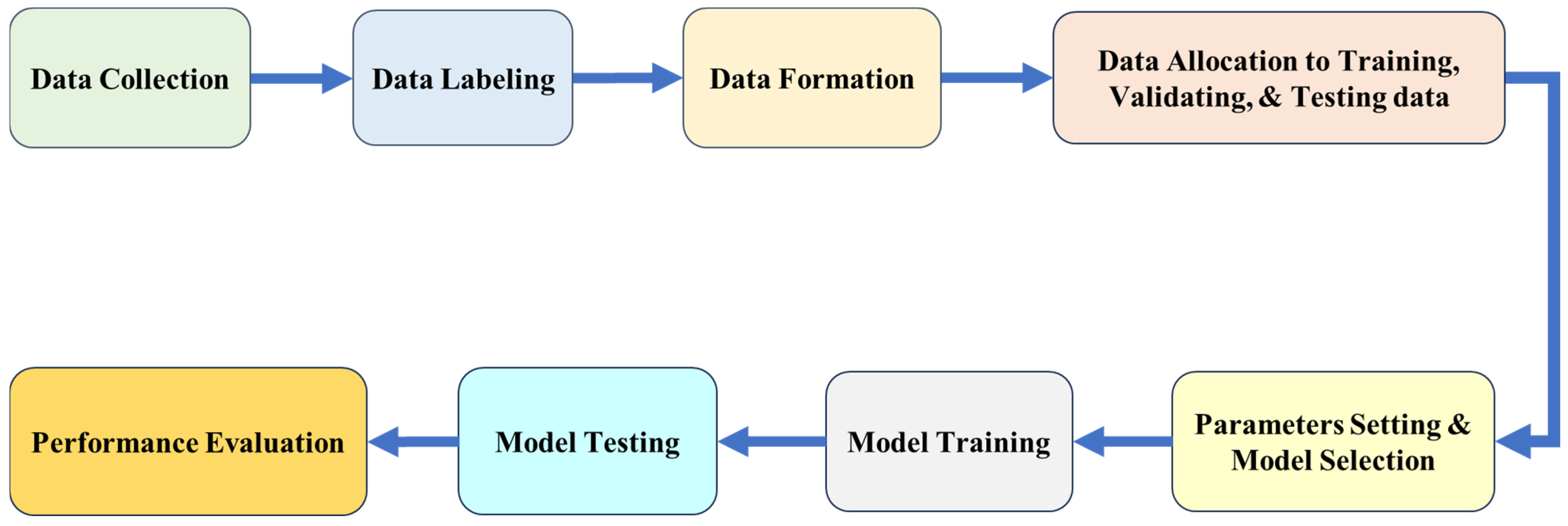
3.7. The Workflow of the System
4. Experimental Results and Discussion
4.1. Experimental Environment
4.2. Data Collection and Model Evaluation
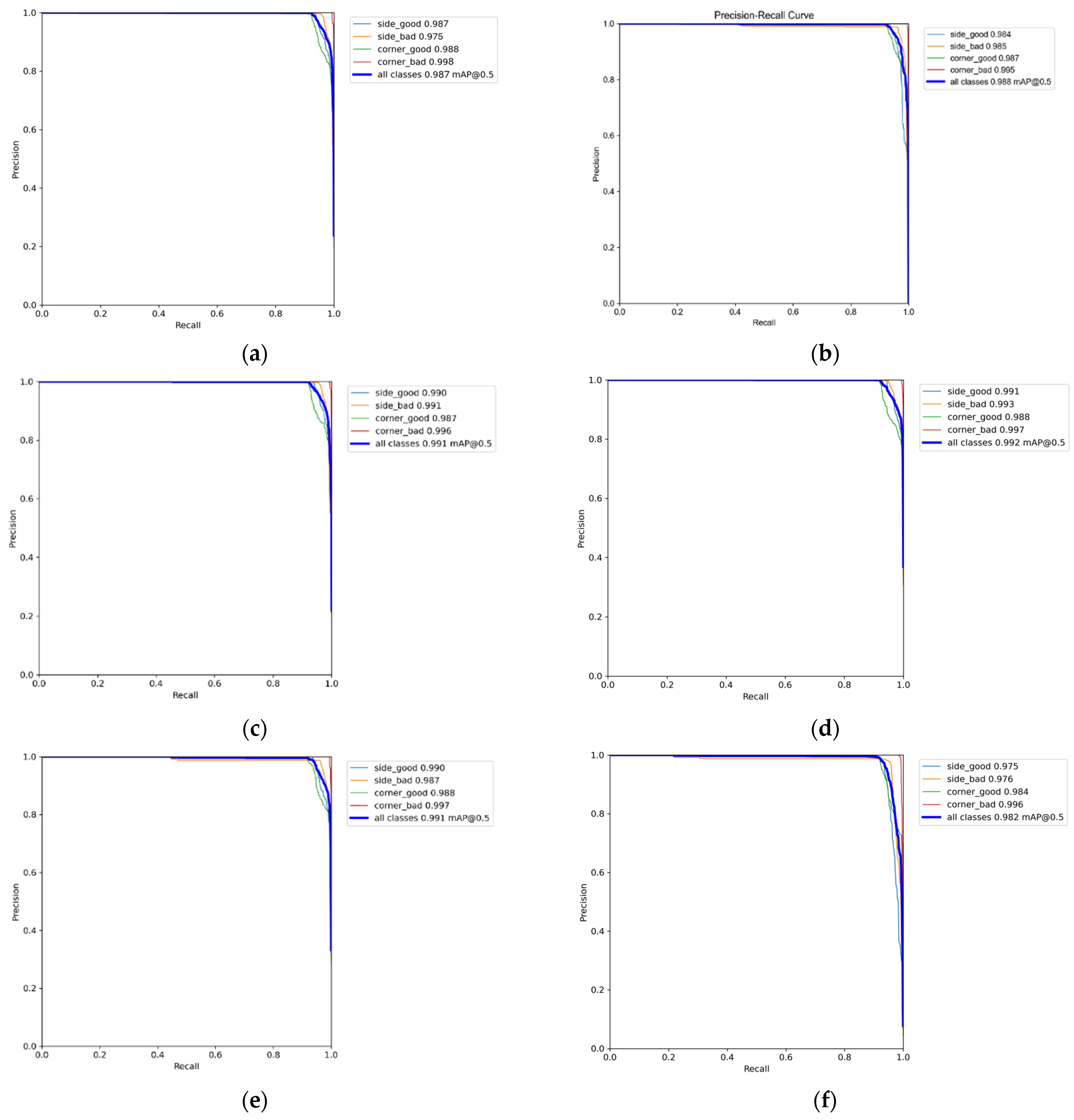
4.3. Experimental Results
4.4. Performance Evaluation
4.5. Discussion
5. Conclusions
Author Contributions
Funding
Data Availability Statement
Conflicts of Interest
References
- Chen, M.-F.; Chen, C.-W.; Chen, C.-Y.; Hwang, C.-H.; Hwang, L.-Y. An AOI system development for inspecting defects on 6 surfaces of chips. In Proceedings of the 2016 IEEE International Instrumentation and Measurement Technology Conference Proceedings, Taipei, Taiwan, 23–26 May 2016; pp. 1–6. [Google Scholar]
- Yang, Y.; Wang, X. An improved YOLOv7-tiny-based lightweight network for the identification of fish species. In Proceedings of the 2023 5th International Conference on Robotics and Computer Vision (ICRCV), Nanjing, China, 15–17 September 2023; pp. 188–192. [Google Scholar]
- Chang, B.R.; Tsai, H.-F.; Chang, F.-Y. Applying advanced lightweight architecture DSGSE-Yolov5 to rapid chip contour detection. Electronics 2024, 13, 10. [Google Scholar] [CrossRef]
- Chang, B.R.; Tsai, H.-F.; Chang, F.-Y. Boosting the response of object detection and steering angle prediction for self-driving control. Electronics 2023, 12, 4281. [Google Scholar] [CrossRef]
- Li, C.; Tan, G.; Wu, C.; Li, M. YOLOv7-VD: An algorithm for vehicle detection in complex environments. In Proceedings of the 2023 4th International Conference on Computer, Big Data and Artificial Intelligence (ICCBD+AI), Guiyang, China, 15–17 December 2023; pp. 743–747. [Google Scholar]
- Alam, L.; Kehtarnavaz, N. A survey of detection methods for die attachment and wire bonding defects in integrated circuit manufacturing. IEEE Access 2022, 10, 83826–83840. [Google Scholar] [CrossRef]
- Phan, Q.-H.; Nguyen, V.-T.; Lien, C.-H.; Duong, T.-P.; Hou, M.T.-K.; Le, N.-B. Classification of tomato fruit using YOLOv5 and convolutional neural network models. Plants 2023, 12, 790. [Google Scholar] [CrossRef] [PubMed]
- Hsiao, S.-F.; Tsai, B.-C. Efficient computation of depthwise separable convolution in MobileNet deep neural network models. In Proceedings of the 2021 IEEE International Conference on Consumer Electronics-Taiwan (ICCE-TW), Penghu, Taiwan, 15–17 September 2021; pp. 1–2. [Google Scholar]
- Howard, A.G.; Zhu, M.; Chen, B.; Kalenichenko, D.; Wang, W.; Weyand, T.; Andreetto, M.; Adam, H. MobileNets: Efficient convolutional neural networks for mobile vision applications. arXiv 2017, arXiv:1704.04861. [Google Scholar]
- Wang, T.; Ray, N. Compact Depth-Wise Separable Precise Network for Depth Completion. IEEE Access 2023, 11, 72679–72688. [Google Scholar] [CrossRef]
- Zhang, Y.; Cai, W.; Fan, S.; Song, R.; Jin, J. Object detection based on YOLOv5 and GhostNet for orchard pests. Information 2022, 13, 548. [Google Scholar] [CrossRef]
- Sun, D.; Zhang, L.; Wang, J.; Liu, X.; Wang, Z.; Hui, Z.; Wang, J. Efficient and accurate detection of herd pigs based on Ghost-YOLOv7-SIoU. Neural Comput. Appl. 2024, 36, 2339–2352. [Google Scholar] [CrossRef]
- Lang, C.; Yu, X.; Rong, X. LSDNet: A lightweight ship detection network with improved YOLOv7. J. Real-Time Image Process. 2024, 21, 60. [Google Scholar] [CrossRef]
- Wu, Y.; Tang, Y.; Yang, T. An improved nighttime people and vehicle detection algorithm based on YOLOv7. In Proceedings of the 2023 3rd International Conference on Neural Networks, Information and Communication Engineering (NNICE), Guangzhou, China, 24–26 February 2023; pp. 266–270. [Google Scholar]
- Shafiee Sarvestani, A.; Zhou, W.; Wang, Z. Perceptual Crack Detection for Rendered 3D Textured Meshes. arXiv 2024, arXiv:2405.06143. [Google Scholar]
- Song, X.; Chen, L.; Zhang, L.; Luo, J. Optimal proposal learning for deployable end-to-end pedestrian detection. In Proceedings of the IEEE/CVF Conference on Computer Vision and Pattern Recognition (CVPR), Vancouver, BC, Canada, 17–24 June 2023; pp. 3250–3260. [Google Scholar]
- Han, K.; Wang, Y.; Tian, Q.; Guo, J.; Xu, C.; Xu, C. GhostNet: More features from cheap operations. In Proceedings of the IEEE/CVF Conference on Computer Vision and Pattern Recognition, Seattle, WA, USA, 13–19 June 2020; pp. 1580–1589. [Google Scholar]
- Madhuri, P.; Akhter, N.; Raj, A.B. Digital implementation of depthwise separable convolution network for AI applications. In Proceedings of the 2023 IEEE Pune Section International Conference (PuneCon), Pune, India, 14–16 December 2023; pp. 1–5. [Google Scholar]
- Lee, J.H.; Kong, J.; Munir, A. Arithmetic coding-based 5-bit weight encoding and hardware decoder for CNN inference in edge devices. IEEE Access 2021, 9, 166736–166749. [Google Scholar] [CrossRef]
- Mou, C.; Zhu, C.; Liu, T.; Cui, X. A novel efficient wildlife detecting method with lightweight deployment on UAVs based on YOLOv7. IET Image Process. 2024, 18, 1296–1314. [Google Scholar] [CrossRef]
- Li, B.; Liu, L.; Wang, S.; Liu, X. Research on object detection algorithm based on improved YOLOv7. In Proceedings of the 9th International Conference on Computer and Communication (ICCC), Chengdu, China, 8–11 December 2023; pp. 1724–1727. [Google Scholar]
- Sun, H.-R.; Shi, B.-J.; Zhou, Y.-T.; Chen, J.-H.; Hu, Y.-L. A Smoke Detection Algorithm Based on Improved YOLO v7 Lightweight Model for UAV Optical Sensors. IEEE Sens. J. 2024, 24, 26136–26147. [Google Scholar] [CrossRef]
- Sai, T.A.; Lee, H. Weight initialization on neural network for neuro pid controller-case study. In Proceedings of the 2018 International Conference on Information and Communication Technology Robotics (ICT-ROBOT), Busan, Republic of Korea, 6–8 September 2018; pp. 1–4. [Google Scholar]
- Wong, K.; Dornberger, R.; Hanne, T. An analysis of weight initialization methods in connection with different activation functions for feedforward neural networks. Evol. Intell. 2024, 17, 2081–2089. [Google Scholar] [CrossRef]
- Ioffe, S.; Szegedy, C. Batch normalization: Accelerating deep network training by reducing internal covariate shift. arXiv 2015, arXiv:1502.03167. [Google Scholar]


| s | 0 | 1 | 2 | 3 | 4 | 5 | 6 | 7 | 8 | 9 | A | B | C | D | E | F | |
|---|---|---|---|---|---|---|---|---|---|---|---|---|---|---|---|---|---|
| c | |||||||||||||||||
| 0 | b | b | b | b | b | b | b | g | b | b | b | g | b | g | g | g | |
| 1 | b | b | b | b | b | b | b | g | b | b | b | g | b | g | g | g | |
| 2 | b | b | b | b | b | b | b | g | b | b | b | g | b | g | g | g | |
| 3 | b | b | b | b | b | b | b | g | b | b | b | g | b | g | g | g | |
| 4 | b | b | b | b | b | b | b | g | b | b | b | g | b | g | g | g | |
| 5 | b | b | b | b | b | b | b | g | b | b | b | g | b | g | g | g | |
| 6 | b | b | b | b | b | b | b | g | b | b | b | g | b | g | g | g | |
| 7 | g | g | g | g | g | g | g | g | g | g | g | g | g | g | g | g | |
| 8 | b | b | b | b | b | b | b | g | b | b | b | g | b | g | g | g | |
| 9 | b | b | b | b | b | b | b | g | b | b | b | g | b | g | g | g | |
| A | b | b | b | b | b | b | b | g | b | b | b | g | b | g | g | g | |
| B | g | g | g | g | g | g | g | g | g | g | g | g | g | g | g | g | |
| C | b | b | b | b | b | b | b | g | b | b | b | g | b | g | g | g | |
| D | g | g | g | g | g | g | g | g | g | g | g | g | g | g | g | g | |
| E | g | g | g | g | g | g | g | g | g | g | g | g | g | g | g | g | |
| F | g | g | g | g | g | g | g | g | g | g | g | g | g | g | g | g | |
| Model | Hyperparameters |
|---|---|
| Yolov4-tiny | ep = 120, bs = 16, is = 1024 × 1024, op = SGD, act = Leaky ReLU, Sigmoid, tc = |
| Yolov5n | ep = 120, bs = 16, is = 1024 × 1024, op = Adam, act = SiLU, Sigmoid, tc = |
| Yolov7 | ep = 120, bs = 16, is = 1024 × 1024, op = AdamW, act = Leaky ReLU, Sigmoid, tc = |
| Yolov7-tiny | ep = 120, bs= 16, is = 1024 × 1024, op = AdamW, act = Leaky ReLU, Sigmoid, tc = |
| DSG-Yolov7 | ep = 120, bs= 16, is = 1024 × 1024, op = AdamW, act = Leaky ReLU, Sigmoid, tc = |
| DSG-Yolov7-tiny | ep = 120, bs= 16, is = 1024 × 1024, op = AdamW, act = Leaky ReLU, Sigmoid, tc = |
| DSGSI-Yolov7-tiny | ep = 120, bs= 16, is = 1024 × 1024, op = AdamW, act = SiLU, Sigmoid, tc = |
| DSGβSI-Yolov7-tiny | ep = 120, bs= 16, is = 1024 × 1024, op = AdamW, act = ModifiedSiLU, AdaptiveSiLU, SiLU, Sigmoid, tc = |
| Resource | Workstation |
|---|---|
| GPU | NVIDIA GeForce RTX 4070 Ti |
| CPU | Intel(R) Xeon(R) W-2223 CPU @ 3.60 GHz |
| Memory | 32 GB |
| Storage | 1 TB × 1 (HDD) |
| Jetson Nano | NVIDIA Maxwell™ architecture with 128 NVIDIA CUDA® cores |
| Software | Version |
|---|---|
| LabelImg | 1.8 |
| Anaconda® Individual Edition | 4.9.2 |
| Jupyter Notebook | 6.1.4 |
| TensorFlow | v2.14.0 |
| PyTorch | 1.6 |
| Python | 3.6.9 |
| Phase | Yolov4-Tiny | Yolov5n | Yolov7 | Yolov7-Tiny | DSG-Yolov7 | DSG-Yolov7-Tiny | DSGSI-Yolov7-Tiny | DSGβSI-Yolov7-Tiny |
|---|---|---|---|---|---|---|---|---|
| Training (h) | 30.1 | 14.9 | 58.8 | 46.9 | 56.4 | 3.6 | 3.6 | 4.1 |
| Inference (ms) | 25.1 | 18.6 | 19.3 | 18.2 | 16.3 | 5.4 | 5.7 | 5.2 |
| Feature | Yolov4-Tiny | Yolov5n | Yolov7 | Yolov7-Tiny | DSG-Yolov7 | DSG-Yolov7-Tiny | DSGSI-Yolov7-Tiny | DSGβSI-Yolov7-Tiny |
|---|---|---|---|---|---|---|---|---|
| Parameter (#) | 6,056,610 | 1,764,577 | 60,231,067 | 36,497,954 | 22,363,042 | 605,242 | 745,378 | 743,829 |
| Flop (Gflops) | 14.0 | 4.1 | 13.2 | 103.2 | 61.3 | 1.6 | 1.9 | 1.8 |
| Metric | Yolov4-Tiny | Yolov5n | Yolov7 | Yolov7-Tiny | DSG-Yolov7 | DSG-Yolov7-Tiny | DSGSI-Yolov7-Tiny | DSGβSI-Yolov7-Tiny |
|---|---|---|---|---|---|---|---|---|
| FPS | 39.8 | 53.8 | 51.8 | 54.9 | 61.3 | 185.2 | 175.4 | 192.3 |
| Precision | 98.5 | 98.8 | 99.0 | 99.1 | 99.1 | 98.2 | 98.6 | 99.1 |
| Recall | 95.2 | 95.1 | 95.2 | 95.0 | 95.3 | 95.1 | 95.3 | 95.4 |
| F1-score | 0.96 | 0.97 | 0.97 | 0.97 | 0.97 | 0.97 | 0.97 | 0.97 |
| Accuracy | 98.7 | 98.9 | 98.9 | 98.5 | 99.0 | 98.0 | 98.5 | 98.5 |
Disclaimer/Publisher’s Note: The statements, opinions and data contained in all publications are solely those of the individual author(s) and contributor(s) and not of MDPI and/or the editor(s). MDPI and/or the editor(s) disclaim responsibility for any injury to people or property resulting from any ideas, methods, instructions or products referred to in the content. |
© 2024 by the authors. Licensee MDPI, Basel, Switzerland. This article is an open access article distributed under the terms and conditions of the Creative Commons Attribution (CC BY) license (https://creativecommons.org/licenses/by/4.0/).
Share and Cite
Chang, B.R.; Tsai, H.-F.; Chang, W.-S. Accelerating Die Bond Quality Detection Using Lightweight Architecture DSGβSI-Yolov7-Tiny. Electronics 2024, 13, 4573. https://doi.org/10.3390/electronics13224573
Chang BR, Tsai H-F, Chang W-S. Accelerating Die Bond Quality Detection Using Lightweight Architecture DSGβSI-Yolov7-Tiny. Electronics. 2024; 13(22):4573. https://doi.org/10.3390/electronics13224573
Chicago/Turabian StyleChang, Bao Rong, Hsiu-Fen Tsai, and Wei-Shun Chang. 2024. "Accelerating Die Bond Quality Detection Using Lightweight Architecture DSGβSI-Yolov7-Tiny" Electronics 13, no. 22: 4573. https://doi.org/10.3390/electronics13224573
APA StyleChang, B. R., Tsai, H.-F., & Chang, W.-S. (2024). Accelerating Die Bond Quality Detection Using Lightweight Architecture DSGβSI-Yolov7-Tiny. Electronics, 13(22), 4573. https://doi.org/10.3390/electronics13224573