Abstract
This paper introduces a preprocessing and feature selection technique for maritime target estimation. Given the distinct challenges of the maritime environment and the use of multiple sensors, we propose a target estimation model designed to achieve high accuracy while minimizing computational costs through suitable data preprocessing and feature selection. The experimental results demonstrate excellent performance, with the mean square error (MSE) reduced by about 99%. This approach is expected to enhance vessel tracking in situations where vessel estimation sensors, such as the automatic identification system (AIS), are disabled. By enabling reliable vessel tracking, this technique can aid in the detection of illegal vessels.
1. Introduction
The manipulation of vessel-tracking devices has emerged as a serious maritime management task worldwide. According to recent analyses [1,2,3,4], vessels around the world have been found to frequently turn off satellite tracking devices arbitrarily. This is presumed to be closely related to illegal, unreported, and unregulated (IUU) operations. Surprisingly, in vessel tracking, there are also ’hot spots’ in which tracking devices are turned off. These areas are mainly concentrated at the borders of exclusive economic zones (EEZs) or in international waters, suggesting the possibility of illegal fishing. In this situation, illegal operation monitoring using the existing vessel automatic identification system (AIS) is limited because accurately tracking the location or activity of the vessel is difficult when the AIS signal is blocked or manipulated. To overcome the limitations of existing vessel-tracking systems such as AIS, this study proposes a new model that can support maritime tracking when vessels are uncooperative. To this end, we collected datasets through maritime environment simulations for a combination of sensors with different characteristics including acoustic sensors, magnetic field sensors, and depth sensors. This study explores various preprocessing techniques to identify the most suitable approach for the experimental data, proposing a feature selection method to identify essential sensors for target tracking. Given the challenges of the marine environment and the use of multiple sensors, it is crucial to develop a model that demonstrates minimal error with limited resources. Thus, the proposed feature selection method is implemented in two stages. First, the sensor stability stage assesses the reliability of each sensor’s input values. Sensors with low reliability are eliminated at this stage, reducing the complexity of the subsequent target relevance stage and minimizing exceptional cases. In the target relevance stage, the sensors most essential for target tracking are selected. The proposed approach significantly reduces mean square error (MSE), resulting in approximately 99% improvement in performance. This study is expected to considerably support illegal fishing monitoring. Its impact could extend to domains beyond the marine environment by enabling effective target estimation even in situations where vessel estimation sensors such as AIS do not work, thereby enforcing international maritime law and protection of marine ecosystems.
The contributions of this study are summarized below:
- A novel method is presented for target estimation from maritime multisensor data.
- Comparative analysis is performed using various preprocessing techniques and regression methods to find suitable processing steps for the time series maritime data.
- Novel denoising and hierarchical feature selection techniques that consider the characteristics of the data are proposed.
- The effectiveness of the proposed method is demonstrated by applying it to data collected in environments similar to real marine environments.
2. Related Work
2.1. Underwater IUU Detection
IUU fishing is a significant global concern that threatens marine ecosystems and international security. It depletes fish stocks, disrupts marine biodiversity, and undermines the livelihood of legal fishing communities. This depletion can lead to international disputes over fishing rights and maritime boundaries, complicating efforts to maintain sustainable fisheries. Enhanced maritime surveillance and tracking are needed to address this issue.
AIS is one of the primary tools used for vessel tracking. It is a shipborne radio system that transmits the identity, position, speed, and course of a vessel in real time and was originally designed to enhance safety at sea by preventing collisions. AIS provides real-time data on vessel movement, allowing maritime authorities to monitor vessel activities, detect suspicious behavior, and identify vessels that deviate from expected routes. As an inexpensive and standardized system, AIS facilitates consistent tracking and analysis across different regions, which is crucial for identifying potential IUU fishing activities.
Despite these advantages, AIS has a critical limitation: it depends on the cooperation of the tracked vessel. Vessels engaged in IUU fishing or other illegal activities can intentionally disable their AIS transponders to “go dark”, creating blind spots in maritime surveillance. Furthermore, AIS signals can be manipulated or falsified, making it difficult to distinguish between legitimate and suspicious activities. These vulnerabilities indicate that even with AIS, significant gaps in vessel tracking persist, particularly in remote ocean areas.
Recent advances in underwater target and sound speed profile estimations have shown promising enhancements in vessel tracking. Wu et al. [5] proposed a method for estimating underwater sound profiles in real time using a data fusion convolutional neural network model, improving accuracy by effectively utilizing various data sources. Yang et al. [6] introduced a multimodal approach based on a large-scale vision model for near-field underwater target location estimation, highlighting the importance of multimodal data. Ge et al. [7] proposed a robust location estimation method for underwater acoustic targets using multiparticle cluster optimization (MPSO), demonstrating robust estimation in complex environments. However, these methods face limitations in generalizability across diverse marine environments, are constrained to short-range detection, and encounter challenges with high computational complexity and sensitivity to parameter settings.
Although these studies have made significant contributions to underwater target location and sound profile estimation, they highlight the need for approaches that can operate in real time and generalize across various underwater environments. Addressing the limitations of AIS is essential, as the current reliance on AIS for vessel tracking leaves critical gaps that IUU fishing operations can exploit. Therefore, there is a pressing need for a multisensor-based tracking approach that can maintain vessel surveillance even when AIS is disabled.
This study aims to overcome these limitations by proposing a novel maritime target estimation model that processes data from multiple sensors. By integrating data from various sensors and leveraging recent advancements in multisensor data processing, this approach establishes a stronger framework for marine security, enhances scalability to counter IUU fisheries, protects marine resources, and can be applied to other domains utilizing multiple sensors.
2.2. Multisensor Feature Selection
The sensors used to estimate marine vessels include radar, sonar, satellite imagery, and underwater acoustic sensors. However, relying on a single sensor can compromise both stability and accuracy. This study adopts a multisensor approach for vessel estimation, leveraging the strengths of each sensor. Using multiple sensors provides improved robustness and accuracy by mitigating the limitations of individual sensors, such as data gaps, noise, and signal loss.
By combining complementary data from various sensors, the system achieves more accurate estimates of a vessel’s position and trajectory. For instance, acoustic sensors can detect a much broader area than electric and magnetic field sensors. Additionally, multisensor systems are more resilient to individual sensor failures and malfunctions. Even if one sensor, such as AIS, becomes unavailable, the other sensors continue to ensure reliable tracking. This approach also supports real-time updates of vessel movements, which are essential for responding to dynamic maritime conditions and detecting illegal fishing activities.
Using multiple sensors, however, presents considerable challenges. Unlike a single sensor, different sensors must be carefully synchronized. In addition, noise overlap between sensors can complicate data purification. As the number of sensors and the volume of data increase, the complexity and computational cost can grow exponentially. Importantly, there is no guarantee that adding sensors will consistently improve results.
Therefore, feature selection plays a crucial role in enhancing the performance and efficiency of multisensor models. Feature selection is a core topic in machine learning and data mining, and numerous methods have been developed to address the challenges associated with high-dimensional data [8,9,10]. Traditional methods fall into three categories: filter, wrapper, and embedded methods. Filter methods, such as correlation-based feature selection [11] and mutual information-based techniques [12], are computationally efficient but may lack accuracy. Wrapper methods, including recursive feature elimination [13] and genetic algorithms [14], provide higher accuracy but incur significant computational costs. Embedded methods, such as least absolute shrinkage and selection operator (LASSO) [15] and elastic net [16], aim to balance accuracy and efficiency by incorporating feature selection into the model training process. In this study, the filter method was chosen for simplicity and demonstrated better performance than the wrapper method.
Feature selection in multisensor systems faces additional challenges due to the heterogeneous nature of the data. For example, Khaleghi et al. [17] surveyed multisensor data fusion techniques and emphasized the importance of feature-level fusion, without focusing on feature selection specific to multisensor systems. Recent advances in feature selection [18], including ensemble methods and deep learning-based approaches, show promise for handling complex high-dimensional data. However, their applicability in vessel tracking remains largely unexplored.
To address these challenges, this study proposes a multisensor target estimation framework that emphasizes sensor-specific preprocessing and feature selection. A feature selection method tailored to multisensor systems is introduced to explicitly account for the heterogeneous nature of the data. By incorporating advanced sensor fusion techniques and feature selection designed for multimodal data integration, the proposed method enables accurate vessel tracking even when AIS is unavailable.
3. Method
Figure 1 illustrates the complete data stream from input to output. Raw data from multiple sensors undergo preprocessing. Next, hierarchical feature selection is applied to eliminate unnecessary features, retaining only those most effective for target estimation. Finally, the data with selected features is used to train the target estimation models.
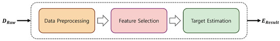
Figure 1.
Overall stream from raw data input to target estimation output.
3.1. Data Preprocessing
Data preprocessing is an important step in feature selection. In this step, the raw data are refined and converted into a suitable form for target estimation. In a multisensor system, each sensor may exhibit different characteristics and data formats, making appropriate preprocessing essential. Figure 2 illustrates the flow of sensor data preprocessing. The initial data collected by the sensor, denoted by , are trimmed and synchronized. Next, a missing value handling process is applied to address gaps in the data, followed by an outlier handling process. Finally, data scaling brings the data into a similar range, facilitating calculations between features. The final preprocessed data, , are then obtained.
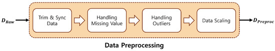
Figure 2.
Data preprocessing.
3.1.1. Synchronizing Data
In a multisensor system, synchronizing data from different sensors is crucial because each sensor may record data at different intervals or frequencies. Without proper synchronization, combining and analyzing the data can lead to inaccurate results or limited insights. Figure 3 shows (a) unsynchronized data and (b) synchronized data for the same dataset. As shown, synchronizing the data reveals the structure and characteristics more clearly. With multiple sensors, aligning the data across sensors is essential to ensure they share the same timeframe or event. Several strategies can be used to achieve synchronization:
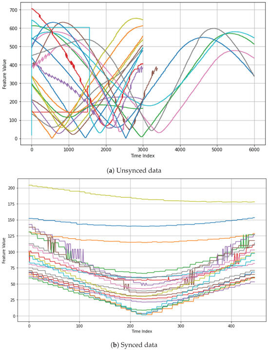
Figure 3.
Comparison of data before and after synchronization. The different colors in the graph represent each of the 20 experiments. (a) is the raw data, and (b) is the synchronized data, aligned to the point where the target is the closest.
- Time Alignment—Sensors may collect data at different rates, requiring resampling or interpolation techniques to align them to a common timeline. For example, data from faster sensors can be downsampled, or data from slower sensors can be interpolated to match the higher frequency.
- Identifying Synchronous Events—In certain cases, detecting events or triggers common to all sensors is helpful. Here, an “event” refers to a specific moment when all sensors simultaneously react during data collection. In this study, data from all sensors were aligned based on the closest target point to ensure synchronized timing across sensors. Events can therefore serve as synchronization points, with data aligned based on when each sensor detected the event.
Proper data synchronization ensures that inputs from multiple sensors are correctly aligned, enabling more accurate feature extraction and analysis.
3.1.2. Handling Missing Values
In the real world, missing data are frequently encountered due to sensor malfunctions, communication errors, or other technical problems. If not properly addressed, missing values can introduce bias during the feature selection process and reduce model performance. Several techniques are available for handling missing values [19,20].
- Listwise deletion—Removes all observations with missing values. While simple, this method can lead to significant data loss.
- Mean substitution—Replaces the missing values with the mean of variables. Although this method is also easy to use, this can reduce data variability, potentially distorting relationships between sensors, especially if the missing data are not random.
- Regression substitution—Predicts missing values by using other variables in a regression model, assuming a linear relationship. However, if this assumption is incorrect, it would lead to bias.
- Multiple imputation—Creates multiple datasets with different imputed values and combines the results, preserving variability and reducing bias.
Since the data in this study were not randomly generated, we used multiple imputation to handle missing data, replacing missing values with new values closely related to the nearest neighbors.
3.1.3. Handling Outliers
Outliers are extreme values that differ significantly from the rest of the data. In a multisensor system, outliers can result from sensor errors or environmental factors [21]. A multisensor setup makes identifying outliers more challenging due to differences in sensor characteristics and value ranges. Setting appropriate thresholds for identifying outliers is crucial, as mishandling them can negatively impact model training and lead to incorrect interpretations of results. Therefore, selecting outliers with a suitable method from various outlier detection techniques is essential.
Outlier Detection Methods:
- Z-score method—Identifies outliers by comparing data based on mean and standard deviation. It is most effective for data that follow a normal distribution.
- Interquartile range (IQR) method—Uses the first and third quartiles to detect outliers. It is robust and can handle skewed distributions, making it suitable for various data types.
- Density-based spatial clustering of applications with noise (DBSCAN)—As a clustering algorithm that identifies outliers based on data point density, it works well for complex distributions, but the effectiveness depends on careful parameter tuning.
Once the outliers have been identified, the next step is to determine how to handle these outliers. In this process, it is essential to select a method that best preserves the original structure of the input data.
Outlier Handling Methods:
- Removing Outliers—In cases where outliers are clearly due to errors or noise, they can simply be removed from the dataset. However, this can result in data loss, requiring caution, especially if the outliers represent important events.
- Imputation with Mean/Median—Outliers can be replaced with the mean or median of the data, especially when they are few in number. Median imputation is particularly useful for skewed data, as it is less sensitive to extreme values than the mean.
- Winsorizing—Involves capping the extreme values to a specific percentile range (e.g., the 5th and 95th percentiles) to reduce the influence of outliers without completely removing them from the dataset.
- K-nearest neighbors (KNN) regression—After detecting outliers (e.g., using the Z-score method), KNN regression can be applied to correct the outlier values, whereby outliers are replaced with predicted values based on the K-nearest data points, ensuring that the imputed values are consistent with the surrounding data.
- Transformation—Applying mathematical transformations (e.g., log or square root) can reduce the effect of outliers. This method is effective when outliers are due to skewed distributions.
In this study, the Z-score method was used to detect outliers. We incrementally adjusted the Z-score hyperparameter to identify a threshold that minimizes the number of detected outliers. The percentages of outliers at various Z-score thresholds are shown in Table 1. A higher Z-score threshold indicates that only points farther from the data center are considered outliers. Experimental results showed that setting the threshold to 7 or 8 effectively identified outliers while classifying minimal data as outliers.

Table 1.
Outlier percentages for different Z-score thresholds.
We then applied KNN regression to handle the detected outliers. The calculation for KNN regression is expressed as follows:
where x denotes the new data point; is the ith training data point; is the jth feature of the new data point; and is the jth feature of the ith training data point.
where is the predicted value for the new data point; K is the number of nearest neighbors; and is the target value of the ith nearest neighbor.
Figure 4 illustrates before and after handling outliers for the same data. (a) shows the dataset with outliers, which make it difficult to visualize the actual data, and (b) shows the dataset with outliers removed. Handling outliers allows for clearer visualization of the data distribution, which helps in further processing the task and data interpretation. Handling outliers enhances data clarity and data refinement for model training.
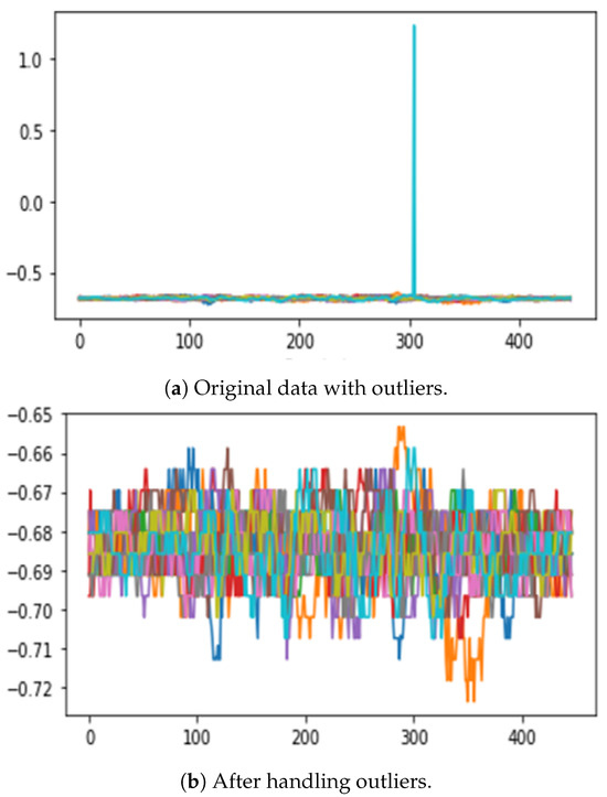
Figure 4.
Comparison of data before and after outlier handling. The different colors in the graph represent each of the 20 experiments. (a) shows the data with outliers and (b) shows the data after outlier removal, which allows for clearer visualization.
3.1.4. Scaling
After handling missing values and outliers, scaling is necessary. This step is essential because data collected from different sensors vary in units and ranges [22]. Scaling [23] is a technique that transforms data into a specific range, minimizing size differences between variables. It is applied independently to each feature, ensuring that no single feature’s scale dominates others during model training. Five different scaling techniques were used to determine the optimal scaler for the data.
- Standard scaling, also known as Z-score normalization, transforms the data to have a mean of 0 and a standard deviation of 1.where X is the original value; is the mean of the feature; and is the standard deviation. Standard scaling relies solely on mean and standard deviation, which does not constrain the data to a specific range. As a result, it is more susceptible to the influence of outliers.
- MinMax scaling, in contrast to standard scaling, rescales the data to a fixed range, typically between 0 and 1.where and represent the minimum and maximum values of the features, respectively. Since MinMax scaling relies on the minimum and maximum values of the data, it is highly sensitive to outliers, making outlier removal an essential preprocessing step.
- Robust scaling is designed to handle data with significant outliers by using the median and the interquartile range (IQR) instead of the mean and standard deviation. IQR is defined as the difference between the 25th and 75th percentiles.
- MaxAbs scaling scales each feature by dividing it by the maximum absolute value of that feature, ensuring that the range of the scaled data lies between −1 and 1.where is the maximum absolute value of the feature.
- Normalization [24] refers to adjusting the magnitude of each data point such that the data are represented as a vector of unit size. A common normalization method is L2 normalization, which scales each data point by the L2 norm (Euclidean norm) of the vector.where v is the original vector, and is the L2 norm. Normalization can also help reduce training times.
The main difference between scaling and normalization lies in their focus. Scaling adjusts the range and distribution of feature values, while normalization modifies the sizes of individual samples. Figure 5 shows the modified data after applying four different scaling and normalization techniques. By implementing the preprocessing steps of synchronizing data, addressing missing values, handling outliers, and applying appropriate scaling or normalization, robust and consistent datasets are obtained. These preprocessed data form the foundation for subsequent analysis and modeling steps, ensuring that the target is effectively learned and predicted from the sensor data.
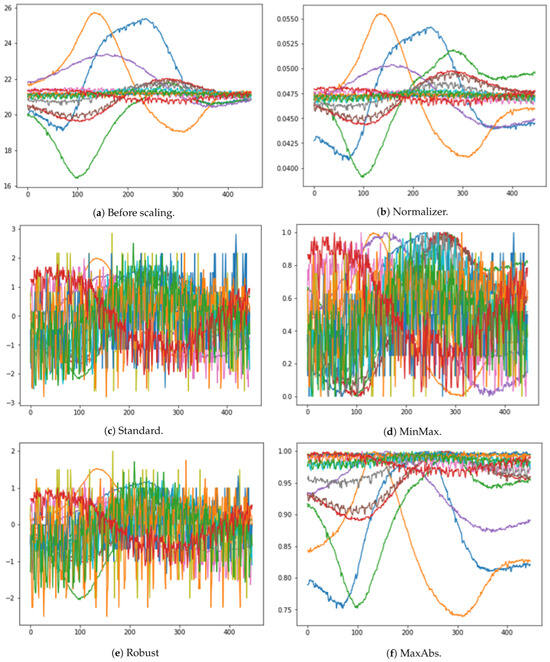
Figure 5.
Results for various scaling methods. The different colors in the graph represent each of the 20 experiments. (a) shows the visualization of the original data without any applied scaling. (b–f) display the visualizations for each of the different scaling methods.
3.2. Feature Selection
At this stage, the data are ready for model training. However, using all the sensor data may lead to extended training times, and it is uncertain whether all features are effective for target estimation.
Feature selection is a crucial step in the estimation process for several reasons. First, it improves model performance by eliminating irrelevant or redundant features, allowing the model to focus on the most important ones. This also helps prevent overfitting, enabling the model to generalize better to unseen data. Second, it enhances interpretability, making it easier to understand the relationships between input variables and model predictions. Third, it reduces computational complexity and training time by removing unnecessary features, which is particularly beneficial when dealing with large datasets. Finally, it addresses the problem of dimensionality and reduces noise in the dataset, contributing to more accurate predictions.
In this study, we simulate marine environmental conditions using sensor readings taken at distances ranging from 10 m to a maximum of 700 m. Due to the underwater setting and the long range of measurements, there is a high likelihood of unwanted noise, which can cause instability regardless of sensor performance. Conventional feature selection methods may carry over this environment-induced instability. To address this issue, we propose a hierarchical feature selection approach that first assesses the stability of each sensor, followed by selecting key sensors based on their relevance to the target variable. This hierarchical approach aims to achieve effective feature selection while minimizing instability challenges specific to the marine environment. Figure 6 illustrates the feature selection process used in this study.
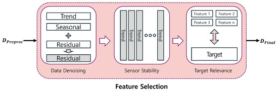
Figure 6.
Feature selection.
3.2.1. Denoising
The previous preprocessing step addressed outliers caused by input errors. However, noise inherent to long-range sensor measurements in marine environments, as well as potential physical noise from the sensors, has not yet been mitigated. Reducing such noise is essential to obtain a clearer representation of the data, which leads to more meaningful and interpretable results.
To address this, we applied Seasonal and Trend decomposition using Loess (STL) [25] to remove noise. Originally developed as a filtering procedure for decomposing seasonal time series data, STL divides the time series data into trend, seasonality, and residual components. The trend component represents the data’s long-term progression, the seasonal component captures repeated short-term patterns or cycles, and the residual component accounts for irregular or noise-like fluctuations not captured by the trend or seasonality. Since our data contain time series information, we applied STL decomposition for noise detection, setting thresholds to restrict the residual component. Recombining the restricted residual then produces denoised sensor data. In STL decomposition, the period hyperparameter determines the cycle length for the time series data. The choice of period should align with the specific patterns or trends within the data. In this study, since sensor data were collected in seconds, the period was set to 60. The basic form of STL decomposition is formulated as follows:
where T, S, and R represent the trend, seasonality, and residual, respectively; t is the time; and y represents the total original data.
Figure 7 illustrates how STL decomposition works. After residual data were obtained, we set three residual-restricting thresholds. We employ three different thresholds to limit the residuals from STL decomposition, referred to as Standard Range (SR), Quantile Range (QR), and a recomposition without residuals, which we designate as Trend Seasonality (TS) for simplicity. Based on the figure, we can confirm that the three thresholds are evenly distributed. If a stricter threshold (e.g., recomposition without residuals) yields improved results, it may indicate a substantial level of noise within the data. Conversely, if a more conservative threshold (e.g., Quantile Range) yields better outcomes, it is likely to suggest that even the noise in the collected data may carry meaningful information.
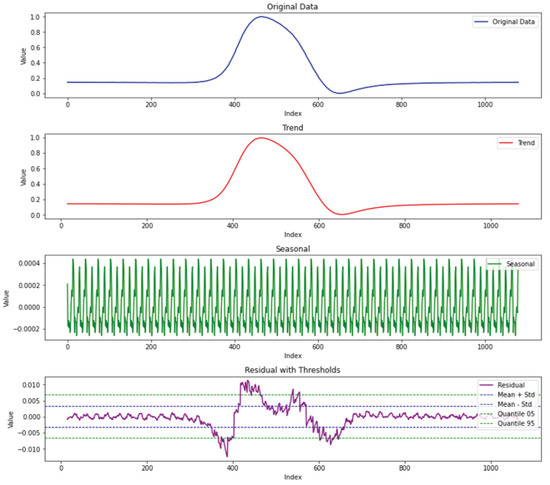
Figure 7.
STL decomposition example for magnetic field sensor data. The plots show the original, trend, seasonal, and residual components from the top, respectively. For residual-restricting thresholds in the last plot, the green dashed line is the quantile-based threshold which only restricts the top 5% and bottom 5% of residuals. The blue dashed line is the -based threshold.
Standard Range (SR) limits residuals within a range of the mean ± standard deviation. In this paper, is used. represents the mean of the residuals, and represents the standard deviation of the residuals. The adjusted residual is defined below:
The SR-denoised data , which recombine the trend and seasonality with the adjusted residual , are defined below:
Quantile Range (QR) limits residuals to exclude the upper and lower 5% of values, represented by and , respectively. Thus, the adjusted residual is defined below:
The QR-denoised data , which recombine the trend and seasonality with the adjusted residual , are then defined below:
Finally, Trend Seasonality (TS) data recombine only the trend and seasonality components, completely excluding the residual component. The TS denoised data are defined below:
Figure 8 presents regression results for all preprocessing combinations prior to feature selection. A total of 9 regressors including linear, ridge, lasso, decision tree, random forest, gradient boosting, KNN, and SVR are shown with different marker shapes. Colors indicate the scaling methods, with gray for MinMax, orange for standard, green for robust, purple for MaxAbs, and blue for Normalizer. To indicate STL denoising thresholds, filled markers represent SR, black-outlined markers represent QR, and empty markers represent TS. This figure plots the results of approximately 2700 experiments, applying these variations across around 20 different datasets.
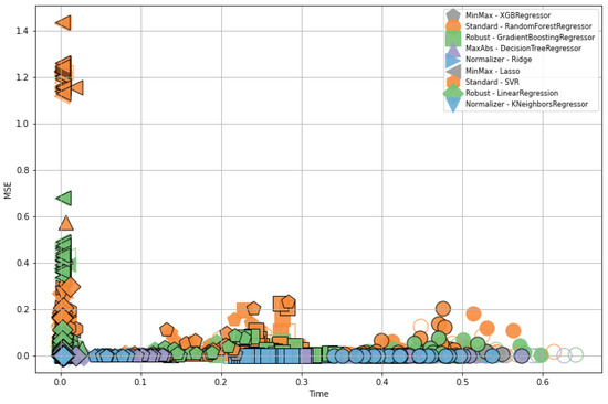
Figure 8.
Regression results for all preprocessing combinations before feature selection. Different marker shapes represent the 9 regressors, while color variations indicate the 5 scaling methods. Filled markers denote the SR denoising threshold, markers with black outlines represent QR, and empty markers indicate TS. Shapes indicate the models, with pentagons for XGB, circles for RandomForest, squares for GradientBoosting, triangles for DecisionTree, right-pointing triangles for Ridge, left-pointing triangles for Lasso, hexagons for SVR, diamonds for Linear, and inverted triangles for KNeighbors. Colors represent the scalers, where gray is MinMax, orange is Standard, green is Robust, purple is MaxAbs, and blue is Normalizer.
3.2.2. Sensor Stability
Ideally, performing feature selection should involve a deep understanding of the characteristics and operating principles of each sensor. However, in practice, feature selection is often necessary even when such expertise is lacking. As a result, many previously studied feature selection techniques [8,9,12,26,27,28,29] have been explored to identify ‘good’ features. However, evaluating all possible feature combinations is time-consuming and inefficient. To address this issue, this study adopts a hierarchical structure that divides the feature selection process into two stages. The first stage assesses the reliability of each sensor to discard features with insufficient reliability. This approach enhances the model’s stability by minimizing the risk of selecting sensors with low stability that may occasionally show good performance. To ensure sensor stability, we verify whether each sensor consistently provides stable data across all experiments. Calculating directly from raw sensor data can incorporate even minor noise; therefore, we use STL decomposition to extract only the trend component. This straightforward approach enables the identification of malfunctioning or unreliable sensors, even without prior knowledge of their performance.
In the previous STL denoising step, we used only the residual component to recompose the data with restrained noise. Now, we apply STL decomposition to the denoised data and again split them into trend, seasonality, and residual components. This time, the trend is utilized to determine the tendencies of the features.
The core of this methodology is the hypothesis that the consistency of sensor data is indicative of sensor reliability. Assessing consistency is particularly important for sensor data that may have hardware errors. Therefore, for each feature, data from all datasets are collected, and the correlation between these datasets is calculated to evaluate consistency. The mean correlation for each feature is then computed along with its standard deviation.
Let be the trend obtained from the STL decomposition of feature l in the i-th dataset, where represents the l-th feature among k features. The correlation of the trends for feature l across all datasets was calculated as follows:
In the following calculation, and are the data points from the respective datasets and is the mean of the trend in data and . Therefore, the correlation between two data points is calculated as follows:
The average of the computed correlations for feature l is calculated as follows:
The standard deviation of the correlations for a feature l is calculated as follows:
Figure 9 presents the results for sensor stability. The x-axis represents each feature. The mean correlation of each feature is shown as a blue bar plot, while the red line represents the standard deviation. Features with a high mean correlation and low standard deviation indicate greater consistency. Sensors identified as unreliable had features with a mean correlation that sharply decreased from the left, reflecting a sudden drop in consistency. Based on the point where the mean correlation bar sharply declined, features were selected for removal.
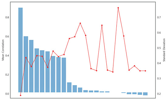
Figure 9.
Results of sensor stability. The blue bar chart represents the mean correlation, and the red line chart represents the standard deviation.
3.2.3. Target Relevance
After completing the sensor stability stage, the target relevance stage focuses on selecting features that are significantly related to target data estimation. This stage is based on the correlation between the target data and the features. In this study, a correlation technique was employed to identify sensors with a strong relationship to the target data, utilizing a basic filter method for feature selection to determine how each feature correlates with the target.
By examining these correlations, features that are highly related to the target variable are selected. This process is repeated across all datasets, with the most frequently appearing top features forming the final selected feature set. Through this hierarchical feature selection process, data dimensionality is reduced, and essential features are identified. Furthermore, this step-by-step approach yields a more accurate and efficient set of features, achieving high performance with reduced feature dimensions at minimal cost.
Figure 10 illustrates the regression results after applying all of the proposed methods. Compared to the previous Figure 8, only the Normalizer and TS threshold were applied, as these proved to be the optimal preprocessing methods for these data. As shown in the figure, both the mean square error (MSE) and processing time are significantly reduced. These results underscore the importance of data-specific preprocessing and demonstrate that the proposed hierarchical feature selection method achieves high performance.
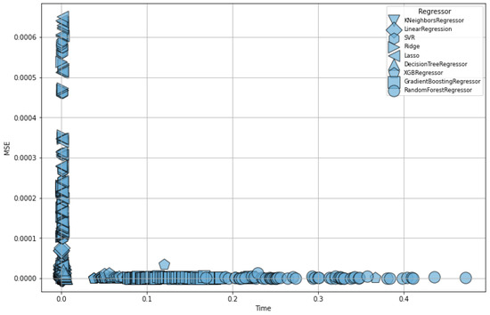
Figure 10.
Final regression results using the selected features, with Normalizer as the scaling method and TS as the denoising threshold.
4. Experiments and Results
4.1. Metrics
The evaluation indices in this study were based on MSE and . MSE, or mean square error, is primarily used for assessing the performance of regression models. It evaluates the magnitude of the prediction error by calculating the square mean of the differences between the actual and predicted values. Thus, a lower MSE indicates better model performance.
represents the performance of the model. is a value representing the degree of enhancement of the regression model relative to the average model, rather than dealing with the difference between the actual and predicted values, such as the MSE. If the value of is close to 0, it indicates that the regression model’s error divided by the average model’s error is close to 1, suggesting that the performance of the regression model is similar to that of the average model. Conversely, if is closer to 1, it signifies that the model is achieving better performance than the average model. The formulas for MSE and are as follows:
where is the actual value, is the predicted value, and n is the number of observations.
where r represents the Pearson correlation coefficient; n represents the number of data points; is the sum of the product of paired scores; and are the sums of the x and y scores, respectively; and and are the sums of the squares of the x and y scores, respectively.
4.2. Regression Models
For target estimation illustrated in Figure 11, we used a total of 9 regression models and long short-term memory (LSTM) [30] to evaluate the effectiveness of the data preprocessing and feature selection techniques. We aim to assess how well target estimation performs using only the features ultimately selected through these models. Additionally, we seek to verify whether the STL denoising and hierarchical feature selection methods proposed in this paper consistently demonstrate their effectiveness across various models. From the previously processed data, only the data corresponding to the finally selected sensors are used for training and target estimation. Each model had various strengths, weaknesses, and characteristics, which helped prove that the proposed techniques can assure generalization. A brief description of the 9 regression models and the LSTM is provided below:
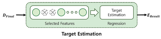
Figure 11.
Target estimation.
The most basic regression model, linear regression [31,32], is simple and easy to interpret but requires assumptions about linear relationships. Ridge regression [33] and LASSO regression [15], which apply L2 and L1 regularization, respectively, extend linear regression to prevent overfitting and facilitate variable selection. The decision tree regressor proposed by Breiman et al. [34] leverages an intuitive tree structure to achieve high performance. Building on this, the random forest regressor [34] ensembles multiple decision trees to improve prediction accuracy, reduce overfitting, and measure variable importance while also demonstrating robustness to noise.
Friedman’s gradient boosting regressor [35], based on a boosting algorithm that iteratively corrects errors in previous models, exhibits high adaptability to complex data. Similarly, XGBRegressor [36], which uses the extreme gradient boosting algorithm, provides superior prediction performance and a fast learning speed. The KNeighbors regressor [37], which is based on the K-nearest neighbor algorithm, enables a simple implementation by utilizing the proximity information in the data. Finally, support vector regressor (SVR) [38], proposed by Vapnik et al., is particularly advantageous for handling high-dimensional data and modeling nonlinear relationships. Hochreiter’s LSTM [39] is a type of recurrent neural network that is well suited for time series data and sequential learning tasks, allowing the capture of long-term dependencies and complex temporal patterns in the data.
4.3. Results
The approximately 3000 experimental results encompass typical marine environments, including scenarios where vessels approach from various directions and at different speeds, as well as measurements taken from sensors positioned in different locations. Through experimentation with multiple models, we demonstrated the effectiveness of the denoising and hierarchical feature selection methods proposed in this study. This underscores the importance of preprocessing techniques and feature selection methods that are well suited to the characteristics of the data being utilized.
Table 2 presents the results of the entire set of experiments, showing regression outcomes across five scaling methods and three threshold-based denoising techniques. These results are based on KNeighbors regression, the highest-performing model among the nine regressors evaluated. recursive feature elimination (RFE), a representative wrapper method for feature selection, was chosen as a baseline due to its stable performance and minimal hyperparameter requirements, needing only the final number of features to select, as shown in Figure 12. The proposed method, which takes a filter approach by considering the relationship with the target variable, was included to demonstrate that a simple and efficient filter method can surpass the performance of a wrapper method.
Table 2.
Quantitative results from KNeighbors regression demonstrate the effectiveness of the proposed denoising and feature selection methods, evaluated through MSE. For denoising, we individually applied three thresholds, where represents Standard Range, represents Quantile Range, and represents Trend Seasonality, a recomposition without residuals. Feature selection experiments were conducted in three ways. Feature selection experiments were conducted in three ways: first without feature selection, then using RFE as an existing feature selection method, and lastly with the hierarchical approach proposed in this study.
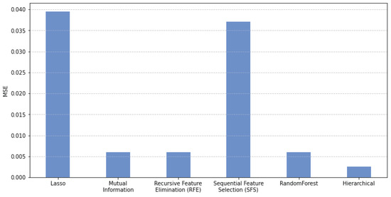
Figure 12.
Comparison of average MSE between different feature selection methods. Hierarchical method shows the lowest MSE among other methods.
In Table 2 and Figure 13, among the scaling methods, Normalizer demonstrated superior performance across all results. This may be attributed to the characteristics of the marine environment and sensors. Because Normalizer was applied on a row-wise basis, multisensors with a different range of values were effectively scaled. While other scaling methods adjusted the range within each sensor independently, ignoring inter-sensor relationships, Normalizer accounted for these relationships across sensors. Therefore, Normalizer appears to be well suited for the multisensor data in this experiment. This is particularly beneficial when the data contain variations in magnitude that reflect critical information about the system because Normalizer retains these relationships without distorting the inherent structure of the data.
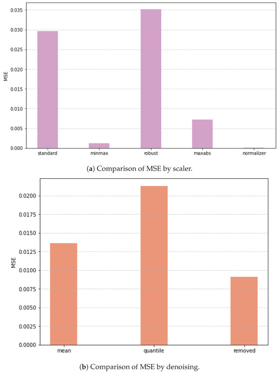
Figure 13.
Comparison of the average MSE across different scaler methods and denoising thresholds. (a) shows the graph for 5 scaler methods, showing that the Normalizer yields the lowest average MSE. (b) shows the graph for 3 denoising thresholds, with the TS threshold achieving the lowest average MSE.
The strong performance of the TS threshold, which most effectively reduces noise, suggests a significant amount of unnecessary noise in the sensor data. This implies that imposing strict noise constraints to simplify the sensor data yields better results. In this paper, this indicates that preserving only the major variations in sensor readings, rather than capturing finer fluctuations, leads to improved outcomes.
In Table 2, the performance of the proposed hierarchical feature selection method compared to traditional techniques is likely due to its ability to effectively exclude unreliable sensor data. By utilizing STL trend stability in the first step of the hierarchical feature selection process, problematic cases are filtered out, resulting in more reliable and stable outcomes. The selected features consistently identified the acoustic sensor as the most critical across all experimental results. Additionally, depth sensors and sensors acting on the z-axis followed in importance. This prioritization may be attributed to the acoustic sensor’s wide measurement range and sensitivity to minor variations, making it highly responsive to even subtle changes. The selected sensors closely mirror the target’s positional changes, indicating that these variations significantly contribute to target prediction.
Figure 14 visualizes actual sensor data to check the difference between sensors selected as important features and those that were not. Both the acoustic sensor and specific energy sensor share a characteristic where their values change more dynamically as they approach the center of the graph, where the target is the closest. However, the key difference between the two sensors lies in their consistency.
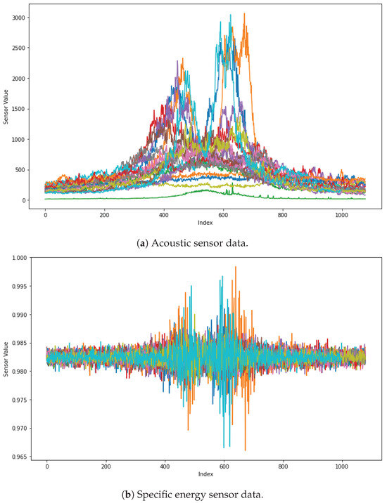
Figure 14.
Visualization of each sensor. The different colors in the graph represent each of the 20 experiments. (a) shows data from the acoustic sensor, which was frequently selected as a key sensor in the hierarchical feature selection process. In contrast, (b) shows data from the specific energy sensor, which was identified as less important. By examining these visualizations of the actual sensor data, we can assess the validity of the feature selection results.
For the acoustic sensor, nearly all data points display a consistent pattern—rising or falling together—which reflects a strong correlation with the target. In contrast, while the specific energy sensor exhibits a similar increase in activity near the center, it lacks the same level of consistency. Even at the same distance from the target, the specific energy sensor values vary significantly, suggesting that these values are influenced less by the proximity to the target and more by intrinsic fluctuations within the sensor itself. This indicates that the acoustic sensor provides a more reliable reflection of the target’s distance, while the specific energy sensor behaves more independently of the target, generating values that are less dependent on this context.
The experiment was conducted using an LSTM model to evaluate whether the proposed denoising and feature selection techniques are effective in deep learning models as well as in machine learning models. The LSTM model was trained for 100 epochs with a learning rate of 0.0005, using Adam optimizer with MSELoss. The input features were standardized, and the dataset was split into 80% for training and 20% for testing. Model evaluation was conducted using the R2 metric. Additionally, a dropout rate of 0.5 was applied during training to prevent overfitting.
The results of the experiment are presented qualitatively in Figure 15 and quantitatively in Table 3. The primary focus of the experiment was to assess the effect of feature selection using the STL denoising threshold, applied equally across the same dataset. The model performance was evaluated using the R2 value, where a higher R2 indicates better performance. As shown in Table 3, the average R2 value increases progressively when applying simple correlation-based feature selection without hierarchical methods and the proposed hierarchical feature selection technique on all the data. Although the results for existing feature selection appear to have been more favorable in some experiments, the high variability across multiple trials suggests that the proposed method delivers more consistently stable and reliable outcomes on average. This suggests that the proposed hierarchical feature selection method, which first assesses sensor stability in a two-stage process, provides robust results across diverse datasets.
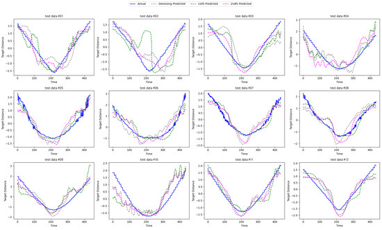
Figure 15.
Qualitative results for target estimation using LSTM. The graph represents the distance between sensors and the target. The x-axis represents time, whereas the y-axis represents target distance. The blue line shows the original target distance. Gray, green, and fuchsia dashed lines represent denoised, existing feature selection, and proposed hierarchical feature selection respectively.
Table 3.
Average R2 results for different feature selection methods using LSTM.
Figure 15 presents the results of target estimation using LSTM based on feature selection outcomes. The graph illustrates how well the model predicts the target as the vessel moves closer to and farther from the underwater sensors. Each test dataset represents an individual experimental dataset, showing target estimation results across a total of 12 experiments. The blue line represents the ground truth, while the dashed lines indicate experimental results: gray for denoising, green for feature selection using RFE, and fuchsia for the proposed hierarchical feature selection method. Notably, the fuchsia line closely follows the blue line, indicating that the proposed method achieves the most stable and accurate performance, even when using LSTM.
Table 4 provides a clear comparison of the effectiveness of the proposed denoising and feature selection methods. When the proposed feature selection method is applied, it demonstrates an approximate 99% reduction in MSE. These results emphasize the importance of appropriate preprocessing and feature selection techniques for sensor data analysis, demonstrating that these methods provide an effective solution for maritime target estimation, ensuring reliable and accurate predictions. By refining the data through systematic denoising and selecting the most relevant features, we showed that the proposed approach can significantly enhance model performance in real-world maritime environments, where sensor inconsistencies and noise often pose significant challenges. This reinforces the potential of these techniques as valuable tools for maritime navigation and target tracking.
Table 4.
MSE comparison of proposed method.
5. Discussion
We reviewed data denoising and feature selection techniques for maritime vessel estimation models using multisensor data. This step-by-step approach includes data verification, cleaning, outlier removal, scaling, STL denoising, and hierarchical feature selection, each tailored to the characteristics of sensor data. The experiment demonstrates how removing unnecessary data and selecting key features impacts results, highlighting the critical role of efficient data processing. These findings offer practical guidelines for processing sensor data during model construction across various domains.
Author Contributions
Conceptualization, S.C.; methodology, S.C.; software, S.C.; validation, S.C.; data curation, S.C.; writing—original draft preparation, S.C.; writing—review and editing, J.A.; visualization, S.C. All authors have read and agreed to the published version of the manuscript.
Funding
This work was supported by the National Research Foundation of Korea (NRF) grant funded by the Korea government (MSIT) (No. RS-2022-00165870) and the Gachon University research fund of 2023 (GCU-202400470001).
Institutional Review Board Statement
Not applicable.
Informed Consent Statement
Not applicable.
Data Availability Statement
The data presented in this study are available on request from the corresponding author due to privacy and ethical.
Conflicts of Interest
The authors declare no conflicts of interest.
Correction Statement
This article has been republished with a minor correction to the Funding statement. This change does not affect the scientific content of the article.
References
- Welch, H.; Clavelle, T.; White, T.D.; Cimino, M.A.; Van Osdel, J.; Hochberg, T.; Kroodsma, D.; Hazen, E.L. Hot spots of unseen fishing vessels. Sci. Adv. 2022, 8, eabq2109. [Google Scholar] [CrossRef] [PubMed]
- Paolo, F.S.; Kroodsma, D.; Raynor, J.; Hochberg, T.; Davis, P.; Cleary, J.; Marsaglia, L.; Orofino, S.; Thomas, C.; Halpin, P. Satellite mapping reveals extensive industrial activity at sea. Nature 2024, 625, 85–91. [Google Scholar] [CrossRef] [PubMed]
- Orofino, S.; McDonald, G.; Mayorga, J.; Costello, C.; Bradley, D. Opportunities and challenges for improving fisheries management through greater transparency in vessel tracking. ICES J. Mar. Sci. 2023, 80, 675–689. [Google Scholar] [CrossRef]
- Watson, J.T.; Ames, R.; Holycross, B.; Suter, J.; Somers, K.; Kohler, C.; Corrigan, B. Fishery catch records support machine learning-based prediction of illegal fishing off US West Coast. PeerJ 2023, 11, e16215. [Google Scholar] [CrossRef]
- Wu, P.; Zhang, H.; Shi, Y.; Lu, J.; Li, S.; Huang, W.; Tang, N.; Wang, S. Real-time estimation of underwater sound speed profiles with a data fusion convolutional neural network model. Appl. Ocean Res. 2024, 150, 104088. [Google Scholar] [CrossRef]
- Yang, M.; Sha, Z.; Zhang, F. A Multi-Modal Approach Based on Large Vision Model for Close-Range Underwater Target Localization. arXiv 2024, arXiv:2401.04595. [Google Scholar]
- Ge, X.; Zhou, H.; Zhao, J.; Li, X.; Liu, X.; Li, J.; Luo, C. Robust Positioning Estimation for Underwater Acoustics Targets with Use of Multi-Particle Swarm Optimization. J. Mar. Sci. Eng. 2024, 12, 185. [Google Scholar] [CrossRef]
- Chandrashekar, G.; Sahin, F. A survey on feature selection methods. Comput. Electr. Eng. 2014, 40, 16–28. [Google Scholar] [CrossRef]
- Li, J.; Cheng, K.; Wang, S.; Morstatter, F.; Trevino, R.P.; Tang, J.; Liu, H. Feature selection: A data perspective. ACM Comput. Surv. (CSUR) 2017, 50, 1–45. [Google Scholar] [CrossRef]
- Bolón-Canedo, V.; Sánchez-Maroño, N.; Alonso-Betanzos, A. A review of feature selection methods on synthetic data. Knowl. Inf. Syst. 2013, 34, 483–519. [Google Scholar] [CrossRef]
- Hall, M.A. Correlation-Based Feature Selection for Machine Learning. Ph.D Thesis, The University of Waikato, Hamilton, New Zealand, 1999. [Google Scholar]
- Peng, H.; Long, F.; Ding, C. Feature selection based on mutual information criteria of max-dependency, max-relevance, and min-redundancy. IEEE Trans. Pattern Anal. Mach. Intell. 2005, 27, 1226–1238. [Google Scholar] [CrossRef] [PubMed]
- Guyon, I.; Weston, J.; Barnhill, S.; Vapnik, V. Gene selection for cancer classification using support vector machines. Mach. Learn. 2002, 46, 389–422. [Google Scholar] [CrossRef]
- Bouaguel, W. A new approach for wrapper feature selection using genetic algorithm for big data. In Intelligent and Evolutionary Systems: Proceedings of the 19th Asia Pacific Symposium, IES 2015, Bangkok, Thailand, 22–25 November 2015; Proceedings; Springer International Publishing: Cham, Switzerland, 2016; pp. 161–171. [Google Scholar]
- Tibshirani, R. Regression shrinkage and selection via the lasso. J. R. Stat. Soc. Ser. B Stat. Methodol. 1996, 58, 267–288. [Google Scholar] [CrossRef]
- Zou, H.; Hastie, T. Regularization and variable selection via the elastic net. J. R. Stat. Soc. Ser. B Stat. Methodol. 2005, 67, 301–320. [Google Scholar] [CrossRef]
- Khaleghi, B.; Khamis, A.; Karray, F.O.; Razavi, S.N. Multisensor data fusion: A review of the state-of-the-art. Inf. Fusion 2013, 14, 28–44. [Google Scholar] [CrossRef]
- Fernández-Delgado, M.; Sirsat, M.S.; Cernadas, E.; Alawadi, S.; Barro, S.; Febrero-Bande, M. An extensive experimental survey of regression methods. Neural Netw. 2019, 111, 11–34. [Google Scholar] [CrossRef]
- Bilal, M.; Ali, G.; Iqbal, M.W.; Anwar, M.; Malik, M.S.A.; Kadir, R.A. Auto-prep: Efficient and automated data preprocessing pipeline. IEEE Access 2022, 10, 107764–107784. [Google Scholar] [CrossRef]
- Tharwat, A.; Schenck, W. Active Learning for Handling Missing Data. IEEE Trans. Neural Netw. Learn. Syst. 2024. [Google Scholar] [CrossRef]
- Rousseeuw, P.J.; Hubert, M. Robust statistics for outlier detection. Wiley Interdiscip. Rev. Data Min. Knowl. Discov. 2011, 1, 73–79. [Google Scholar] [CrossRef]
- Ahsan, M.M.; Mahmud, M.P.; Saha, P.K.; Gupta, K.D.; Siddique, Z. Effect of data scaling methods on machine learning algorithms and model performance. Technologies 2021, 9, 52. [Google Scholar] [CrossRef]
- Torgerson, W.S. Theory and Methods of Scaling; Wiley: Hoboken, NJ, USA, 1958. [Google Scholar]
- Patro, S.G.; Sahu, K.K. Normalization: A preprocessing stage. arXiv 2015, arXiv:1503.06462. [Google Scholar] [CrossRef]
- Cleveland, R.B.; Cleveland, W.S.; McRae, J.E.; Terpenning, I. STL: A seasonal-trend decomposition. J. Off. Stat. 1990, 6, 3–73. [Google Scholar]
- Venkatesh, B.; Anuradha, J. A review of feature selection and its methods. Cybern. Inf. Technol. 2019, 19, 3–26. [Google Scholar] [CrossRef]
- Khalid, S.; Khalil, T.; Nasreen, S. A survey of feature selection and feature extraction techniques in machine learning. In Proceedings of the 2014 Science and Information Conference, London, UK, 27–29 August 2014; pp. 372–378. [Google Scholar]
- Gerretzen, J.; Szymanska, E.; Jansen, J.J.; Bart, J.; van Manen, H.J.; van den Heuvel, E.R.; Buydens, L.M. Simple and effective way for data preprocessing selection based on design of experiments. Anal. Chem. 2015, 87, 12096–12103. [Google Scholar] [CrossRef] [PubMed]
- Karagiannopoulos, M.; Anyfantis, D.; Kotsiantis, S.B.; Pintelas, P.E. Feature selection for regression problems. In Proceedings of the 8th Hellenic European Research on Computer Mathematics & Its Applications, Athens, Greece, 20–22 September 2007. [Google Scholar]
- Wu, X.; Kumar, V.; Ross Quinlan, J.; Ghosh, J.; Yang, Q.; Motoda, H.; McLachlan, G.J.; Ng, A.; Liu, B.; Yu, P.S.; et al. Top 10 algorithms in data mining. Knowl. Inf. Syst. 2008, 14, 1–37. [Google Scholar] [CrossRef]
- Guo, Y.; Wang, W.; Wang, X. A robust linear regression feature selection method for data sets with unknown noise. IEEE Trans. Knowl. Data Eng. 2023, 35, 31–44. [Google Scholar] [CrossRef]
- Hassani, H.; Mahmoudvand, R.; Yarmohammadi, M. Filtering and denoising in linear regression analysis. Fluct. Noise Lett. 2010, 9, 367–383. [Google Scholar] [CrossRef]
- Hoerl, A.E.; Kennard, R.W. Ridge regression: Biased estimation for nonorthogonal problems. Technometrics 1970, 12, 55–67. [Google Scholar] [CrossRef]
- Breiman, L. Random forests. Mach. Learn. 2001, 45, 5–32. [Google Scholar] [CrossRef]
- Friedman, J.H. Greedy function approximation: A gradient boosting machine. Ann. Stat. 2001, 29, 1189–1232. [Google Scholar] [CrossRef]
- Chen, T.; Guestrin, C. XGBoost: A scalable tree boosting system. In Proceedings of the 22nd ACM SIGKDD International Conference on Knowledge Discovery and Data Mining, San Francisco, CA, USA, 13–17 August 2016; ACM: New York, NY, USA, 2016; pp. 785–794. [Google Scholar]
- Cover, T.M.; Hart, P.E. Nearest neighbor pattern classification. IEEE Trans. Inf. Theory 1967, 13, 21–27. [Google Scholar] [CrossRef]
- Drucker, H.; Burges, C.J.; Kaufman, L.; Smola, A.; Vapnik, V. Support vector regression machines. In Proceedings of the 9th International Conference on Neural Information Processing Systems (NIPS), Denver, CO, USA, 2–5 December 1996; MIT Press: Cambridge, MA, USA, 1996; pp. 155–161. [Google Scholar]
- Hochreiter, S. Long Short-term Memory. Neural Comput. 1997, 9, 1735–1780. [Google Scholar] [CrossRef]
Disclaimer/Publisher’s Note: The statements, opinions and data contained in all publications are solely those of the individual author(s) and contributor(s) and not of MDPI and/or the editor(s). MDPI and/or the editor(s) disclaim responsibility for any injury to people or property resulting from any ideas, methods, instructions or products referred to in the content. |
© 2024 by the authors. Licensee MDPI, Basel, Switzerland. This article is an open access article distributed under the terms and conditions of the Creative Commons Attribution (CC BY) license (https://creativecommons.org/licenses/by/4.0/).