Abstract
For a forward-bending biped robot with 10 degrees of freedom on its legs, a new control framework of MPC-DCM based on force and moment is proposed in this paper. Specifically, the Diverging Component of Motion (DCM) is a stability criterion for biped robots based on linear inverted pendulum, and Model Predictive Control (MPC) is an optimization solution strategy using rolling optimization. In this paper, DCM theory is applied to the state transition matrix of the system, combined with simplified rigid body dynamics, the mathematical description of the biped robot system is established, the classical MPC method is used to optimize the control input, and DCM constraints are added to the constraints of MPC, making the real-time DCM approximate to a straight line in the walking single gait. At the same time, the linear angle and friction cone constraints are considered to enhance the stability of the robot during walking. In this paper, MATLAB/Simulink is used to simulate the robot. Under the control of this algorithm, the robot can reach a walking speed of 0.75 m/s and has a certain anti-disturbance ability and ground adaptability. In this paper, the Model-H16 robot is used to deploy the physical algorithm, and the linear walking and obstacle walking of the physical robot are realized.
1. Introduction
It is well known that the biped robot is a relatively complex model in the field of control. In the process of walking, it is necessary to maintain the static or dynamic balance of the system on the basis of considering the synchronous operation of multiple motors. Among them, static walking requires that the projection of the center of mass is always inside the support polygon to ensure balance at any time, but high balance also limits its walking speed [1]. The walking speed of Honda’s ASIMO robot [2] can only reach 0.44 m/s, representing a high level of static walking research. Dynamic walking relaxes the restriction of the projection position of the center of mass and uses the horizontal component of the ground reaction force to push the robot to move in the horizontal plane, which is similar to the running behavior of humans. The typical dynamic walking model is the Linear Inverted Pendulum Model (LIPM).
Due to the high-order, multi-variable, and strongly coupled characteristics of the biped robot model, it is extremely difficult to establish the model and the direct control is more complex. Dominguez [3] proposed the Linear Inverted Pendulum Model (LIPM) to establish the simplified dynamics of the biped robot. Many scholars have used LIPM in the field of biped robots for research. Caron [4] considered the change in the height of the centroid on the basis of the traditional LIPM, analyzed the feasible region of the centroid in the case of terrain changes, and carried out the planning of the centroid trajectory. Guan [5] proposed a virtual mass ellipsoid inverted pendulum model with varying angular momentum and height of the center of mass, and Li [6] applied LIPM to 3D complex environments to realize complex actions such as stair climbing.
DCM is also developed on the basis of LIPM. Pratt [7] first considered the problem of when and where the robot should land and proposed the concept of Capture Point (CP), which means that the robot can stop completely at the CP. Subsequent scholars have also made complementary developments to Pratt’s theory. Hof proposed the concept of extrapolated centroid similar to the CP point of Pratt’s theory and used the extrapolated centroid to plan the walking and stability control of biped robots. Kajita [8] proposed the concept of orbital energy in his research and pointed out that the point with zero orbital energy is the point where the linear inverted pendulum system can completely stop, and the projection of the point with zero orbital energy on the ground is the Capture Point (CP) proposed by Pratt [7]. Takenaka [9] and Englsberger [10] found in their study of the linear inverted pendulum that LIPM could be decoupled in the complex frequency domain to obtain the essentially divergent part—Motion Divergent Component (DCM). After calculation, DCM was consistent with Pratt’s capture point theory.
In the research direction of DCM, Englsberger [11] proposed two real-time anti-disturbance DCM strategies: CPT (Capture Point Tracking) and CPS (Capture Point End-of-step). Young-Dae Hong began to use a DCM walking planning strategy based on an optimization method and used a particle swarm optimization algorithm to optimize the selection of capture points and centroid trajectories [12]. Han [13] proposes a novel DCM model prediction method to predict multiple footstep positions during a fixed walking cycle, enabling fast and relevant footstep selection for biped robots and facilitating fast recovery of robot velocity. Morisawa [14] established a typical 12-DOF control scheme based on DCM theory and ZMP programming and realized the real-time tracking of the desired ZMP with limiting correction. Zhang Zhao [15] introduced the rolling optimization method of MPC to complete the real-time trajectory tracking of DCM, taking into account the influence of the angular momentum of the center of mass. Hopkins [16] and Griffin [17] used the time-varying DCM strategy to study the height variation of the center of mass during the walking process of a biped robot. However, they are all tested on 12 DOF fully controlled robots, and there is still a gap in the practical application of DCM theory for 10 DOF robots with more ground adaptability but less stability.
In this paper, the DCM of 10 DOF robots is studied. Due to the underactuated nature of the 10 DOF robots themselves, the force–torque control algorithm is adopted in this paper. Based on the linear inverted pendulum, the dynamic equilibrium equation is established by the reaction force of the foot end and the center of mass, and the mathematical description of the complete 10 DOF biped robot system is established by combining DCM theory. The rolling optimization method of MPC is used to track the target trajectory, and the optimal control input within the constraints is determined and applied to the robot entity.
In this paper, based on DCM theory and the MPC algorithm, we study and verify the control effect of the force–torque control algorithm on a 10-DOF biped robot. The main contributions of this paper are as follows:
- A new 10 DOF robot control framework is established by combining DCM theory and MPC algorithm.
- The constraint of DCM is added to the constraint conditions of MPC to enhance the stability of the system.
- A physical simulation model is established based on the Model-H16 robot.
- The feasibility and anti-interference ability of the algorithm are verified on the Model-H16 robot.
2. Model of Biped Robot
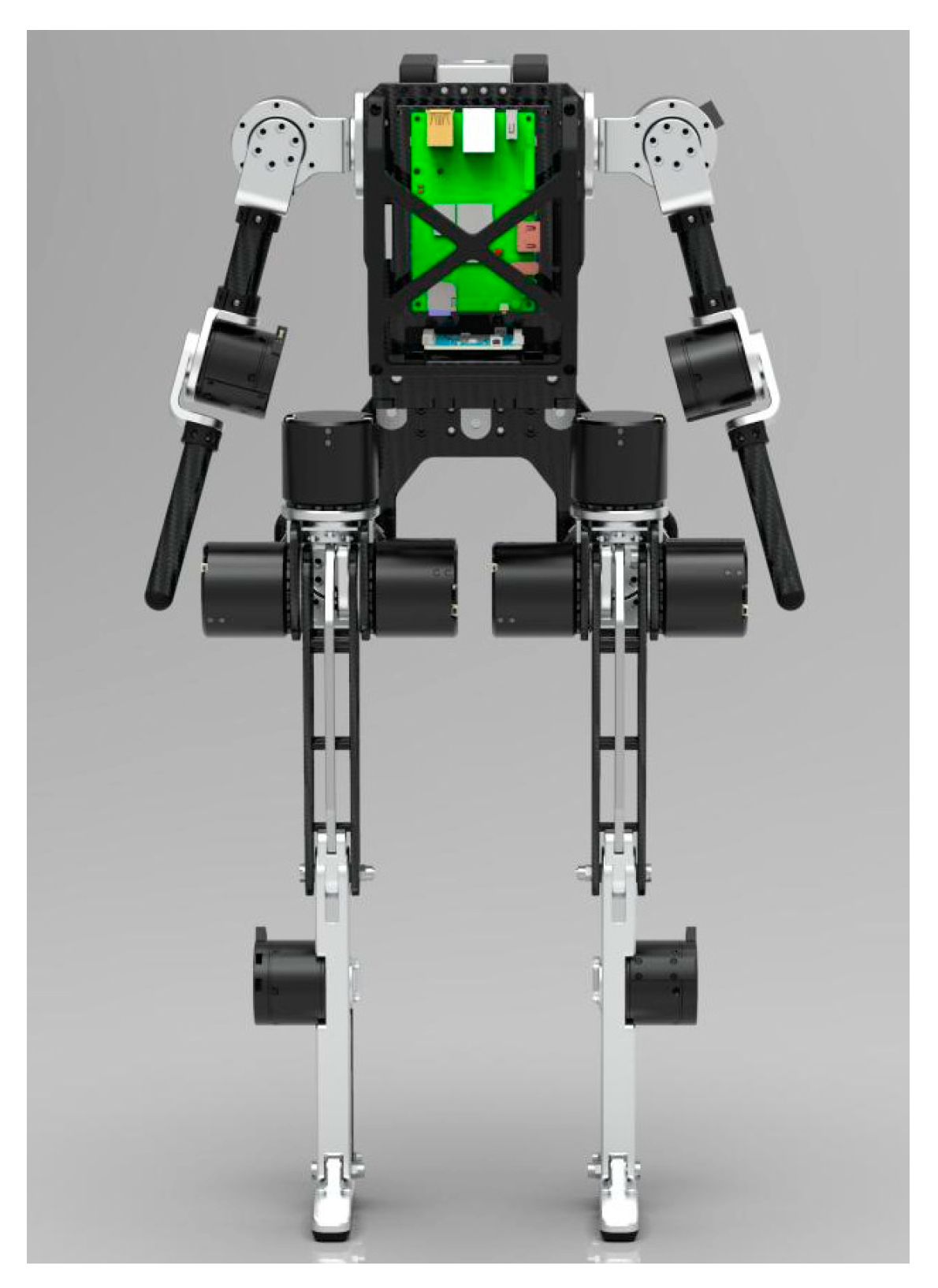
This section will introduce the biped robot simulation model and physical model information used in this paper. The simulation model and the physical model use the product Model-H16 robot produced by Gaoqing Electromechanical. Figure 1a shows the complete structure of the robot, and Figure 1b shows the motor, rotation axis, link, and other information about the robot leg. A photograph of the physical robot is presented in Figure 2.
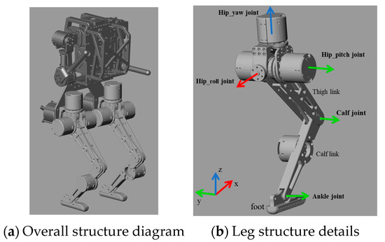
Figure 1.
Structure diagram of the Model-H16 robot.
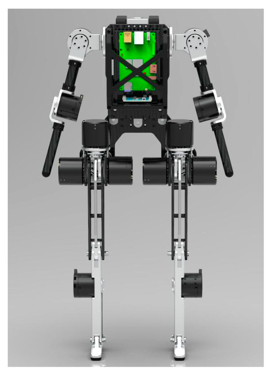
Figure 2.
Model-H16 robot physical photo.
The robot used in this paper is a bipedal robot with 10 degrees of freedom, and there are mainly two kinds of motors used. One kind of small motor, model HTM4538, is used in the ankle joint alone, and HTM5046 motors are used in the other four motors of the legs. The simple parameter ranges of the motors are shown in Table 1. Since this paper only considers the biped robot walking problem, the upper body structure of the Model-H16 robot is not involved.

Table 1.
Motor parameters of the Model-H16 robot.
The control structure of the system used in this paper is shown in Figure 3.
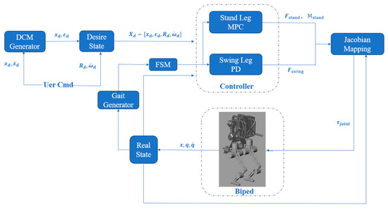
Figure 3.
Overall structure of the control system.
3. Dynamic Model Based on DCM
For a control system, in order to describe the system in a coded way and carry out corresponding control, it is necessary to establish a mathematical model of the system. Since the biped robot system is a complex system, considering the dynamics of all links makes the analysis extremely difficult. The common way is to simplify the complex biped robot. Since the mass of biped robot is mostly concentrated in the position of the center of mass battery, for the convenience of analysis, this paper simplifies it to LIPM without considering the mass of legs. At the same time, in order to improve the control effect of the system, DCM is introduced as the state variable, and the state transition matrix of the whole system is established.
3.1. Review of LIPM
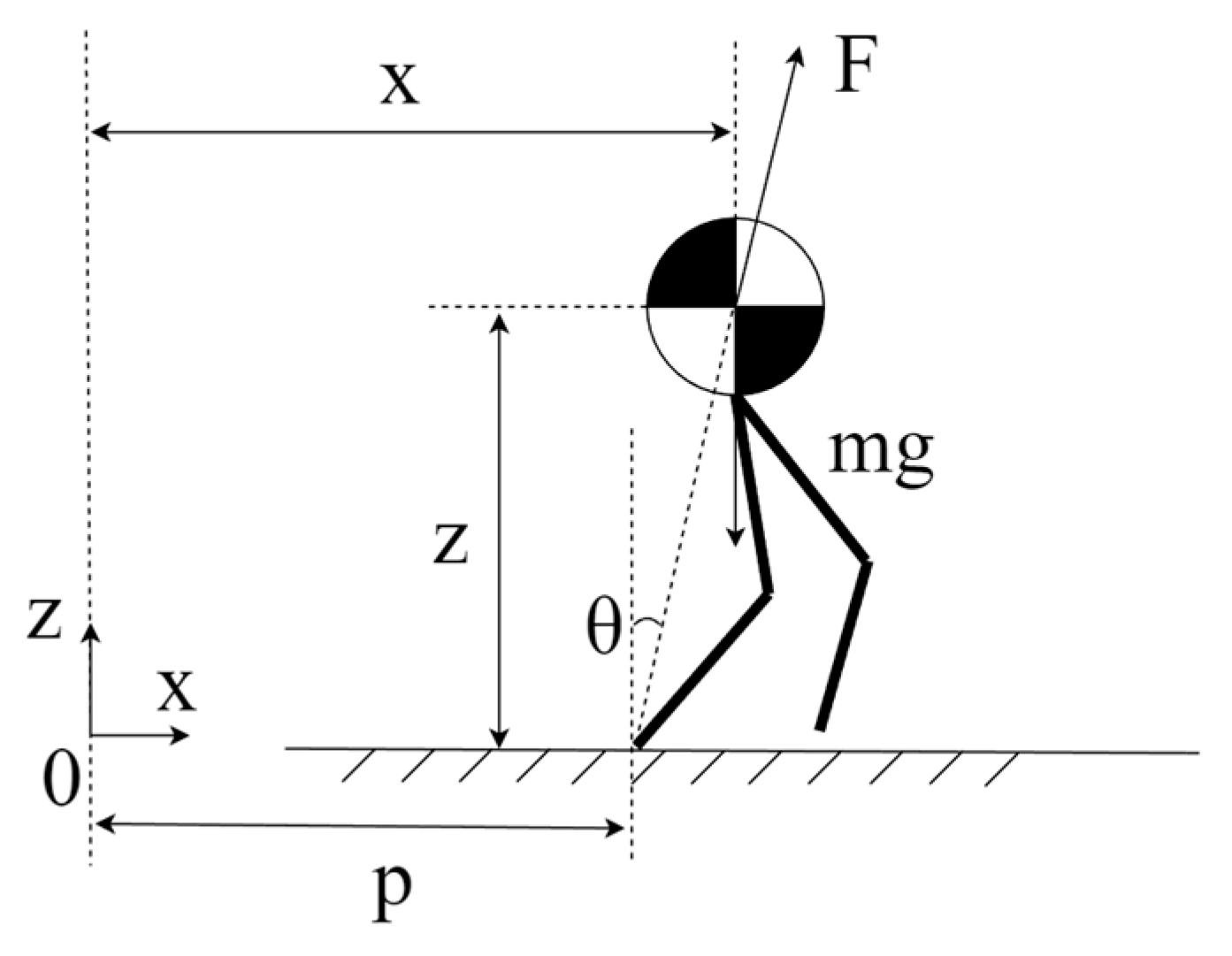
The Linear Inverted Pendulum Model regards the biped robot as a simple structure with a center of mass and a lightweight link, ignores many variables such as leg configuration, leg mass, ankle joint torque, and simplifies the biped robot, a multi-variable, strong-coupling and high-order system, into the simplified model shown in Figure 4 (only the schematic diagram in the x-z two-dimensional coordinates is shown, and the same is true in the y-z direction). A force analysis is performed on the center of mass of the robot and Equation (1) is derived as follows:
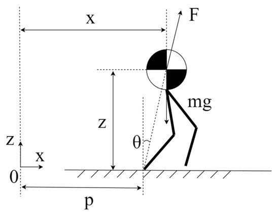
Figure 4.
Linear Inverted Pendulum Model image.
According to the force equation of the simplified model (1), the dynamic equation of the LIPM is obtained as expressed in Equation (2):
where .
3.2. Review of DCM
Equation (1) shows the relationship of ZMP–COM [18]. Pratt puts forward the concept of complete static at the Capture Point, and in the control theory treatment of Equation (2), Takenaka maps the relationship of ZMP–COM to the complex frequency domain, obtaining the divergence component in its process, which is consistent with the Capture Point concept mentioned above. In terms of formulas, this is expressed as Equation (2), where ε is the motion diverging component (or Capture Point, which is referred to as the Motion Diverging Component in this paper).
The first row in Equation (3) describes the relationship between DCM and the centroid, and the second row describes the relationship between DCM and the foothold ZMP. By eliminating the ZMP variable in Equation (2), the relationship between ε and the centroid state is obtained as Equation (4).
3.3. Dynamics
The traditional LIPM does not consider the influence of the foot end on the robot body, nor does it consider the torque of the foot end. In the actual robot system, because the foot end is rarely a point foot, there must be a certain foot moment. In order to achieve a better control effect and better ground adaptability, this paper will establish LIPM considering foot moment based on DCM. Inspired by the work of Li [19], the state variables of the system are selected as [centroid Euler angle, centroid position, centroid angular velocity, and motion divergence component].
The center of mass of the biped robot is basically kept upright during walking or other actions (other special cases are not considered), that is, roll and pitch are not considered in the Euler angle of the center of mass, only yaw angle is considered, and its angular velocity is obtained by the following Equations (5) and (6).
The linear velocity of the center of mass can be obtained according to the first row of Equation (2).
For the calculation of angular acceleration of the center of mass, considering LIPM, a single rigid body model, the mass is only concentrated in the center of mass, so the overall inertia matrix is the center of mass inertia matrix . Considering yaw offset of the center of mass as mentioned above, the new moment of inertia can be obtained through Equation (8).
Equation (9) for calculating angular acceleration can be obtained from Formula for calculating torque of rigid body kinematics.
In Equation (9), and represent the foot end forces of the left and right legs, respectively, and and represent the moments of the left and right legs, the derivative of the motion diverging component can be obtained by taking the derivative of Equation (3), as shown in Equation (10).
Combined with the force analysis of the center of mass, , where is the gravitational acceleration, and and are the ground reaction force of the right foot and the left foot, respectively. Finally, the derivative of DCM is obtained through Equation (11).
The dynamic model of the whole system obtained from all the above analysis is shown in Equation (12).
where ,
A =
B =
L =
=
3.4. Extended State
To unify the variables and facilitate subsequent processing, we add the gravity acceleration metric to the state quantity, and the state quantity is expanded to . The system matrix and input matrix of the extended state transition matrix are Equations (13) and (14).
The state transition matrix at this time is shown in Equation (15), Equation (15) is discretized to obtain Equation (16).
4. Controller of Support Leg
The dynamic model based on DCM is established in Section 3, and the control of the support leg will be considered in this part. Figure 3 shows the overall control block diagram of the system, which will be analyzed in detail by modules in this part.
4.1. MPC Controller
MPC (Model Predictive Control) is an optimization calculation method commonly used in the control field [20,21]. MPC is used in multiple-input multiple-output (MIMO) systems to calculate the control parameters when the loss function is lowest according to the system model, target state. and control input, which are particularly important in the foot robot. In this part, the typical MPC method is used to calculate the optimal foot state with the system model established in Section 3 and the target state entered by the user. The structure diagram of the controller is shown in Figure 5, where the inputs are the desired state and the actual state, and the output is the control input u of the state transition matrix.
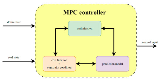
Figure 5.
The structure of the MPC controller.
Equation (17) is the loss function of the system. In this paper, the deviation of the state variable is selected as the process loss, the input is taken as the input loss, and , are the weight matrices of these two quantities, respectively. Equation (18) is the state transition matrix of the system, which is obtained in Equation (12). Equations (19) and (20) are the inequality and equality constraints of MPC. In this paper, both the state quantity and the input are constrained, and are the constraint aggregation matrices of the inequality and equality constraints, respectively.
4.2. Constraint Condition
4.2.1. Inequality Constraints
Friction Cone Constraint: In the stable walking process of the biped robot, in order to ensure the robustness of the robot’s walking, the position of the foot end should not change; that is, the plantar should not slip due to the action of the torque. This requirement requires that the component force of the ground reaction force in the x-y plane satisfies the friction cone constraint [22]. Equations (21) and (22) show the friction cone constraint in the x and y directions. Where is the static friction coefficient, , representing the left and right legs.
Motor Torque Constraints: All actions of the biped robot are affected by the torque of the left and right 10 motors, but the maximum torque of the motors is limited by the hardware of the motors. The robot adopted in this paper uses two types of motors (whose parameters are mentioned in Table 1, and the control torque imposed by the two types of motors should also be limited. According to the size, the biped robot is divided into two types: Equations (23) and (24).
Normal Force Constraint: Since the control target of this paper is the foot force and moment, the ground reaction force is particularly important. Besides the friction cone constraint, the ground reaction force also needs to control the normal force to ensure that the normal force is within a limited range and constantly upward. The formula can be summarized as Equation (25).
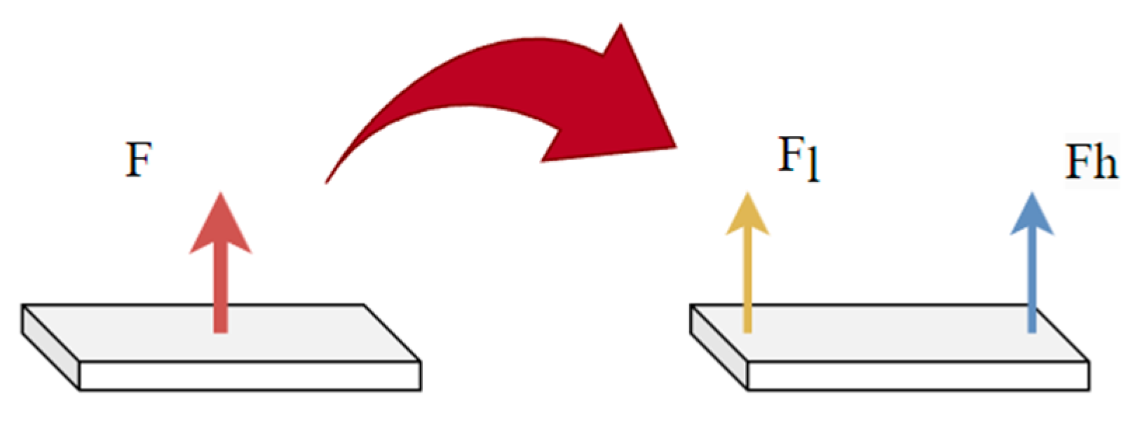
Line-Foot Contact: In order to consider the Line-Foot Contact constraint proposed by Caron [23], it is also necessary to constrain the contact lines of both feet. Due to the existence of the ankle pitch angle of the robot, it may make the feet point to the ground or the heel point to the ground. Therefore, based on Caron’s research, this algorithm constrains the ankle pitch angle, and the constraint method is as follows.
The plantar reaction force F is divided into yellow and blue parts in Figure 6, which act on the heel and the tip of the foot, respectively (since there is only pitch, the component force in the y direction is not considered). These two forces are and , and and , respectively; they are separated in the x and y directions, respectively.

Figure 6.
Foot ground force and its component force.
Equations (26) and (27) describe the splitting process in detail. The force at the heel and the tip of the foot is divided into two forces in the y direction and the z direction (the x direction does not exist), and then the relationship between the torque at the single point of action and the torque at the two positions during the ankle joint action is further considered. The torque splitting results are given by Equations (28) and (29).
Here, is the distance from the ankle to the heel, is the distance from the ankle to the tip of the foot, and are the torques at the action points of the ground reaction force, and and are the ground reaction forces at the action points of heel and toe.
Equations (26)–(29) are solved simultaneously to obtain the force in y and z directions at the heel and tip of the foot, as shown in Equation (30).
Equation (30) shows the y-direction component force of the heel of the tip of the foot, and these two components need to comply with the friction cone constraint, that is, . Combined with the above equation, the constraint conditions of the feet are completed.
DCM Line Constraint: In the MPC control framework proposed by Li [19], the DCM trajectory still has a curved part, which causes the corresponding centroid trajectory to exhibit a certain degree of abrupt change [9,24], thereby, the stability is still challenged to some extent. In this paper, the DCM is constrained in each single gait, so that the real-time DCM in the running process is straight to ensure the stability of the centroid trajectory in the x-y plane. The calculation constraint formula is given in Equation (31).
4.2.2. Equality Constraint
Since the biped robot model with 10 degrees of freedom is adopted in this paper, there is no ankle joint roll degree of freedom, and the ankle joint roll torque is not considered in the control objective, so the roll torque should always be 0 in the equality constraint, that is, Equation (32). The goal of this is to prevent the existence of roll torque, which makes the foot entity rotate. In single leg support, the support polygon is a straight line, which increases the risk of system instability.
4.3. QP Problem Solution
According to Equation (18), the state of the next sampling time can be calculated by using the state transition matrix of the system and the control input, and so on, the state of the K control input at the N sampling time can be calculated according to the time series. In this paper, K = 10 is selected as the control period of MPC, and all the prediction results within N = 10 periods are calculated. The state set is expressed by Equation (33).
where is the system state including the next 10 cycles, is the initial state, and is the optimal control input for a total of 10 cycles including the initial state. The objective function used in the MPC design is written in the following form:
where
Equation (34) is the simplified loss function, which is the QP quadratic standard form. Equations (35) and (36) are the aggregation of all inequality constraint constraints and equality constraints of the control cycle, respectively. In Equations (37) and (38), M represents the weight of state quantity change in the prediction period, and K is the change rate of MPC control input in the prediction period. Since the QP problem processes all state quantities and control inputs in the prediction period, M and K are the aggregation of state weight Q and control input weight R in Equation (17). Equations (39) and (40) represent this process.
where N is the number of prediction periods.
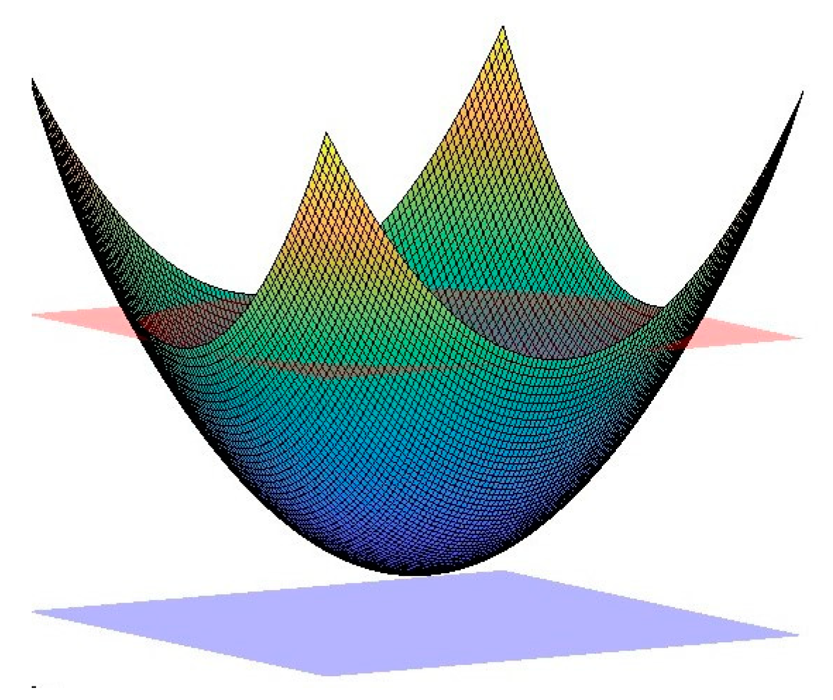
In this paper, the QP problem in standard form is solved by qpOASES [25] open source C++ library, and the extreme value of convex MPC [26] loss function is calculated considering its constraints. The process is shown in Figure 7, where the pink and blue parts represent the constraints, and an optimal set of control input is obtained within the constraints.
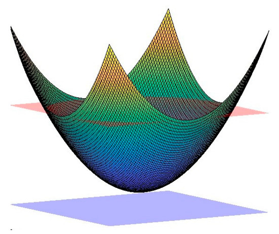
Figure 7.
QP optimization solution process.
4.4. Mapping of Joint Torque
In the multi-link model, the forward and inverse kinematics [27] is an extremely important link. The forward kinematics can carry out forward operations from the joint angle to the end position, and the inverse kinematics constructs the mapping from the joint angle to the end position and establishes the forward and inverse kinematics model of the biped robot system completely. The coordinate transformation of the Model-H16 robot used in this paper in Figure 8 obtained from the model measurement is shown in Table 2.
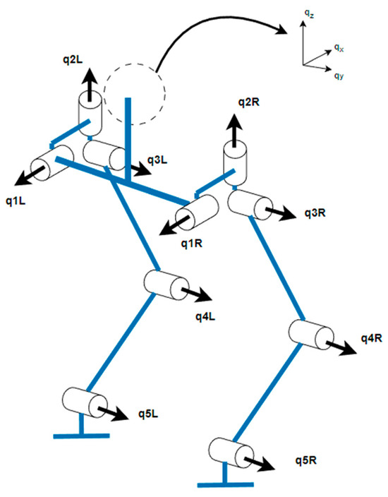
Figure 8.
The article-link model of a biped robot.
Table 2.
Motor coordinate transformation table.
According to the structure shown in Figure 8, this paper uses the improved D-H method to establish the D-H table of the system as shown in Table 3.
Table 3.
Table of D-H parameters.
The L1–L5 distribution in Table 3 represents the coordinate migration in 0, and – represents the joint rotation angle. The forward kinematic expression of the system can be easily calculated by the D-H parameters.
where, is the homogeneous transformation matrix from the center of mass to the foot end.
Through the position of the end in Equation (41), the linear velocity Jacobian matrix from the center of mass to the foot end can be calculated as Equation (42). Combined with the coordinate transformation of Equation (43), the obtained together constitute the velocity Jacobian of the system, and the velocity Jacobian matrix is shown in Equation (44).
where R is the rotation matrix from the center of mass to the end, .
The Jacobian matrix J I of the biped robot is obtained through Equation (44), which also means that we can directly calculate a set of joint torque through , such that the end position satisfies the MPC output in Equation (34). The joint torques of the supporting legs are calculated as shown in Equation (45).
5. Swing Leg Planning
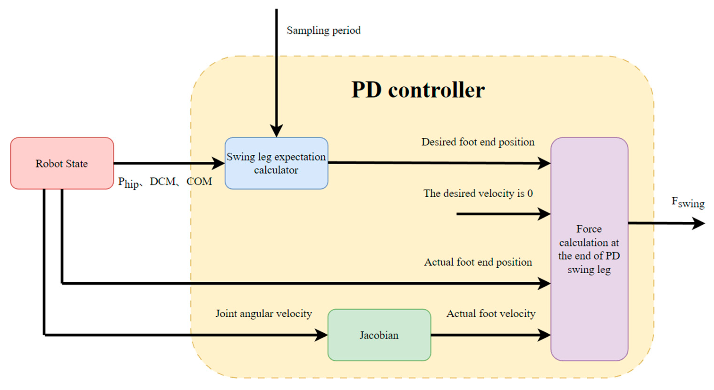
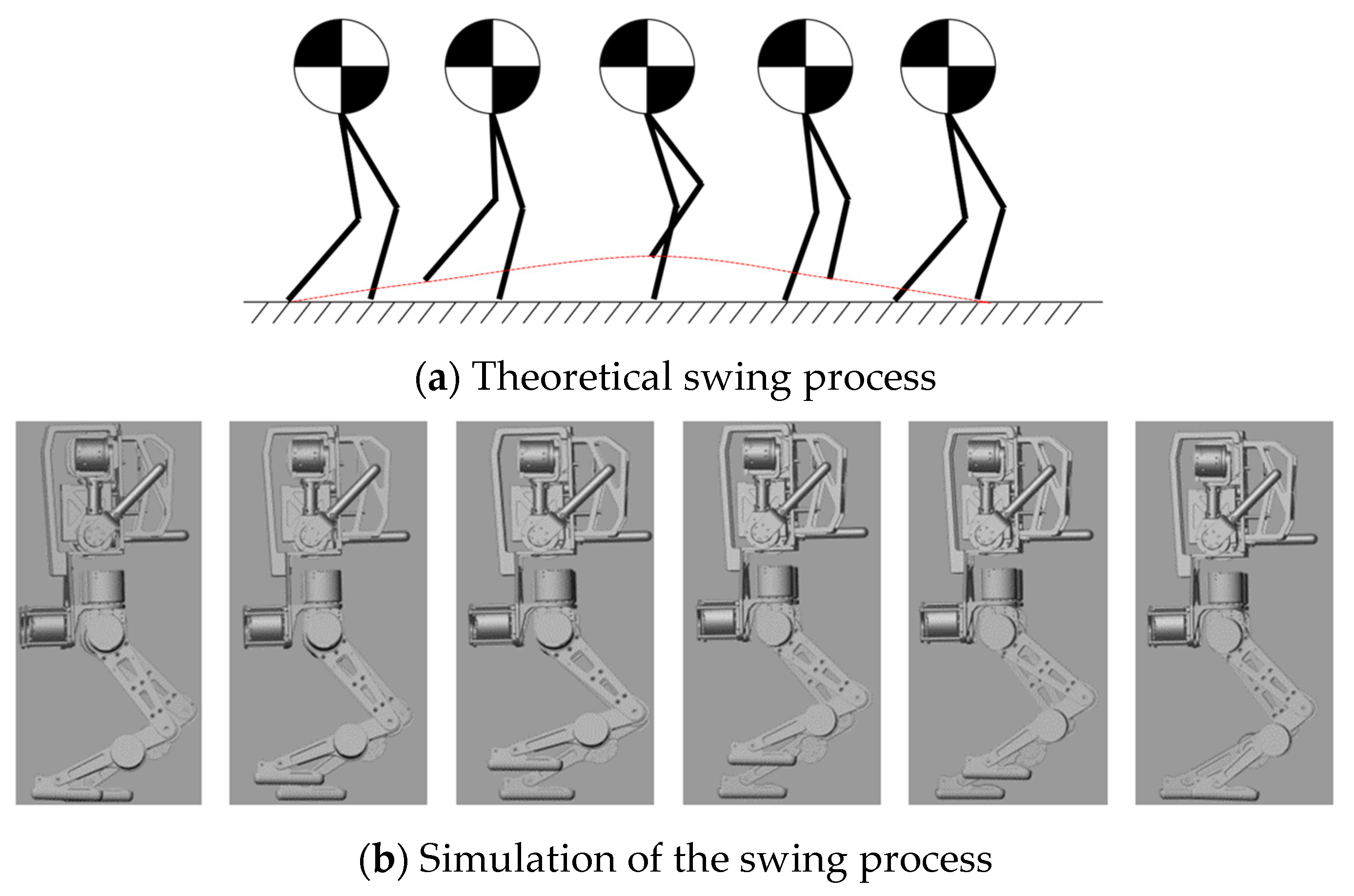
In the leg planning of biped robot, in addition to the support leg for maintaining balanced standing, another important part is the swing leg. Its role is to swing the swing leg at the end of the support cycle to the next position, and at the end of the half walking cycle (that is, half gait cycle), it falls to the next support position and is used as a new support leg. There are various gait planning methods for supporting legs, among which polynomial interpolation method [28] and PD control method [29] are typical. In this paper, the PD control method is used to control the swing leg, Figure 9 illustrates the structural diagram of the PD controller, the schematic diagram of the planned control result is shown in Figure 10a, the red curve in Figure 10a is the trajectory of the swinging leg, and the simulation swing process is shown in Figure 10b.

Figure 9.
The structure of the PD controller.
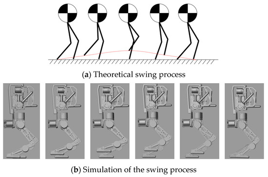
Figure 10.
Photo of the leg swing.
Because according to the PD control law, this paper focuses on the end force of the swing leg, and calculates according to the deviation of the speed of the swing leg end and the deviation of the position. Equation (46) calculates the expectation of the end position using the method from Carlo [30].
According to the Jacobian matrix in Equation (45), Equation (47) can calculate the velocity of the end through the joint angular velocity.
The actual foot position can be calculated from the actual position of the center of mass by forward kinematics, and is always kept as 0 in this paper to ensure continuity during movement. From the above four quantities, Equation (48) calculates the target force input at the foot end of the swing leg by means of PD.
6. Experimental Section
6.1. Simulation Experiment
In order to demonstrate the theoretical effect of the framework and algorithm, a series of experimental simulations were carried out on the Model-H16 robot based on MATLAB/Simulink (2023b) physical simulation environment, including uniform walking test, accelerated walking test, anti-interference ability test, and so on. At the same time, to facilitate the readers to better understand this part of the experiment, it is suggested to refer to the accompanying video: https://youtu.be/zabeuKK1_9U (accessed on 15 August 2024).
6.1.1. Constant-Speed Walking Test
In this part, the simulation test of constant-speed walking of the biped robot was designed, and the goal was to test the low-speed walking effect of the robot and the real-time trajectory of DCM. In this experiment, walking was carried out at a speed of 0.25 m/s, and its centroid and DCM real-time trajectory were shown in Figure 11. It can be seen that in the case of normal walking at low speed, the real-time DCM of the robot was basically approximately fitted to a straight line between the switching points, which represented that the linear constraint effect of DCM played a good role in MPC.
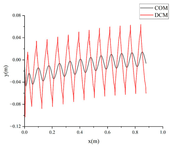
Figure 11.
COM and DCM trajectories for low-speed walking.
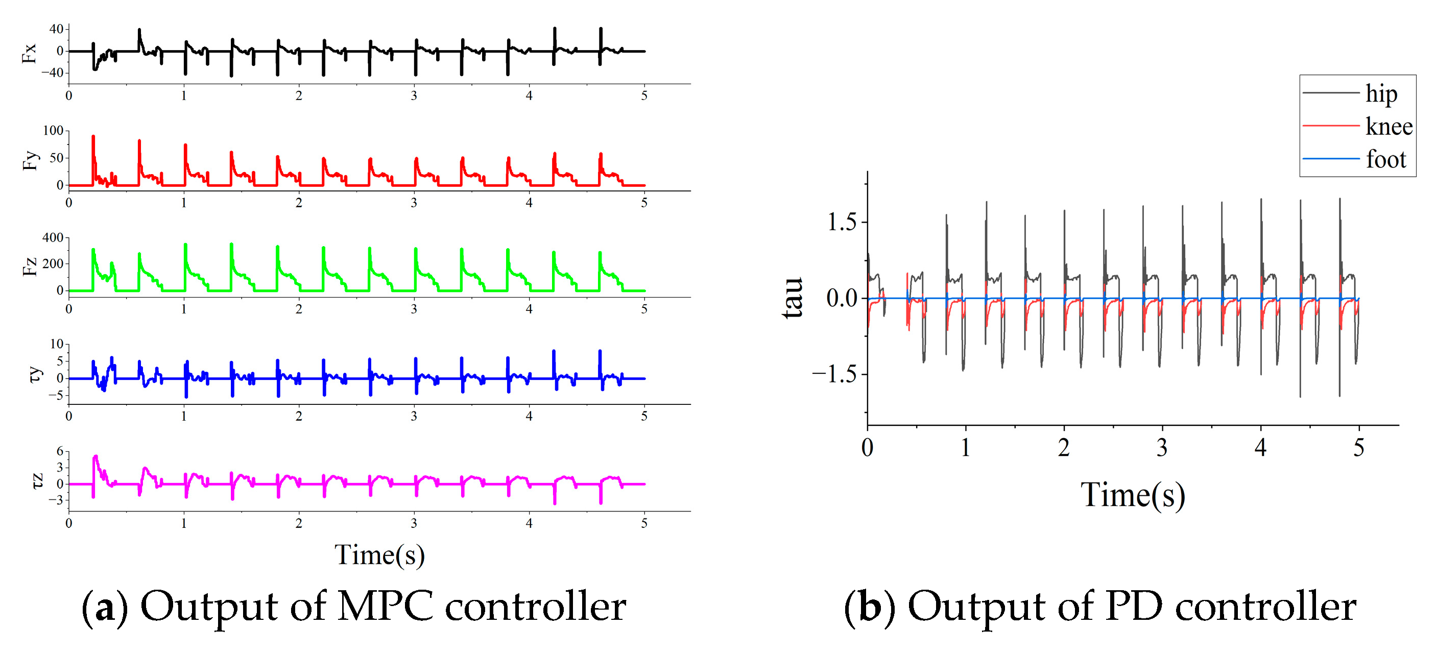
In order to show the effect of MPC and PD controller, Figure 12a shows the 3D force and 2D torque demand output by MPC during uniform walking. The figure shows that each time the left leg lands, large force and torque demand is generated to meet the needs of supporting the leg, where Fx and Fy fluctuate within 100 N, and Fz is under the demand of the normal force of the foot. The fluctuation range is within 400 N, which meets the requirement of 500 N constraint on the ground reaction force in this paper, and Fx, Fy, and Fz all show periodic laws during stable walking. The fluctuation range of torque is within 10 N and shows a stable and controlled trend.
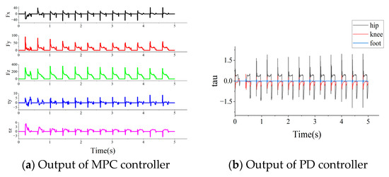
Figure 12.
COM and DCM trajectories for low-speed walking.
For the output effect of the PD controller, the output of the PD controller directly corresponded to the joint torques, and in this paper, the control torques of hip pitch, knee pitch, and ankle pitch are shown in Figure 12b. In each swing cycle, the torque at the moment of leg lift mutated to adapt to the position of the center of mass. During smooth walking, the output of the PD controller showed periodic changes, and the variation of the torque was within ±1.5 Nm.
6.1.2. Accelerated Walking Test
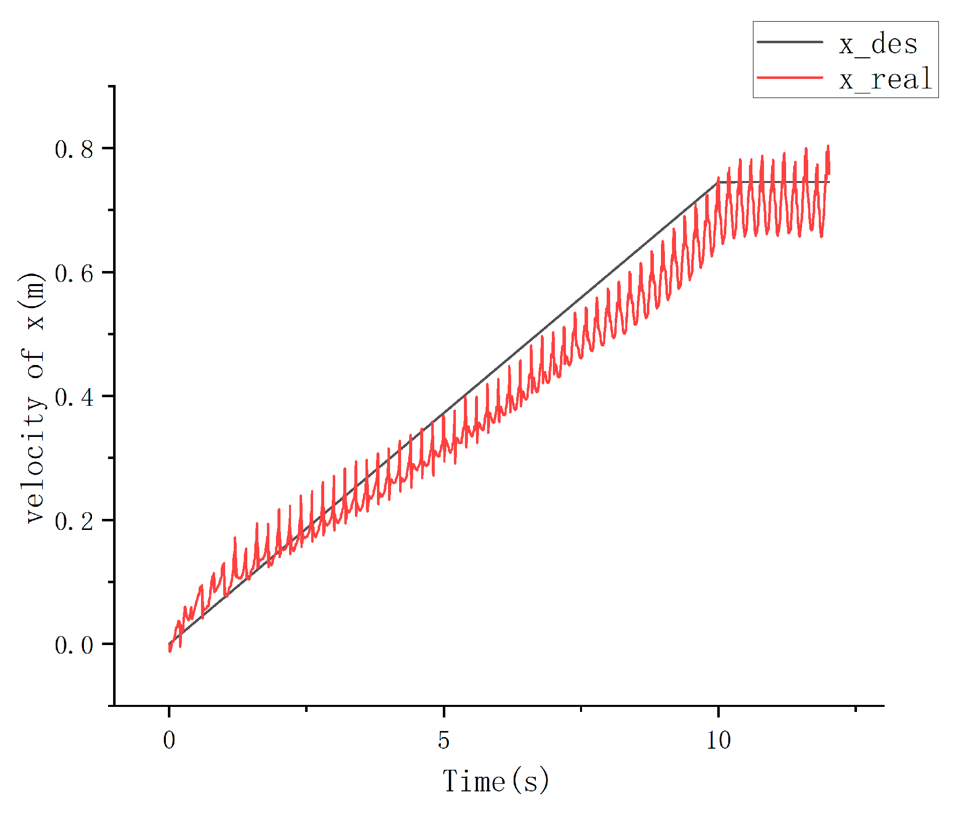
In order to verify the state effect of the algorithm under the maximum walking speed and acceleration of the Model-H16 robot, the acceleration walking test of the robot was carried out under the condition of flat terrain without interference. The test results of acceleration walking are shown in Figure 13 and Figure 14. Figure 13 shows the centroid tracking effect of the robot, and the robot shows good centroid tracking ability. In the figure, the maximum deviation between the actual centroid position and the target centroid position was 0.096 m/s, and the position repair can be completed after a certain time, and the robot can complete a good centroid following effect in normal walking. In this experiment, the robot reached a walking speed of 0.75 m/s. Considering that its leg length is only 0.3 m, the ratio of maximum speed to leg length was 2.5. Compared with Hector’s leg length of 0.44 m, the maximum speed of 1.1 m/s, and the ratio of maximum speed to leg length of 2.75, the robot can meet the needs of high-speed walking.
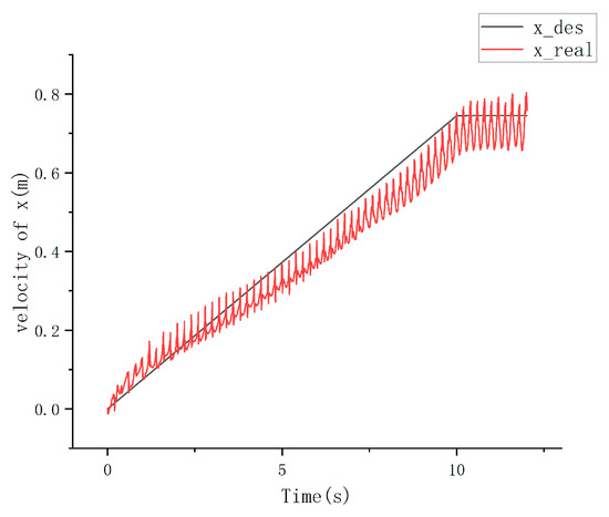
Figure 13.
Accelerate the x-direction velocity of the walking center of mass.
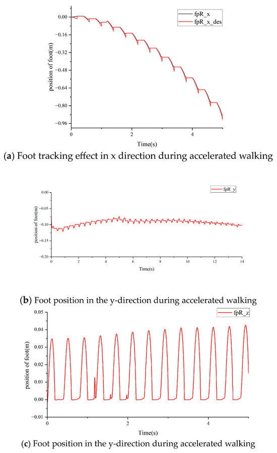
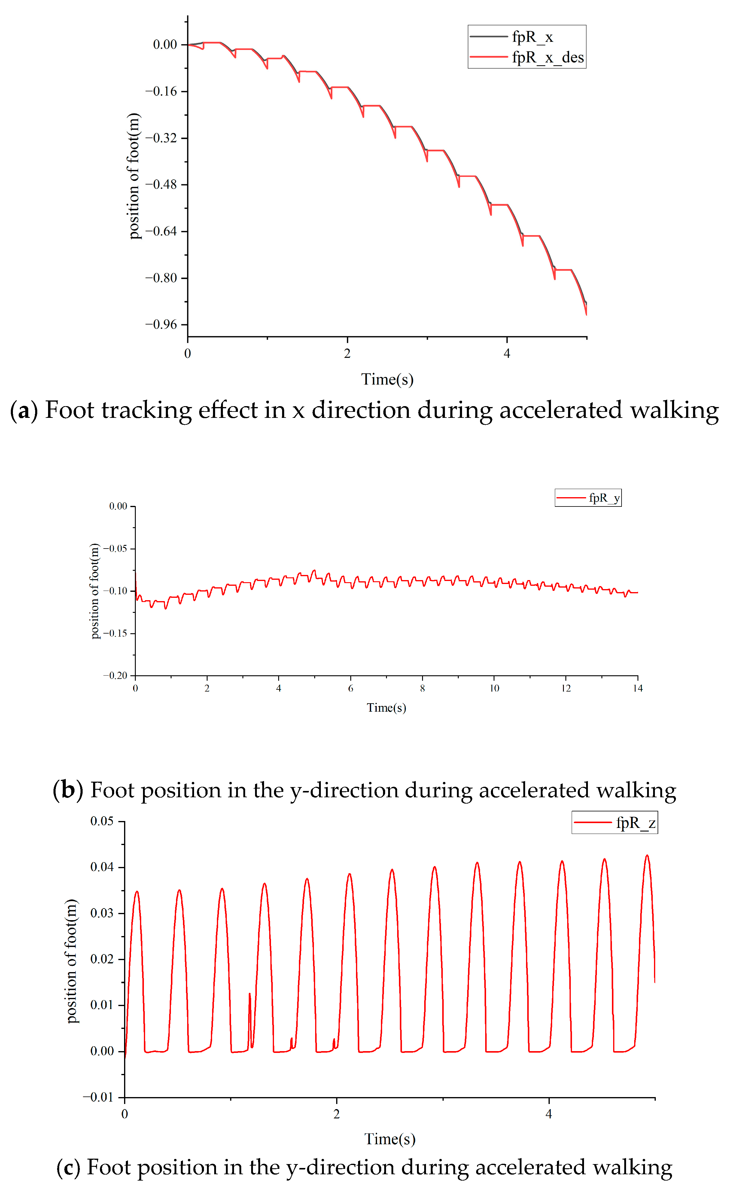
Figure 14.
Leg trajectory during walking.
At the same time, the position of the ends of both feet was also detected in the process of accelerated walking. Due to the symmetric nature of the left and right legs, only the right leg effect is shown in this part. Figure 14 shows the x, y, and z trajectories of the right foot. Figure 14a shows the target position and the actual position in the x direction. The error adjustment time was only 0.05 s, and the error of the landing position was approximately 0, which has a good tracking effect. Figure 14b shows the actual position in the y direction, which is basically around the standing position of −0.1 m during walking, and the deviation is within 0.03 m, which can meet the requirements of high-speed walking of the robot. Figure 14c shows the real-time walking position on the z-axis, whose lifted leg height approximately fluctuates at the set point of 0.3 m, and the half-step period is 0.2 s; that is, the left and right legs are switched every 0.2 s. In Figure 14c, the position of the foot end of the right leg is altered between 1–2 s due to accelerated walking. However, it was quickly repaired under the action of the controller, allowing it to return to the normal target tracking effect.
6.1.3. Anti-Jamming Capability Test
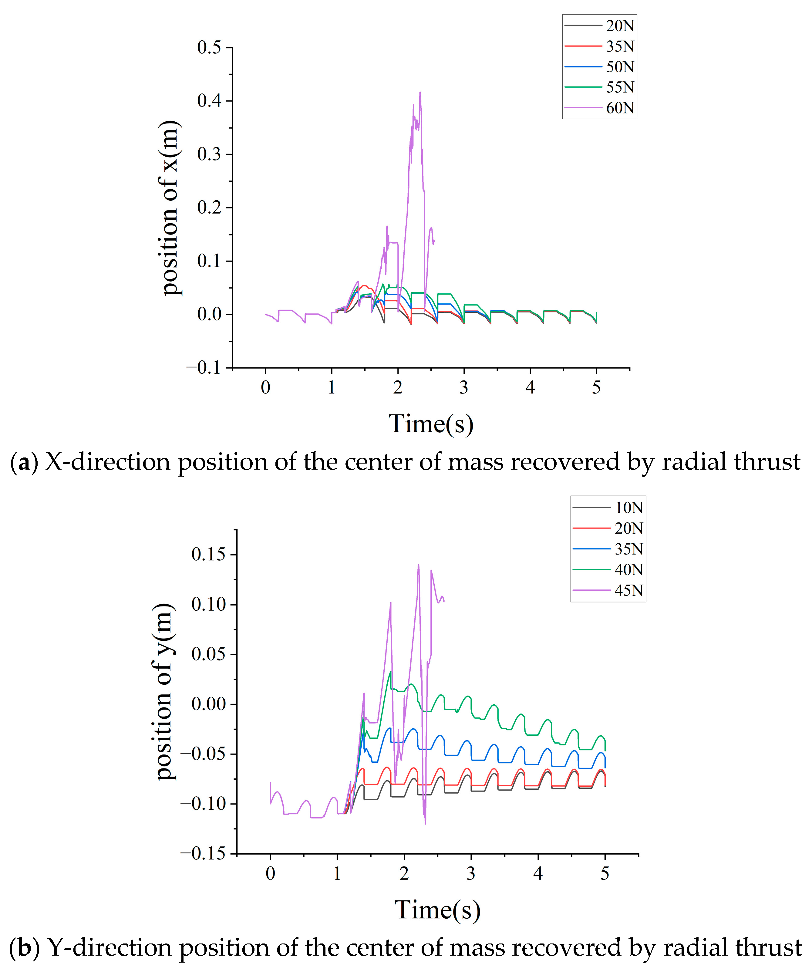
In order to verify the robustness and stability of the algorithm, this part applied an approximate impulse thrust with a duration of 0.2 s from the side and front of the robot at T = 1.0 s under the condition of the robot walking in place, imitated the external artificial thrust, broke the equilibrium state of the robot walking in place, and tested its maximum thrust recovery value. The test results are shown in Figure 15.
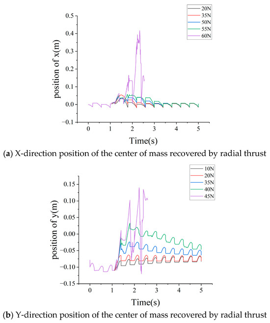
Figure 15.
Balance recovery effect under different disturbances in different directions.
In Figure 15a, the change in the radial direction (x-direction) of the centroid position of the robot is shown after a thrust of the same duration and different magnitude is applied to the lateral direction of the robot. In the experiment, the thrust from 20 N to 60 N was selected. The results show that 55 N thrust is the limit value of thrust recovery, and within the limit value, the offset in the radial direction of the robot is always less than 0.05 m. When the thrust increases to 60 N, the robot undergoes a large deviation (greater than 0.1 m) in the radial direction after 0.5 s of the thrust, resulting in the robot body flying and being unable to recover.
Figure 15b shows the lateral thrust effect, which is tested under the thrust of 10 N to 45 N, respectively. The test results show that when the thrust is small (10–20 N), the gait of the robot is almost not affected by the thrust, and the deviation of the center of mass in the y direction is less than 0.05 m. When the thrust increases from 20 N to 45 N, the robot exhibits a clear offset in the y direction, which is less than 0.1 m, and is recovered in the subsequent 2–5 s gait. When the thrust exceeds the limit value of 45 N, a large deviation (greater than 0.15 m) occurs in the y direction at 0.45 s after the thrust action. At this time, the lateral thrust makes the robot unable to recover the equilibrium state.
6.2. Physical Verification
In this paper, the algorithm was deployed on the Model-H16 robot to complete the basic walking function and obstacle crossing.
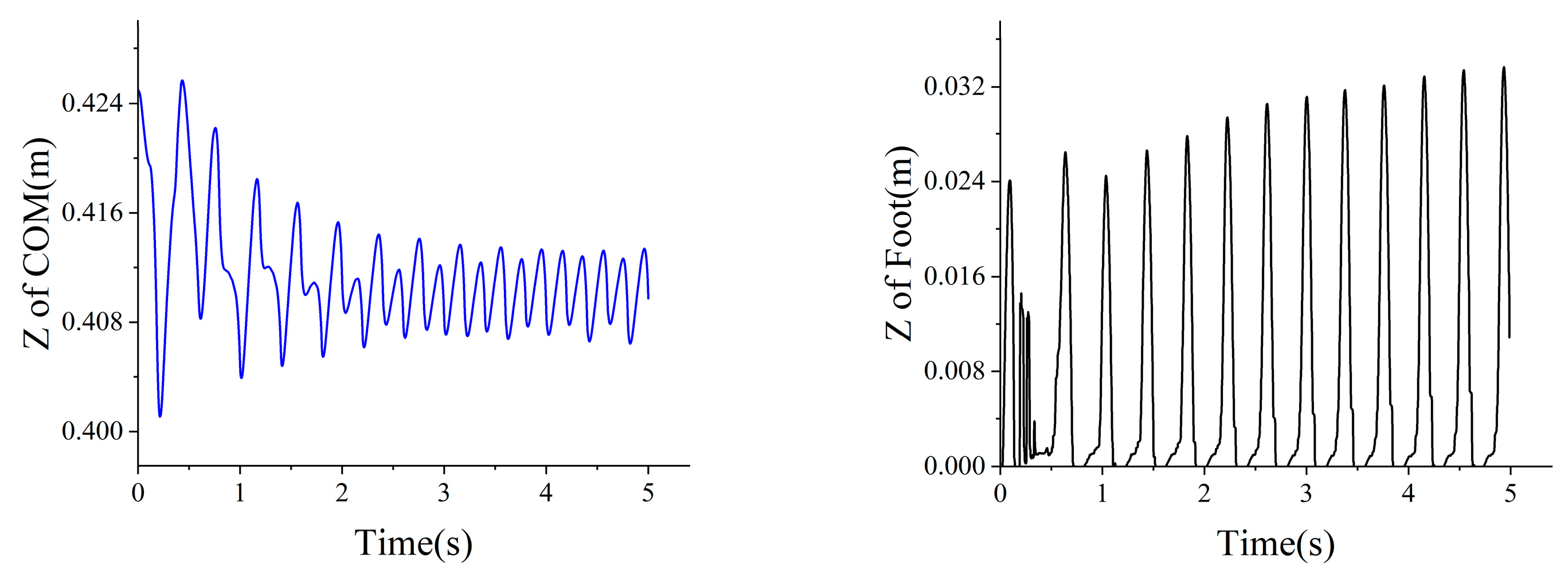
In the straight-line walking of the object, the right leg performed the action first and was used as the swing leg. After half a gait cycle (0.2 s), the swing leg and the support leg were exchanged, and the left leg was used as the swing leg. The continuous photo and centroid trajectory of the object were shown in Figure 16. In this paper, the Z-direction trajectory changes of the center of mass and the end of the right leg were collected in the process of uniform walking. Figure 17a shows the change of the height of the center of mass in the process of uniform walking. In the figure, the maximum deviation of the height of the center of mass in the 0–2 s gait is ±0.012 m and gradually tends to be stable, and the final position of the center of mass is constant at 4.15 ± 0.003 m. In the trajectory of the foot height, because the initial gait affected its balance, the gait was adjusted adaptively in the second gait cycle, and the foot height fluctuated in a small amplitude with high frequency. After one cycle of adjustment, normal walking was resumed, and the height and position of the center of mass were not affected. During normal walking, the foot height ranged from 0 to 0.03 m.
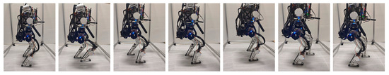
Figure 16.
Walking gait in a straight line was photographed.
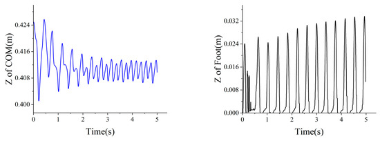
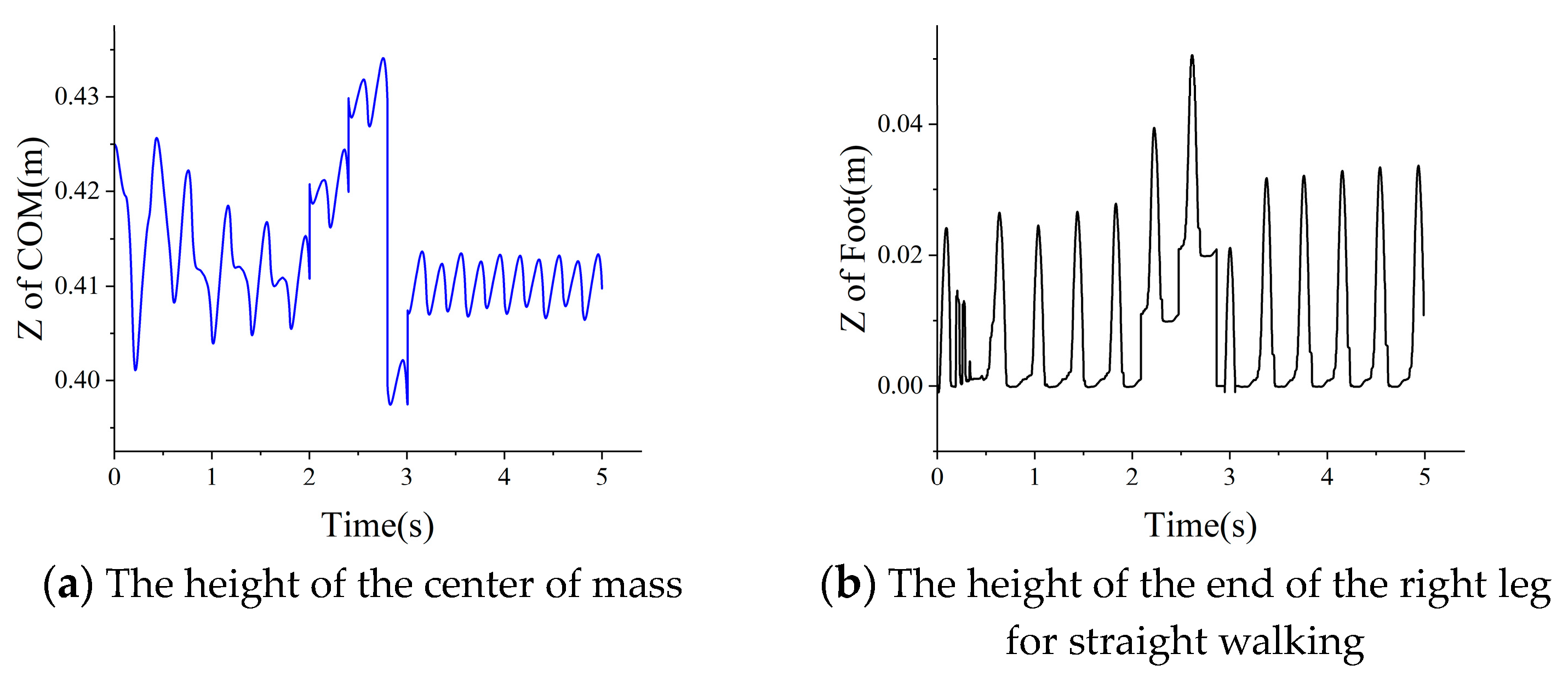
Figure 17.
Model-H16 linear walking center of mass and foot height. (a) The height of the center of mass. (b) The height of the end of the right leg for straight walking.
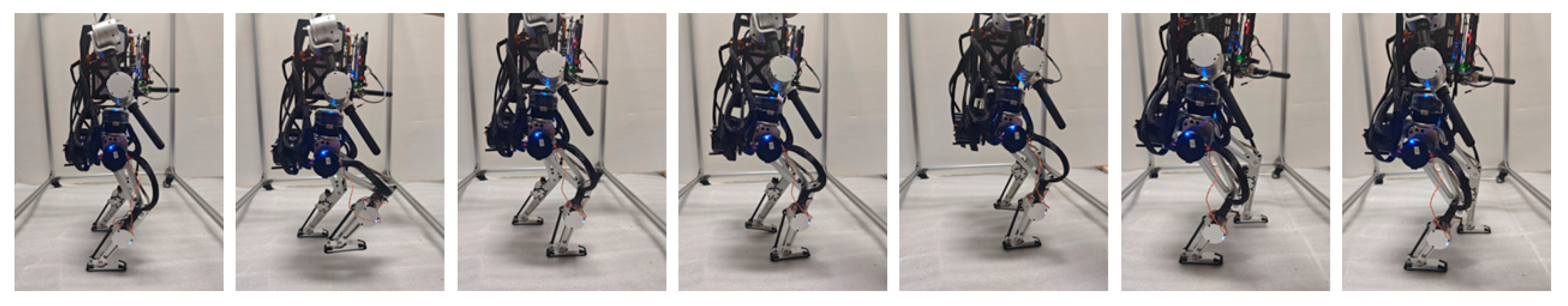
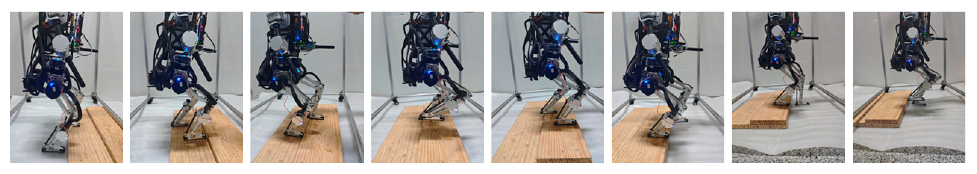
In the process of crossing the obstacle, the biped robot was able to successfully cross two levels of 10 mm wood boards and maintain balance during the crossing. Its physical photos are shown in Figure 18.

Figure 18.
Model-H16 walking and spanning gaits.
In the obstacle crossing test, the starting state was normal walking. When the gait was stable, the obstacle was encountered. The first stage of the board was crossed between 2–2.4 s, the second stage of the board was crossed between 2.4–2.8 s, and the landing buffer gait occurred between 2.8–3 s. As shown in Figure 19, the height of the center of mass fluctuates from 0.41 m to 0.42 m, then to 0.43 m, and finally changes to 0.41 m upon landing. The position of the foot end of the right foot changed from 0 to 0.02 m, and finally the normal walking state was restored by a half gait of 0.2 s.
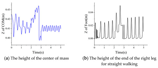
Figure 19.
The Model-H16 spans the walking center of mass and foot height.
7. Discussion and Conclusions
Through a series of experiments in Section 6, this paper shows the control effect of the proposed algorithm for the general forward flexion type 10-degree-of-freedom biped robot and also proves the excellent performance of the DCM-MPC control method in velocity following and disturbance resistance. This will extend the application of DCM in the field of biped robots, incorporating not only Englsberger’s [10] work and its related derivative theory but also considering the concept of multi-model fusion as proposed by Zhang Zhao [15]. Compared with the research of Englsberger [11], this paper simplifies the process of dynamic modeling, combines LIPM with simplified rigid body dynamics for modeling, and introduces the control method of force and torque, which is more universal for 10 DOF robots. Moreover, the control target becomes 10 DOF underactuated robots, so the research is more challenging. Compared with the research results of Li [19], this paper does not directly use the complete state of the center of mass for consideration but introduces the variable DCM. This approach not only considers the state of the center of mass but also makes it more convenient for MPC to constrain and optimize the trajectory of DCM, providing a more intuitive to analyze the stability and optimize the trajectory of the robot. When MPC constraints are considered, the linear foot constraints are consistent with Caron’s [23] algorithm and the friction cone is expanded in the two-dimensional plane x-z, and the toe and heel are constrained, respectively. Another feature of constraint in this paper is that DCM is transformed from control target to control constraint. Compared with Hopkins [16] and Griffin [17], perfect leg force, torque, friction cone, and DCM constraints are established in this paper. Although the speed of the algorithm is close to that of the Hector robot, and it has good anti-disturbance ability in radial and lateral directions, the effect of the concave and convex terrain of the ground still needs to be improved.
In summary, this paper proposes a new control framework based on the force and torque control framework, combined with DCM theory to establish the control model. Each constraint adjustment, such as line angle, friction cone, force and torque, and new DCM constraint, is introduced to establish the MPC control strategy. The program library qpOASES is used to solve the quadratic programming problem in MPC, and the PD control method is used to complete the control of the swing leg. Finally, the robot control system is completely realized by mapping the torque Jacobian to the joint motor. In the simulation experiments, this paper demonstrates that the DCM trajectory maintains a straight line in the gait, the control algorithm achieves a fast walking of 0.75 m/s on the Model-H16 robot, and the velocity deviation remains below 0.096 m/s in the velocity tracking process. Additionally, it shows the robot’s anti-disturbance ability in both the radial and lateral directions. In the physical experiment, the ability of the robot to walk in place and pass through the obstacle at low speed is demonstrated, which also verifies the effectiveness of the proposed algorithm in the physical deployment and migration. The follow-up work will focus on the realization of high-speed walking of the physical robot and achieve a breakthrough in the algorithm framework.
Author Contributions
Conceptualization, Z.W. and Z.F.; methodology, Z.W. and W.D.; software, Z.W.; validation, Z.W., Z.F., T.W. and X.H.; formal analysis, Z.W., Z.F. and W.D.; investigation, Z.W. and X.H.; resources, Z.F., W.D. and X.H.; data curation, Z.W.; writing—original draft preparation, Z.W.; writing—review and editing, Z.W.; visualization, Z.W.; supervision, Z.W. All authors have read and agreed to the published version of the manuscript.
Funding
This research received no external funding.
Data Availability Statement
Data are contained within the article.
Conflicts of Interest
The authors declare no conflict of interest.
References
- Lim, H.-O.; Takanishi, A. Biped walking robots created at Waseda University: WL and WABIAN family. Philos. Trans. R. Soc. A Math. Phys. Eng. Sci. 2007, 365, 49–64. [Google Scholar] [CrossRef] [PubMed]
- Zhang, Y.; Arakelian, V. Legged walking robots: Design concepts and functional particularities. In Advanced Technologies in Robotics and Intelligent Systems: Proceedings of ITR 2019; Springer International Publishing: Cham, Switzerland, 2020; pp. 13–23. [Google Scholar]
- Vukobratović, M.; Stepanenko, J. On the stability of anthropomorphic systems. Math. Biosci. 1972, 15, 1–37. [Google Scholar] [CrossRef]
- Caron, S.; Escande, A.; Lanari, L.; Mallein, B. Capturability-based pattern generation for walking with variable height. IEEE Trans. Robot. 2019, 36, 517–536. [Google Scholar] [CrossRef]
- Guan, K.; Yamamoto, K.; Nakamura, Y. Virtual-mass-ellipsoid inverted pendulum model and its applications to 3D bipedal locomotion on uneven terrains. In Proceedings of the 2019 IEEE/RSJ International Conference on Intelligent Robots and Systems (IROS), Macau, China, 3–8 November 2019; IEEE: Piscataway, NJ, USA, 2019. [Google Scholar]
- Li, W.; Li, L.; Zhou, L.; Zhuang, Z.; Chen, Y. Climbing Stairs Gait Planning and Virtual Simulation for Biped Robot Based on Three-Dimensional Inversed Pendulum. In Proceedings of the 2022 7th International Conference on Robotics and Automation Engineering (ICRAE), Singapore, 18–20 November 2022; IEEE: Piscataway, NJ, USA, 2022. [Google Scholar]
- Pratt, J.; Krupp, B. Design of a bipedal walking robot. In Proceedings of the SPIE Defense and Security Symposium, Orlando, FL, USA, 16–20 March 2008; Unmanned Systems Technology X. SPIE: Bellingham, WA, USA, 2008; Volume 6962. [Google Scholar]
- Kajita, S.; Kanehiro, F.; Kaneko, K.; Fujiwara, K.; Harada, K.; Yokoi, K.; Hirukawa, H. Biped walking pattern generation by using preview control of zero-moment point. In Proceedings of the 2003 IEEE International Conference on Robotics and Automation (Cat. No. 03CH37422), Taipei, Taiwan, 14–19 September 2003; IEEE: Piscataway, NJ, USA, 2003; Volume 2. [Google Scholar]
- Takenaka, T.; Matsumoto, T.; Yoshiike, T. Real time motion generation and control for biped robot -1st report: Walking gait pattern generation. In Proceedings of the 2009 IEEE/RSJ International Conference on Intelligent Robots and Systems, St. Louis, MO, USA, 10–15 October 2009; IEEE: Piscataway, NJ, USA, 2009. [Google Scholar]
- Englsberger, J.; Ott, C.; Albu-Schaffer, A. Three-dimensional bipedal walking control using divergent component of motion. In Proceedings of the 2013 IEEE/RSJ International Conference on Intelligent Robots and Systems, Tokyo, Japan, 3–7 November 2013; IEEE: Piscataway, NJ, USA, 2013. [Google Scholar]
- Englsberger, J.; Ott, C.; Roa, M.A.; Albu-Schäffer, A.; Hirzinger, G. Bipedal walking control based on capture point dynamics. In Proceedings of the 2011 IEEE/RSJ International Conference on Intelligent Robots and Systems, San Francisco, CA, USA, 25–30 September 2011; IEEE: Piscataway, NJ, USA, 2011. [Google Scholar]
- Kim, S.-H.; Hong, Y.-D. Dynamic bipedal walking using real-time optimization of center of mass motion and capture point-based stability controller. J. Intell. Robot. Syst. 2021, 103, 58. [Google Scholar] [CrossRef]
- Han, L.; Chen, X.; Yu, Z.; Zhang, J.; Gao, Z.; Huang, Q. Enhancing speed recovery rapidity in bipedal walking with limited foot area using DCM predictions. Expert Syst. Appl. 2024, 250, 123858. [Google Scholar] [CrossRef]
- Morisawa, M.; Kajita, S.; Kanehiro, F.; Kaneko, K.; Miura, K.; Yokoi, K. Balance control based on capture point error compensation for biped walking on uneven terrain. In Proceedings of the 2012 12th IEEE-RAS International Conference on Humanoid Robots (Humanoids 2012), Osaka, Japan, 7 November 2013; IEEE: Piscataway, NJ, USA, 2012. [Google Scholar]
- Zhang, Z.; Zhang, L.; Xin, S. Machine Vision-based Recognition and Positioning System for Domestic Garbage. In Proceedings of the 2021 IEEE International Conference on Robotics and Biomimetics (ROBIO), Sanya, China, 27–31 December 2021; IEEE: Piscataway, NJ, USA, 2021; pp. 1559–1563. [Google Scholar]
- Hopkins, M.A.; Hong, D.W.; Leonessa, A. Humanoid locomotion on uneven terrain using the time-varying divergent component of motion. In Proceedings of the 2014 IEEE-RAS International Conference on Humanoid Robots, Madrid, Spain, 18–20 November 2014; IEEE: Piscataway, NJ, USA, 2014. [Google Scholar]
- Griffin, R.J.; Leonessa, A. Model predictive control for dynamic footstep adjustment using the divergent component of motion. In Proceedings of the 2016 IEEE International Conference on Robotics and Automation (ICRA), Stockholm, Sweden, 16–21 May 2016; IEEE: Piscataway, NJ, USA, 2016. [Google Scholar]
- Ugurlu, B.; Saglia, J.A.; Tsagarakis, N.G.; Caldwell, D.G. Hopping at the resonance frequency: A trajectory generation technique for bipedal robots with elastic joints. In Proceedings of the 2012 IEEE International Conference on Robotics and Automation 2012, Saint Paul, MN, USA, 14–18 May 2012; pp. 1436–1443. [Google Scholar]
- Li, J.; Nguyen, Q. Force-and-moment-based Model Predictive Control for Achieving Highly Dynamic Locomotion on Bipedal Robots. In Proceedings of the 2021 60th IEEE Conference on Decision and Control (CDC), Austin, TX, USA, 14–17 December 2021; pp. 1024–1030. [Google Scholar]
- Ding, B.; Yang, Y. Model Predictive Control; John Wiley & Sons: Hoboken, NJ, USA, 2024. [Google Scholar]
- Rawlings, J.B.; Mayne, D.Q.; Diehl, M. Model Predictive Control: Theory, Computation, and Design; Nob Hill Publishing: Madison, WI, USA, 2017; Volume 2. [Google Scholar]
- Carpentier, J.; Saurel, M.; Tonneau, S.; Stasse, O.; Mansard, N. Quadratic Programming for Multi-Contact Planning and Control of Humanoid Robots. IEEE Trans. Robot. 2018, 34, 370–382. [Google Scholar]
- Caron, S.; Pham, Q.-C.; Nakamura, Y. Stability of surface contacts for humanoid robots: Closed-form formulae of the contact wrench cone for rectangular support areas. In Proceedings of the 2015 IEEE International Conference on Robotics and Automation (ICRA), Seattle, WA, USA, 26–30 May 2015; IEEE: Piscataway, NJ, USA, 2015. [Google Scholar]
- Wei, Z.; Deng, W.; Feng, Z.; Huang, X. Offline Walking Strategy Of Biped Robot Based On Improved DCM. In Proceedings of the 2023 5th International Academic Exchange Conference on Science and Technology Innovation (IAECST), Guangzhou, China, 8–10 December 2023; IEEE: Piscataway, NJ, USA, 2023. [Google Scholar]
- Raffo, G.V.; Ortega, M.G.; Rubio, F.R. An integral predictive/nonlinear H∞ control structure for a quadrotor helicopter. Automatica 2010, 46, 29–39. [Google Scholar] [CrossRef]
- Ferreau, H.J.; Kirches, C.; Potschka, A.; Bock, H.G.; Diehl, M. qpOASES: A parametric active-set algorithm for quadratic programming. Math. Program. Comput. 2014, 6, 327–363. [Google Scholar] [CrossRef]
- Ye, H.; Wang, D.; Wu, J.; Yue, Y.; Zhou, Y. Forward and inverse kinematics of a 5-DOF hybrid robot for composite material machining. Robot. Comput.-Integr. Manuf. 2020, 65, 101961. [Google Scholar] [CrossRef]
- Lu, Y.; Tian, X.; Jiang, H.; You, T.; Han, J.; Xia, L. A flexible topological flank modification method based on polynomial interpolation function. J. Adv. Mech. Des. Syst. Manuf. 2023, 17, JAMDSM0041. [Google Scholar] [CrossRef]
- Siciliano, B.; Sciavicco, L.; Villani, L.; Oriolo, G. Trajectory Planning. In Robotics (Modeling, Planning and Control); Springer: Berlin/Heidelberg, Germany, 2010; pp. 161–189. [Google Scholar]
- Di Carlo, J.; Wensing, P.M.; Katz, B.; Bledt, G.; Kim, S. Dynamic locomotion in the MIT cheetah 3 through convex model-predictive control. In Proceedings of the 2018 IEEE/RSJ International Conference on Intelligent Robots and Systems (IROS), Madrid, Spain, 1–5 October 2018; IEEE: Piscataway, NJ, USA, 2018. [Google Scholar]


Disclaimer/Publisher’s Note: The statements, opinions and data contained in all publications are solely those of the individual author(s) and contributor(s) and not of MDPI and/or the editor(s). MDPI and/or the editor(s) disclaim responsibility for any injury to people or property resulting from any ideas, methods, instructions or products referred to in the content. |
© 2024 by the authors. Licensee MDPI, Basel, Switzerland. This article is an open access article distributed under the terms and conditions of the Creative Commons Attribution (CC BY) license (https://creativecommons.org/licenses/by/4.0/).