Abstract
In order to solve the problem of autonomous vehicles driving safely on the road while searching for optimal paths to avoid traffic congestion and obstruction, this paper establishes an optimal path planning model based on image feature extraction. The model consists of four parts: the selection of key turning points, interpolation between turning points, definition of the evaluation function, and global optimal path search. First, based on the map information provided by the network, an image feature detection algorithm was proposed, and the key turning points of the map route were selected and stored in an open table. Then, based on mechanical analysis theory, the cubic interpolation between two key turning points of the optimal path was defined. This allows the car to drive along a continuous curve with a certain arc radius, enabling it to drive smoothly, effectively avoid obstacles, and ensure safety. Then, an evaluation function is defined as needed, and different evaluation functions are specified for different road sections to avoid excessive local deviations in planning and to reduce the impact of known obstacles on the path. Finally, the cost of the search path is calculated based on the evaluation function. According to the principle of minimum cost, a globally optimal heuristic search algorithm is proposed to find the globally optimal path. Experimental results show that the proposed global optimal path planning algorithm has excellent performance, with an average accuracy of 96.71% and a search speed of 2.78 ms. The model not only provides accurate path planning and fast path selection capabilities but also has strong robustness against interference.
1. Introduction
With the rapid development of economy and society, urban traffic congestion is becoming more and more serious, especially in some megacities, where road congestion, blockage and traffic accidents are common. Then, autonomous vehicles need accurate, safe, and reasonable navigation to avoid traffic jams and reduce the incidence of accidents. It is necessary to install a real-time path planning system on autonomous vehicles. This system must have optimized computation, accurate navigation, and a global optimal path planning function for fast positioning. Therefore, it is urgent to study the optimal path planning method of autonomous vehicles, which has important theoretical value and practical significance.
In recent years, path planning has attracted extensive attention in the fields of autonomous driving, logistics distribution, and robot navigation. To better understand the current state of related research, we review the existing literature and summarize their respective advantages and disadvantages, as shown in Table 1.

Table 1.
Advantages and disadvantages of previous path planning algorithms.
Wu et al. [1] established a road intersection control model based on mixed integer linear programming, which reduced the delay time of autonomous driving vehicles and improved space utilization efficiency. However, this method may have computational complexity for real-time applications and does not consider the mixed traffic of human-driven vehicles. Fan et al. [2] designed an adaptive variable neighborhood cultural gene algorithm for the path planning problem under the multi-center joint distribution model, which effectively solved the problem of random demand matching, but the computational complexity was high and may not be suitable for ultra-large-scale problems. Genetic algorithms (GAs) and evolutionary algorithms are widely used in the field of path planning as global optimization tools due to their powerful search capabilities and adaptability. However, these algorithms have high computational complexity, may converge slowly, and are sensitive to parameter settings, which may not be suitable for ultra-large-scale problems [24].
To address this problem, Lin et al. [22] proposed a hybrid particle swarm optimization and simulated annealing (PSO-SA) algorithm to optimize the path planning of automatically guided vehicles (AGVs). In comparing with other heuristic algorithms (including the harmony search algorithm, firefly algorithm, artificial bee colony algorithm, and genetic algorithm), the algorithm performed well in handling optimization problems. It reduces the possibility of falling into the local optimum, improves the efficiency of obtaining the global optimal solution, converges faster, and consumes less time. Similarly, Shi et al. [21] proposed an improved simulated annealing (SA) dynamic path planning algorithm. By introducing the initial path selection method and deletion operation, the computational workload is reduced. Simulation results show that the improved SA algorithm is superior to other algorithms and provides optimal solutions in static and dynamic environments.
Li et al. [3] proposed a hybrid path planning algorithm combining the A* and dynamic window algorithms (DWA), which improved the path finding speed and obstacle avoidance ability of the mobile robot, but the implementation complexity is high and may depend on the characteristics of the environment. Li et al. [4] improved the Dijkstra algorithm, taking into account a variety of traffic factors, and improved the navigation accuracy and speed, but the quantification of each factor is more complicated and requires real-time data support. In addition, Li et al. [5] proposed an improved A algorithm based on a heuristic search strategy to improve the path quality and path finding efficiency.
In order to solve the problems of too many redundant nodes, long search time, and sharp turns in the traditional A algorithm, Han et al. [19] proposed a five-neighborhood search A algorithm that adds dynamic weighting to the heuristic function and uses second-order Bezier curves for path smoothing. Simulation results show that compared with the traditional eight-neighborhood search algorithm, the number of redundant nodes and search time of the improved algorithm are reduced by 86.57% and 82.07%, respectively, and the cost remains unchanged under high precision. After Bezier curve processing, the obtained path has no large-angle turning points. After smooth optimization, the continuity of speed and acceleration can be maintained, which improves driving smoothness.
Liu et al. [6] proposed a bat algorithm with reverse learning and a tangent random exploration mechanism, which improves global and local search capabilities, but the algorithm complexity is high and parameter adjustment is difficult. To solve the global optimal problem in path planning, Ding et al. [23] proposed an extended path RRT* (EP-RRT*) algorithm based on the heuristic sampling of the path extension area. The algorithm combines the greedy heuristic strategy of Rapid Exploration Random Tree (RRT)-Connect to quickly explore the environment to find a feasible path, and then expands the path to obtain a heuristic sampling area. An iterative search is performed in this area. As the path is optimized, the sampling area changes continuously, and finally, the optimal or suboptimal path connecting the starting point and the target point is obtained.
In terms of path planning in marine environments, Hu et al. [7] proposed a real-time path planning algorithm that uses marine radar to detect obstacles in real time and achieves obstacle avoidance for high-speed ships. However, this method mainly targets static obstacles and relies on the quality of radar data. In response to the connection and disconnection problems of autonomous vehicles on multi-lane highways, Babu et al. [20] developed a new path planning method. The objective function of this method includes factors such as vehicle performance improvement, passenger comfort, vehicle collision prevention, and road deviation avoidance. The Hunger Game Improved Archimedean Optimization Algorithm (HGE-ARCO) is used for path optimization. In 100 trials, the maximum speed of the HGE-ARCO scheme reached about 99 km/h and took 12.3021 s, which is better than other conventional methods.
In the field of Uncrewed Aerial Vehicle (UAV) path planning, Li et al. [8] designed an auxiliary collision avoidance system based on machine vision, which has high-precision obstacle avoidance capabilities, but may be limited in complex urban environments. Zhang et al. [9] studied the obstacle avoidance path planning method of power grid inspection robots, combining global and local methods to effectively avoid static and dynamic obstacles, but there may be local minimum problems. In the field of electric vehicle path planning, Xing et al. [10] proposed a path planning and charging navigation strategy based on real-time traffic information, taking into account the impact of electric vehicles on the power grid, but accurate real-time traffic data are required.
Other studies include path planning methods based on Linear Temporal Logic (LTL) [11], underground vehicle path planning based on genetic algorithms [12], and energy-optimal trajectory planning for two-wheeled self-balancing robots [13]. These methods have achieved good results in their respective fields, but they also have some limitations. Fu et al. [14], Li et al. [15], Nahum et al. [16], Yin et al. [17], Avola et al. [18], etc., have proposed innovative research results in vehicle synchronous transfer, keyword-aware routing, multi-target evacuation model, path coverage algorithms, and drone continuous monitoring.
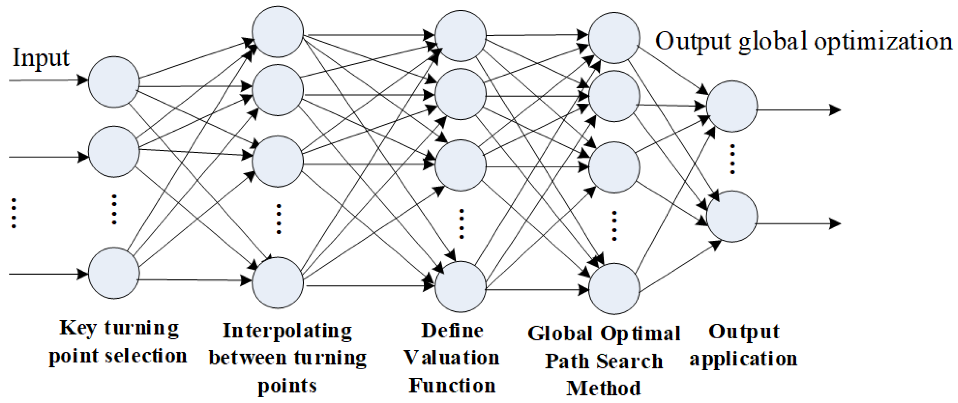
In order to enable the navigation and positioning system to continue to provide reliable services and to reduce the safety hazards caused by improper path planning, this paper proposes a global path optimal planning model. The model is divided into four parts as shown in Figure 1, where each node represents a different method used under different conditions. The first is to provide an image feature extraction method for the map to extract the major turning points of the path. The second is to perform a three-dimensional interpolation algorithm between the major turning points to make the car drive at a balanced, safe, and reasonable speed. The third part is to analyze road conditions—such as congestion—to minimize driving time, fuel consumption, or distance by providing an evaluation function for route change decisions. The cost function can be defined in sections to avoid excessive deviation in local planning and to reduce the impact of known obstacles on the path. The fourth part is to provide a heuristic path search algorithm based on the cost function to search for the optimal path. Finally, experiments were conducted on uncrewed vehicles to verify the feasibility and effectiveness of the model established in this paper and compare the model with existing optimal path planning algorithms. The comparison results show that the optimal path planning method proposed in this paper outperforms existing algorithms due to its more accurate path selection, faster path determination, and strong anti-interference ability. Its strong anti-interference ability stems from the evaluation function and the global optimal search algorithm being unaffected by external signals.
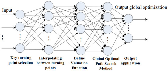
Figure 1.
Global path optimal planning model.
The contributions of this study are summarized as follows: (1) A global path optimal planning model is proposed, which enables the navigation and positioning system to continuously provide reliable services and reduce the safety hazards caused by improper path planning. (2) A map image feature extraction method is proposed to extract the key turning points of the path. Interpolation is performed between key turning points to smooth the vehicle trajectory. A cost function was designed, and a heuristic path search algorithm was proposed to search for the optimal path. (3) The experimental results show that the global path optimal planning algorithm proposed in this paper performs well, with an average accuracy of 96.71% and a search time of 2.78 ms.
2. Overview
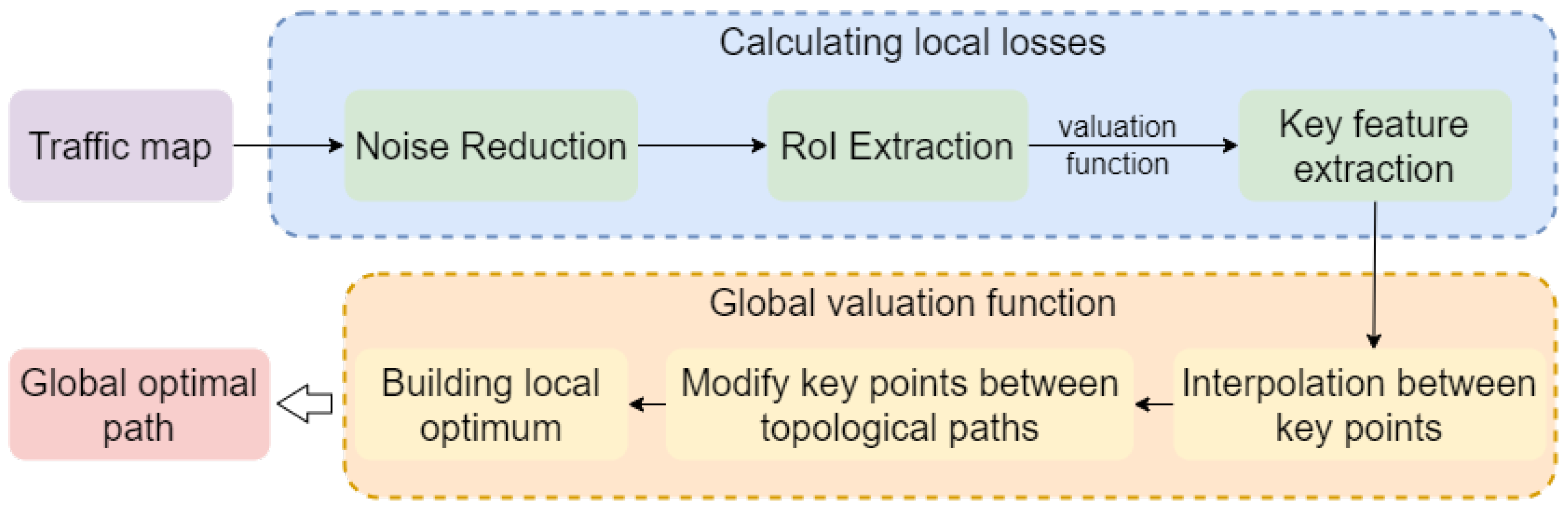
The overall pipeline of the proposed method is shown in Figure 2. Initially, the traffic map undergoes denoising to remove redundant information. Next, key areas within the traffic map are identified, and the local loss in each area is calculated to extract key points (i.e., road intersections). To address potential discontinuities between these key points, topological interpolation is applied to generate a smooth, locally optimal path. Finally, the key points are further refined and supplemented through a global valuation function, ensuring optimal decisions at each road intersection and thereby achieving a globally optimal path.
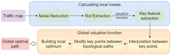
Figure 2.
The pipeline of the proposed global path optimal planning method.
3. Key Turning Point Selection Method
In scenarios involving intersections across multiple roads, accurately determining the location of these intersections and the direction of each road is crucial for optimal path selection. The “key turning point selection method” offers an effective approach for identifying these pivotal points, thereby supporting subsequent path planning decisions.
3.1. Region of Interest (ROI) Extraction
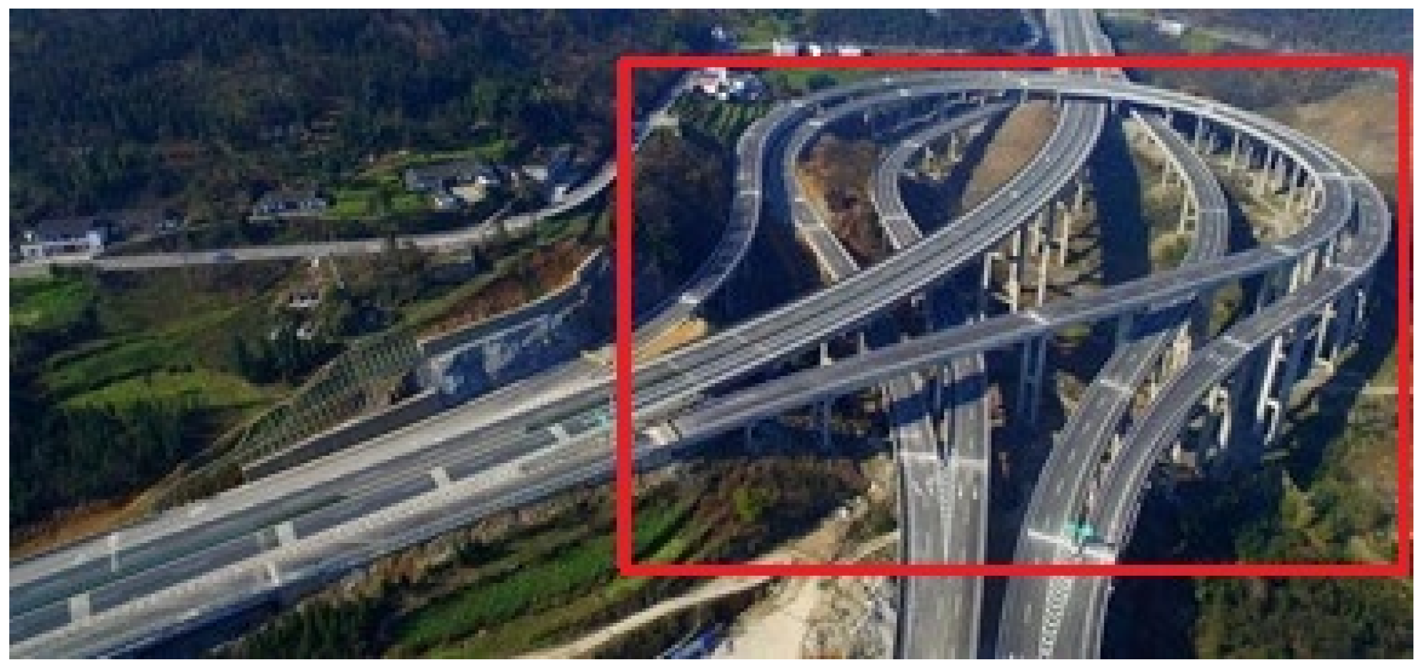
Search for changes in grayscale values along the image’s width or height direction, and record the positions of pixels where the grayscale values suddenly increase or decrease. Connect these points to form an information-rich target area, and then crop the image to this area as the ROI, as shown in Figure 3. The ROI obtained by this algorithm effectively eliminates the effects of noise, rotation, translation, etc. Experiments have shown that the ROI obtained by this method is more conducive to subsequent feature extraction.

Figure 3.
Selecting areas of interest. The area of interest in the traffic map is indicated by a red box.
The ROI area segmented by this algorithm is large and almost completely covers the turning points on the traffic map, which improves the accuracy of subsequent feature extraction and feature matching.
3.2. Extract Key Turning Point Characteristics Within ROI
Image features are a reflection of the discontinuity of local characteristics of the image, which marks the end of one area and the beginning of another area. The discontinuities in the local characteristics of the image can be easily detected using first- and second-order derivative methods. Feature detection can be achieved by convolving the image with spatial differential operators, or using the discrete Z-transform for convolution. Here, a given digital matrix is used as a template to perform discrete convolution on the image. The method is as follows:
Implement feature extraction on the target image. Assume that the operators used are two 3 × 3 operators. Perform discrete convolution on the image to obtain the horizontal () and vertical () gradient values, respectively. If the combined gradient magnitude exceeds a certain threshold , the point is considered a feature point and is marked. The method for extracting objects from images is as follows:
3.2.1. Convolution Operation Between the Extraction Algorithm and the Target
A and B are templates, and I is an image, Then:
3.2.2. Gradient and Direction
Calculate the gradient value of the image; that is, the horizontal and vertical feature values of each pixel of the image are calculated using the following formula to calculate the size of the point feature:
To calculate the approximate gradient magnitude of an image, a non-square root approximation is usually used to improve efficiency:
The gradient direction can then be calculated using the following formula:
Given a threshold value , if , the point is considered an edge point, and its feature information is stored. Then, the pixel values in flat areas are masked, and only the stored feature pixels are displayed. In this way, the feature edges are extracted.
Next, smooth the features: Let the original image be . Use a low-pass filter H to smooth in the spatial domain, and the output image is :
After filtering, an image with relatively complete target features can be obtained, and then an appropriate threshold h is selected to binarize . The processed image is :
Based on this image feature extraction algorithm, the results of the traffic map feature extraction are shown in Figure 4.
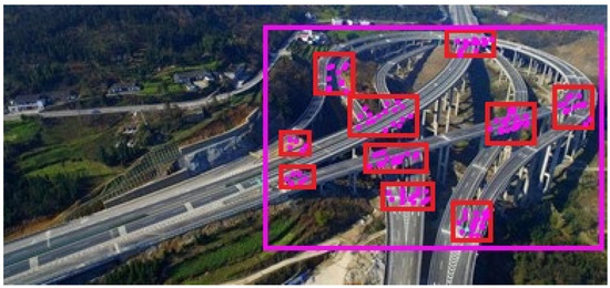
Figure 4.
Feature extraction within the area of interest. The purple box represents the area of interest, the red box represents the turning point area of interest, and the purple dots represent the key turning points of the extracted route.
As can be seen from Figure 4, on the given image, the feature extraction algorithm can completely outline the turning point features, eliminate background effects, reduce noise, and contain almost all the information of the traffic map. In experiments, it was found that its extraction effect is better than that of other existing algorithms.
4. Interpolating Between Turning Points
After extracting the key turning points above, and according to mechanical analysis theory, the car can drive along a continuous curve with a certain arc radius, allowing it to move smoothly, effectively avoid obstacles and ensure safety. Therefore, it is necessary to consider two key aspects of path optimization. We add virtual points between turning points. Here, the cubic spline interpolation method is given as follows:
Let be the cubic interpolation function of the position nodes in the horizontal direction X and vertical direction Y. Here, X refers to the set of the abscissae of the position nodes, and Y refers to the set of ordinates of the position nodes. Then, , , and . Let us assume that the second derivative at each node is .
Since in each subinterval is a polynomial of at most three degrees, its second-order derivative is a linear function in each subinterval, given by
while . If we integrate twice and apply the node conditions,
Then, we can obtain the expression of the cubic interpolation function on the subinterval as follows:
Here, and are the second derivatives at the endpoints and of the subinterval , respectively. It follows that once the second derivatives at each node are determined, the cubic function on each subinterval is also determined.
Using the above method with Equation (8), by pairing data points, Equation (8) can be extended into a higher-dimensional function. Figure 5 shows the relationship between the function obtained with this fitting method and the actual measured data.
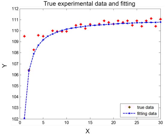
Figure 5.
Relationship between fitted function and measured data.
As shown in Figure 5, the cubic interpolation function closely fits all the actual measured data.
5. Define Valuation Function
5.1. Valuation Function
According to queuing theory, the occurrence of congestion can be modeled as a Poisson process, and the time intervals between vehicles on the road follow an exponential distribution. Therefore, if the traffic flow density on the road is , the probability of k congestion arrivals in time period is
Here, represents the number of congestion events within the time interval .
Let be the congestion intensity of the i-th road with the probability distribution function , where . The congestion intensities at different intervals are independent and identically distributed, each following a Poisson distribution. represents the i-fold reconvolution of G. In addition, it is assumed that the loss function of fuel consumption, vehicle wear, time, etc., caused by congestion on the traffic road is , and the interval time is T. When the congestion level on the road reaches the threshold h, the traffic management’s processing capacity becomes insufficient or fails. Then, before the time T, the congestion loss rate function is
Since traffic congestion requires a cost per unit loss c to recover, the total recovery cost is :
The fifth part of the global search for the optimal path method ensures that Equation (11) is minimized.
In addition, if there are m roads with n self-driving cars on them, then the evaluation function can be defined as follows.
Let there be m roads labeled as . If the roads that can be selected when the i-th vehicle enters at a given time are , then the road smoothness probability is , which is a function of the selected roads and can be written as . Therefore, how should vehicles choose these roads to minimize congestion on all roads, that is, to maximize Equation (12), where
Equation (12) is the evaluation function of this problem.
According to Equations (12) and (13) obtained from the above analysis, it can be seen that the meaning and form of the evaluation function are different according to the needs of different situations. It is also possible to use the shortest path and the minimum number of intersections as the optimization objectives and the vehicle load as the constraint to obtain an evaluation function. Based on the above situation analysis, the piecewise function in the following form can be defined as the evaluation function of path planning.
Here, is the estimation function, is the demand situation, is the threshold or condition, 1 is the first strategy, and 2 is the second strategy. If the graph is an even-degree vertex graph, strategy 1 is adopted. Driving along any road on the traffic map can satisfy customer needs at minimal cost. If the even-numbered vertex graph is not satisfied, strategy 2 is adopted to recognize the traffic network graph. An even-degree vertex graph can be constructed by adding edges between two odd-degree vertices. At this time, driving along any road on the traffic map can also satisfy the needs of customers on the traffic line, and the cost is minimal. This method is the global optimal path planning method in Section 6 of the next chapter.
5.2. Simulation of the Valuation Function
Here, the evaluation function Equation (11) is simulated. Assuming , we can know that
From Equation (11), we obtain
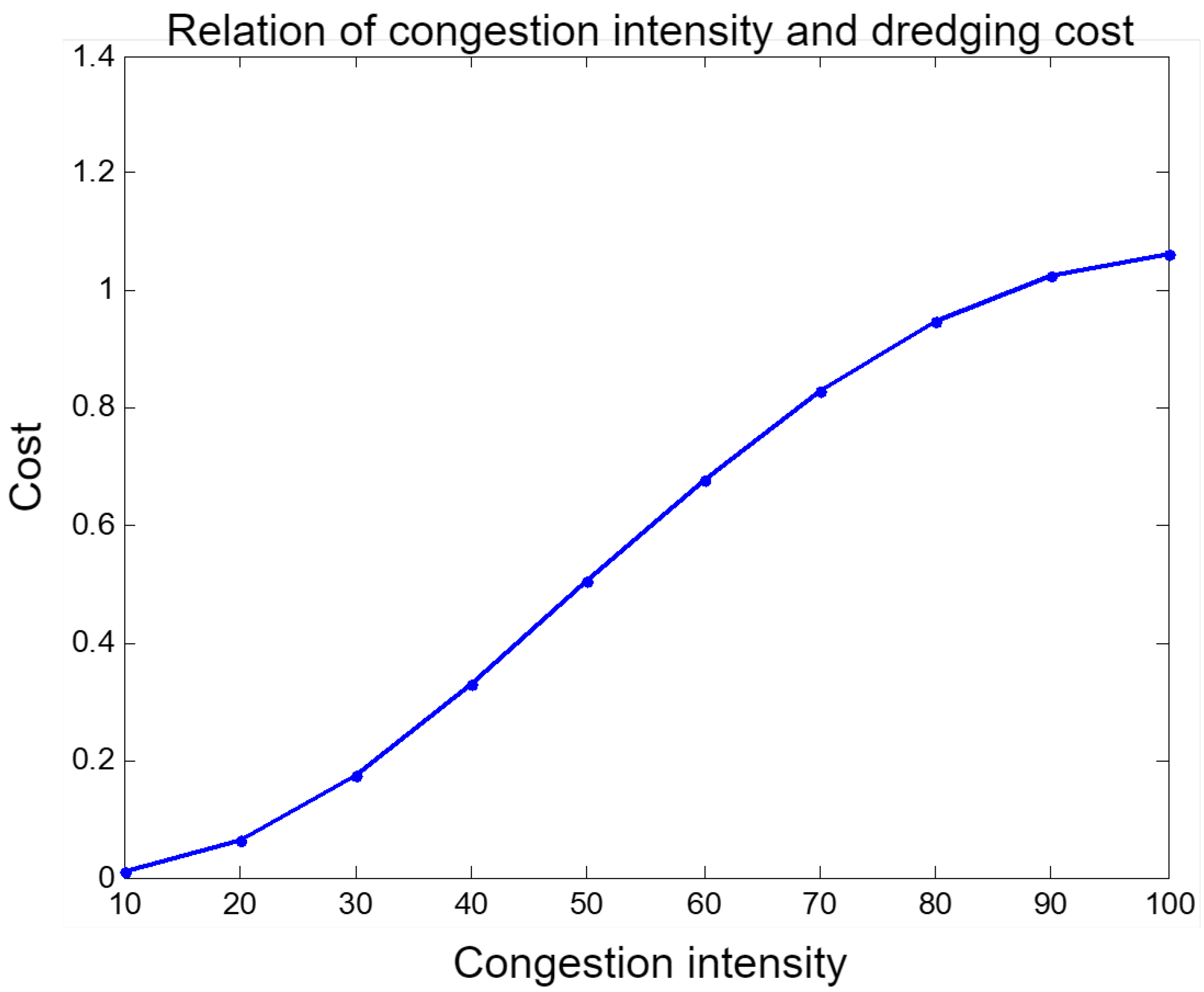
Assume that , or 0.2, and that maintenance cost C = 6.2. Since the road congestion threshold can be obtained by measurement, it is assumed that is known. When the congestion threshold is 100 vehicles per unit area, the trend in the toll cost function with respect to the congestion level is shown in Figure 6. It can be seen from Figure 6 that as the congestion intensity increases, the clearing cost increases. When the congestion reaches a critical value, the clearing cost tends to stabilize.
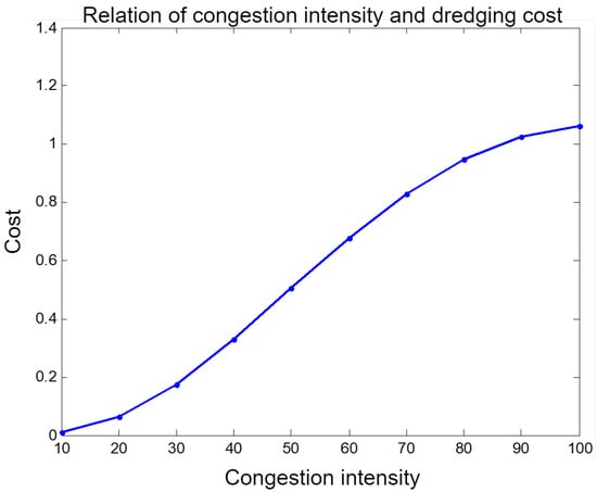
Figure 6.
The relationship between congestion intensity and dredging and maintenance costs.
6. Global Optimal Path Search Method
6.1. Euler Search Method
Now let us consider finding the minimum weight tour in a weighted connected graph, i.e., the optimal tour. The road network on which driverless buses transport passengers can be modeled as a weighted connected graph. It must start from the starting station, traverse each required road at least once, and then return to the starting station; thus, the path is a closed tour.
If the traffic graph G is a Euler graph, then any Euler tour is the optimal tour. Currently, the algorithm for finding the optimal tour is as follows:
(1) Take any vertex and let .
(2) If trace has been determined, select such that
➀ is related to .
➁ Unless there is no alternative, choose such that it is not a bridge in subgraph .
(3) If step (2) cannot be continued, stop.
If G is not a Euler graph, then its optimal tour obviously requires the repeated traversal of some paths, so that it is possible to traverse each path at least once and eventually return to the starting point. It is easy to see that in any optimal tour of G, each edge is repeated at most once. In the weighted connected graph G, finding a minimum weight tour, i.e., the method for finding the optimal tour, is as follows:
(1) Add duplicate edges to G to create a Eulerian supergraph , minimizing the total weight of the added edges . In other words, the required is a Eulerian supergraph of G with the minimum total added edge weight.
(2) Find its Euler tour in .
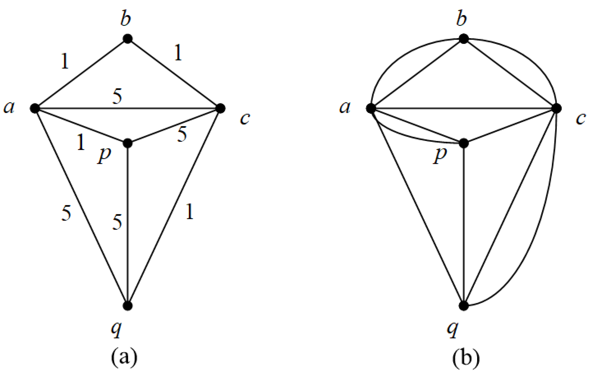
The following is the simplest case, i.e., if there are exactly two odd-degree vertices p and q in the weighted graph G, it is proved that can be obtained by adding repeated edges along the shortest -path P in G, as shown in Figure 7. The numbers in Figure 7 represent the cost of each edge. In G, only p and q are ; its shortest -path is ; the total weight of the added repeated edges is 4.
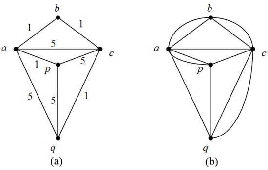
Figure 7.
(a) is the weighted graph G and (b) is the optimal Euler generated parent graph .
Proof.
It is easy to see that only p and q are odd-degree vertices in . Since the number of odd-degree vertices is even, the two odd-degree vertices must be in the same component of . Let be one of the -paths; then, we have
However, the graph obtained by adding duplicate edges along the shortest -path P in G is also a Eulerian supergraph of G, so it is the desired .
Here, and represent the number of vertices and edges of graph G, respectively, represents the weight of graph G, and represents all edges of graph G. □
In fact, when looking for other paths, first check whether each vertex of the traffic graph composed of key points on the map in the area is an even-degree vertex. If so, starting from any point yields the optimal path; if not, you need to calculate the shortest paths between all pairs of odd-degree vertices along the traffic graph and select the minimum among these calculated shortest paths. At this point, the corresponding two odd-degree vertices can be denoted as A and B, and a duplicate path is added along the path from A to B. Ensure that the other vertices between points A and B are also even-degree vertices. Based on the definition of the cost function in Part 4 and the global optimal path planning of the path, this search algorithm ensures that each traffic line can be traversed at the lowest cost.
6.2. Reverse Search Method
For evaluation Function (12), from the Euler diagram of the figure, the global optimal path search method is as follows: introduce a function that represents the maximum smoothness rate that can be obtained when the number of roads chosen by the first to K-th vehicles ; here, . Obviously, represents the maximum smoothness obtained by all n vehicles when they choose road number .
For evaluation Function (12), based on the Euler diagram in the figure, the global optimal path search method involves introducing a function that represents the maximum smoothness rate that can be obtained when the cumulative number of times road j has been chosen by the first to the K-th vehicles is , where and . Obviously, this represents the maximum smoothness obtained when all n vehicles have chosen a road.
Now let us derive the relation that should satisfy. It is known that the cumulative number of times road j has been chosen by the first K vehicles is . If the number of times road j is chosen by the K-th vehicle is , then the cumulative number of times road j has been chosen by the previous vehicles is . Considering the choices of the K vehicles as a K-step decision process, represents the optimal index value of the K-step decision; that is, it represents the smoothness probability value of the K-th step when the number of times road j is chosen is ; represents the optimal value of the remaining decision steps. According to the principle of optimality, we have
This shows that if the optimal choices of the first to the K-th vehicles for road j are , then the optimal allocation of among the first vehicles is , where and .
This type of optimal planning has two characteristics: first, it is computed backward from the last stage; second, it transforms an n-stage decision problem into n single-stage decision problems, i.e., it transforms a complex problem into multiple simpler problems to solve.
7. Experiment
In order to compare the advantages of the proposed global path optimization algorithm with existing path optimization algorithms, this study conducted experiments on a dataset. The dataset sources were divided into two parts: (1) data collected by the developed verification platform; (2) data from a road section under the jurisdiction of a transportation bureau. Based on this, an evaluation method was designed.
7.1. Verification Platform Construction
The platform used to verify the effectiveness of the algorithm is a self-developed mobile robot, as shown in Figure 8.
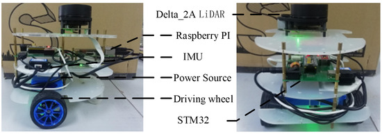
Figure 8.
Physical image of verification platform.
7.2. Datasets
The steps to create the path databases and test sample databases for the three traffic types used in the experiment—sparse traffic, medium-density traffic, and complex traffic—are as follows:
➀ Randomly select 200 traffic routes under different environments from the collected databases of the three traffic types. For each route, randomly select 2 traffic maps out of 10 available traffic maps, resulting in a total of 400 traffic maps.
➁ From each route’s 2 traffic maps, randomly select 1, totaling 200, to form the experimental traffic map database; the remaining 200 traffic maps form the test sample database.
➂ Apply the above global optimal search method to perform optimal path planning on the 200 traffic maps in the experimental traffic map database, obtaining 200 planning templates, each containing a labeled map. Store the planned labeled maps in the collected traffic library as training samples.
7.3. Problem Definition
In this study, the problem of global optimal path planning for driverless cars is defined as follows: the optimal global path of the vehicle is planned based on the traffic map collected by the integrated camera, and the globally optimized path map is used as the output. The input is the traffic map , and the output is the optimal global path planning map , where t represents time (Figure 9).

Figure 9.
Traffic map.
7.4. Evaluation Methodology
A path planning and optimization path counting program was developed. Assume that a total of optimization path experiments were performed in the i-th time period, and times were counted as optimal paths by the counting program. The experiment was repeated times. Then, the accuracy of the i-th experimental optimization path is defined as
The total average accuracy , repeated times, is
After many experiments, we found that when the experiment was repeated approximately 50 times, the results tended to stabilize, so we finally chose to repeat the experiment 50 times as the standard.
7.5. Evaluation of the Correctness of Optimal Path Planning
The basic evaluation steps are as follows:
P1. Use the global optimal search method to perform optimal path planning on the traffic maps in the test sample library to obtain the planned maps, and then match the obtained planned maps with the samples in the traffic library.
P2. Compare the traffic map to be tested with all optimal traffic maps in the training sample gallery, perform 100 random selection and matching tests, and take the traffic map corresponding to the most similar one as the test result.
P3. Test each traffic map in the test sample database 100 times according to steps P1∼P2, record the number of correct and incorrect planning results, and calculate the correct planning rate.
7.6. Quantitative Results
For each traffic map, 20 repeated experiments were performed according to steps P1 to P3 in the simulation. Each experiment used a different number of samples and was compared with the current optimal planning methods [18,25]. After 100 simulations, the average optimal planning accuracy rates were 96.71%, 87.85%, and 79.69%, respectively. The simulation results are shown in Figure 10 and Table 2.
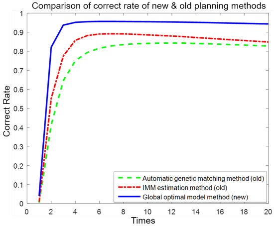
Figure 10.
Comparison of accuracy between the proposed method and existing optimal path planning methods.
Table 2.
Comprehensive comparison of proposed and existing optimal planning algorithms.
As shown in Figure 10, in the experiment, at the beginning, the environment was unknown, the accuracy was low, and the ability of several optimization methods to block noise was weak. As the number of experiments increased, the average accuracy continued to increase, which also means that it has a better ability to clear congestion. When the number of experiments reached a certain number, the curve did not change much when the number of experiments was increased. The three methods gradually stabilized because they all had memory functions. The ability to block noise increased after repeating the path many times. If the experiment continued, they were basically in a stable state.
As shown in Figure 10, at the beginning of the experiment, the environment was unknown, the accuracy was low, and the ability of several optimization methods to filter noise was weak. As the number of experiments increased, the average accuracy continued to rise, which also indicates a better ability to alleviate congestion. When the number of experiments reached a certain point, the curve did not change significantly with further increases in the number of experiments. The three methods gradually stabilized because they all have memory functions. The ability to filter noise improved after repeating the path many times. If the experiment continued, they would basically remain in a stable state.
As shown in Table 2, the accuracy of the global optimal path planning method proposed in this paper was compared with existing path optimal planning methods [18,25]. The experimental results show that the average accuracy of the global optimal path planning algorithm proposed in this paper is 96.71%, the average accuracy of the IMM estimation method [25] is 87.85%, and that of the automatic genetic matching method [18] is 79.69%. In addition, the search speed of the algorithm in this paper is 2.78 ms, while that of the IMM estimation method is 3.82 ms, and the automatic genetic matching method is 4.08 ms. Compared with existing planning algorithms, the proposed method has a higher correct planning rate, a shorter optimization time, and a stronger anti-noise ability, making it suitable for sparse, medium-density, and dense complex environments.
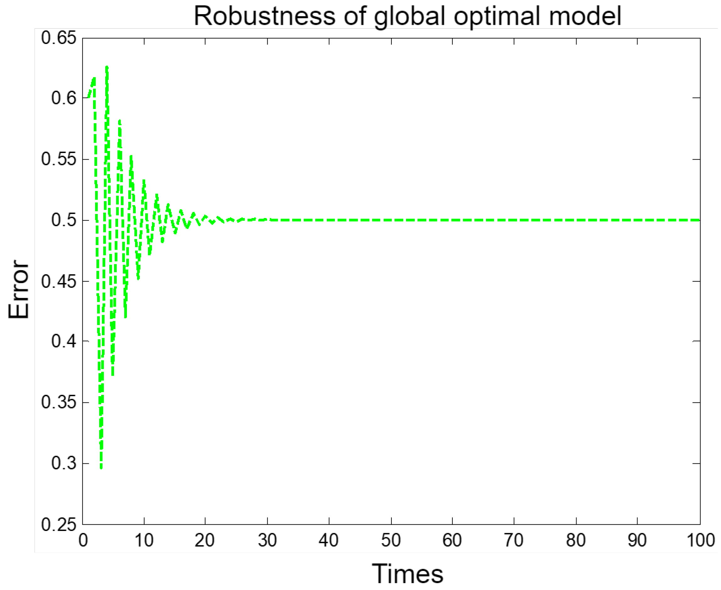
Finally, to verify that the established global optimal path planning model was stable and robust, a stability experiment was conducted. The results show that the error gradually decreases as the number of experiments increases, tending toward stability and convergence, indicating that the established global optimal path planning model has stable performance and strong anti-noise ability. Here, the error is a relative difference, that is, the ratio of the absolute value of the difference between the estimated value of the model and the true value to the true value, as shown in Figure 11.

Figure 11.
Robustness of the global optimal path planning model.
As can be seen from Figure 11, the vibration amplitude of the optimal planning model is large at the beginning, and then gradually converges to a stable value as the number of experiments increases. This shows that the established global optimal path planning model is truly stable and convergent.
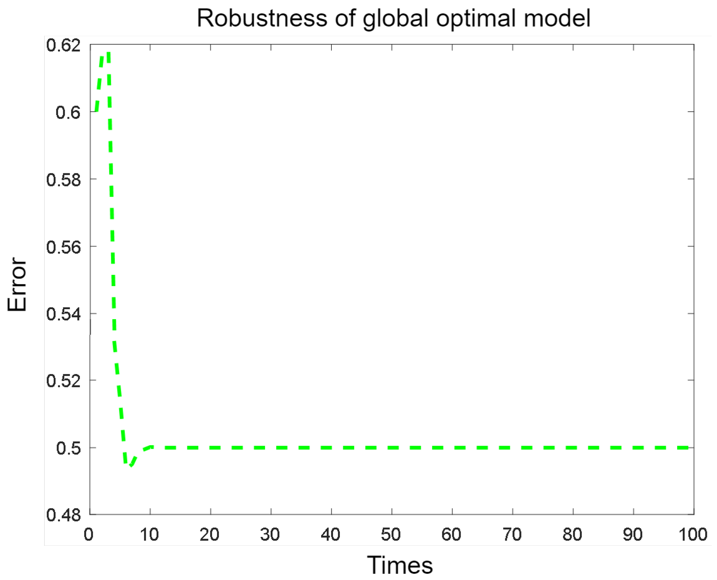
After adding a noise reduction smoothing filter in front of the physical platform device in Figure 8, the oscillation amplitude of the previous planning model is improved, and its vibration amplitude is significantly reduced, as shown in Figure 12.
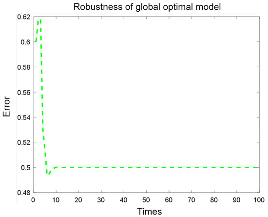
Figure 12.
The vibration amplitude of the optimal planning model is reduced.
7.7. Qualitative Results
As show in Figure 13, the map area increases, the complexity also increases. The upper half of the map contains more concave obstacles, while the obstacles in the lower half are randomly distributed. The proposed algorithm can navigate through concave or randomly distributed obstacles with fewer turning points, and the quality of the generated path is significantly improved compared to traditional algorithms.
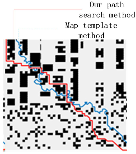
Figure 13.
The proposed algorithm plans the path for complex traffic conditions.
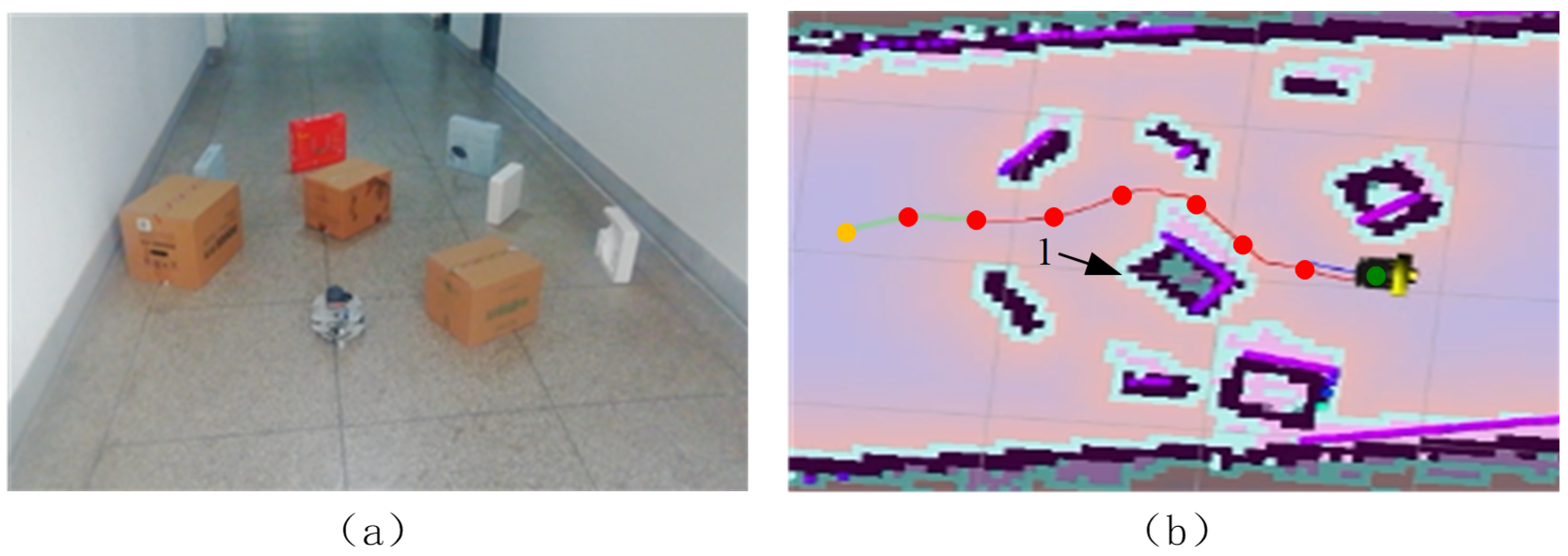
A relatively complex test environment is designed for the algorithm proposed in this paper. The actual scene is shown in Figure 14a.
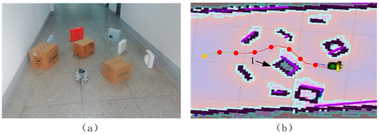
Figure 14.
The generated path is realized based on the path search method proposed in this paper. (a) is the experimental scene, and (b) is the generated car path in this scene.
The path generated by the unmanned driving path search method proposed in this paper is shown in Figure 14b, where the starting point and the end point are marked in green and yellow, respectively, and the generated path is marked in red. The path shown in the figure represents the movement path of the robot chassis center. When avoiding obstacle No.1, the expansion layer adjacent to the obstacle is used. Due to the presence of an expansion layer, the robot could traverse this area smoothly.
In Figure 14b, the generated path first moves forward for a distance and then turns right to avoid the obstacle on the left. Although the path generated by the proposed algorithm is close to the obstacle, due to the presence of the expansion layer, the robot can still safely avoid obstacle No.1. At this point, the mobile robot is surrounded by obstacles and is prone to collision. Therefore, it needs to move at a lower speed. After turning right, it moves to the left. At this point, there are obstacles on both sides of the robot. The generated path maintains a safe distance from the obstacles on both sides, which improves the safety of the robot’s passage. The subsequent path gradually moves away from the obstacles and finally reaches the end position.
In summary, in an actual environment where obstacles appear randomly in size, orientation, and spacing, the path generated by the path search method proposed in this paper can plan a path that keeps as far away from obstacles as possible while minimizing path length, thereby improving the travel efficiency and safety of the mobile robot.
8. Conclusions
In order to ensure that autonomous traffic can continue to provide reliable services and reduce the safety hazards caused by improper path planning, this paper proposes a global optimal path planning model. By extracting the key turning points of the path and performing cubic interpolation between them, an evaluation function for driving route change decisions is provided, and the Euler graph path search algorithm is proposed. The experimental results verify the feasibility and effectiveness of the model for autonomous vehicles. The comparison shows that the optimal path planning method proposed in this paper is superior to existing optimal path planning algorithms in terms of path selection accuracy, path determination speed, and robustness against external interference.
The method proposed in this paper is deployed in an autonomous traffic section in a certain area. In an environment where there is an obstacle in each path, the planned optimal path speed reaches 80 km/h; however, under strong light and backlight conditions, the performance is reduced and can only reach 60 km/h, which is a limitation of the current research. Future research can target this weakness and further improve the robustness of the algorithm in complex lighting environments, possibly by improving the perception system or optimizing the algorithm’s adaptability to lighting changes. In addition, the practicality and applicability of the model should be expanded to enable it to cope with more complex real-world scenarios and diverse obstacle distributions.
Author Contributions
Conceptualization, Q.W. and F.W.; methodology, S.S. and Q.W.; software, F.W. and S.S.; validation, Q.W., S.S. and F.W.; formal analysis, Q.W.; investigation, Q.W.; resources, Q.W.; data curation, S.S.; writing—original draft, Q.W., F.W. and S.S.; writing—review and editing, Q.W., F.W. and S.S.; visualization, Q.W.; supervision, Q.W.; project administration, Q.W.; funding acquisition, Q.W. All authors have read and agreed to the published version of the manuscript.
Funding
This work is supported by Key Science and Technology Program of Henan Province (No. 222102210084) and the Fourth Intelligent Compilation Zhengzhou 1125 Science and Technology Innovation Talents (192101059006).
Data Availability Statement
The data required to reproduce these findings cannot be shared at this time as the data also form part of an ongoing study. They can be requested from the author by e-mail (qewu@sspu.edu.cn) in the future.
Conflicts of Interest
The authors declare no conflicts of interest.
References
- Wu, W.; Liu, Y.; Wei, L.; Wu, G.; Ma, W. A novel autonomous vehicle trajectory planning and control model for connected-and-autonomous intersections. Acta Autom. Sin. 2020, 46, 1971–1985. [Google Scholar]
- Fan, H.; Liu, P.; Liu, H.; Hou, D. The multi-depot vehicle routing problem with simultaneous deterministic delivery and stochastic pickup based on joint distribution. Acta Autom. Sin. 2021, 47, 1646–1660. [Google Scholar]
- Li, S.; Zheng, H.; Yang, C.; Wu, C.; Wang, H. Research on Hybrid Path Planning Algorithm Based on A* and DWA Algorithm. J. Jilin Univ. (Inf. Sci. Ed.) 2022, 40, 132–141. [Google Scholar]
- Li, Y.; Tong, C. Research on optimal path planning for vehicle navigation based on multi-objectives. Sci. Technol. Innov. 2021, 26, 27–28. [Google Scholar]
- Li, X.; Xiong, H.; Tao, Y.; Li, G. Global optimal path planning for mobile robots based on improved A* algorithm. High Technol. Lett. 2021, 31, 306–314. [Google Scholar]
- Liu, J.; Ji, H.; Li, Y. Robot Path Planning Based on Improved Bat Algorithm and Cubic Spline Interpolation. Acta Autom. Sin. 2021, 47, 1710–1719. [Google Scholar]
- Hu, Z.; Yang, Z.; Liu, X.; Zhang, W.; Luo, R. Radar-based maritime path planning with static obstacles in a Frenet frame. Sci. Sin. Technol. 2021, 51, 1401–1409. [Google Scholar] [CrossRef]
- Li, J.; Liu, S.; Qian, Y. Optimal Path Planning of UAV Fleet Based on Terminal Vision Navigation. Value Eng. 2021, 40, 3. [Google Scholar]
- Zhang, X.; Xie, Z.; Wu, H. Obstacle Avoidance Path Planning Method for Power Grid Inspection Robot Based on Time Grid Method and Optimal Search. Mach. Electron. 2021, 39, 71–75. [Google Scholar]
- Xing, Q.; Chen, Z.; Leng, Z.; Lu, Y.; Liu, Y. Route Planning and Charging Navigation Strategy for Electric Vehicles Based on Real-time Traffic Information. Proc. CSEE 2020, 40, 534–550. [Google Scholar]
- Xiao, Y. Optimal Patrolling Path Planning Method and Application Based on Linear Temporal Logic. Master’s Thesis, Zhejiang University of Technology, Hangzhou, China, 2014. [Google Scholar]
- Zhou, B.; Tang, L.; Liu, S. Design of Path Planning for Underground Vehicle Based on Genetic Algorithm. Coal Mine Mach. 2022, 43, 23–26. [Google Scholar]
- Gao, Z.; Dai, X.; Zheng, Z. Optimal Energy Consumption Trajectory Planning for Mobile Robot Based on Motion Control and Frequency Domain Analysis. Acta Autom. Sin. 2020, 46, 934–945. [Google Scholar]
- Fu, Z.; Chow, J.Y. The pickup and delivery problem with synchronized en-route transfers for microtransit planning. Transp. Res. Part Logist. Transp. Rev. 2022, 157, 102562. [Google Scholar] [CrossRef]
- Li, K.; Rao, X.; Pang, X.; Chen, L.; Fan, S. Route search and planning: A survey. Big Data Res. 2021, 26, 100246. [Google Scholar] [CrossRef]
- Nahum, O.E.; Wachtel, G.; Hadas, Y. Planning tourists evacuation routes with minimal navigation errors. Transp. Res. Procedia 2020, 47, 235–242. [Google Scholar] [CrossRef]
- Yin, J.L.; Chen, B.H.; Peng, Y.T.; Hwang, H. Automatic intermediate generation with deep reinforcement learning for robust two-exposure image fusion. IEEE Trans. Neural Netw. Learn. Syst. 2021, 33, 7853–7862. [Google Scholar] [CrossRef]
- Avola, D.; Cinque, L.; Fagioli, A.; Foresti, G.L.; Pannone, D.; Piciarelli, C. Automatic estimation of optimal UAV flight parameters for real-time wide areas monitoring. Multimed. Tools Appl. 2021, 80, 25009–25031. [Google Scholar] [CrossRef]
- Han, C.; Li, B. Mobile robot path planning based on improved A* algorithm. In Proceedings of the 2023 IEEE 11th Joint International Information Technology and Artificial Intelligence Conference (ITAIC), Chongqing, China, 8–10 December 2023; IEEE: Piscataway, NJ, USA, 2023; Volume 11, pp. 672–676. [Google Scholar]
- Babu, A.; Kavitha, T.; de Prado, R.P.; Parameshachari, B.D.; Woźniak, M. HOPAV: Hybrid optimization-oriented path planning for non-connected and connected automated vehicles. IET Control Theory Appl. 2023, 17, 1919–1929. [Google Scholar] [CrossRef]
- Shi, K.; Wu, Z.; Jiang, B.; Karimi, H.R. Dynamic path planning of mobile robot based on improved simulated annealing algorithm. J. Frankl. Inst. 2023, 360, 4378–4398. [Google Scholar] [CrossRef]
- Lin, S.; Liu, A.; Wang, J.; Kong, X. An intelligence-based hybrid PSO-SA for mobile robot path planning in warehouse. J. Comput. Sci. 2023, 67, 101938. [Google Scholar] [CrossRef]
- Ding, J.; Zhou, Y.; Huang, X.; Song, K.; Lu, S.; Wang, L. An improved RRT* algorithm for robot path planning based on path expansion heuristic sampling. J. Comput. Sci. 2023, 67, 101937. [Google Scholar] [CrossRef]
- Caponetto, R.; Fortuna, L.; Graziani, S.; Xibilia, M. Genetic algorithms and applications in system engineering: A survey. Trans. Inst. Meas. Control 1993, 15, 143–156. [Google Scholar] [CrossRef]
- Blom, H.A.; Bar-Shalom, Y. The interacting multiple model algorithm for systems with Markovian switching coefficients. IEEE Trans. Autom. Control. 1988, 33, 780–783. [Google Scholar] [CrossRef]


Disclaimer/Publisher’s Note: The statements, opinions and data contained in all publications are solely those of the individual author(s) and contributor(s) and not of MDPI and/or the editor(s). MDPI and/or the editor(s) disclaim responsibility for any injury to people or property resulting from any ideas, methods, instructions or products referred to in the content. |
© 2024 by the authors. Licensee MDPI, Basel, Switzerland. This article is an open access article distributed under the terms and conditions of the Creative Commons Attribution (CC BY) license (https://creativecommons.org/licenses/by/4.0/).