SOAMC: A Semi-Supervised Open-Set Recognition Algorithm for Automatic Modulation Classification

Abstract

Traditional automatic modulation classification methods operate under the closed-set assumption, which proves to be impractical in real-world scenarios due to the diverse nature of wireless technologies and the dynamic characteristics of wireless propagation environments. Open-set environments introduce substantial technical challenges, particularly in terms of detection effectiveness and computational complexity. To address the limitations of modulation classification and recognition in open-set scenarios, this paper proposes a semi-supervised open-set recognition approach, termed SOAMC (Semi-Supervised Open-Set Automatic Modulation Classification). The primary objective of SOAMC is to accurately classify unknown modulation types, even when only a limited subset of samples is manually labeled. The proposed method consists of three key stages: (1) A signal recognition pre-training model is constructed using data augmentation and adaptive techniques to enhance robustness. (2) Feature extraction and embedding are performed via a specialized extraction network. (3) Label propagation is executed using a graph convolutional neural network (GCN) to efficiently annotate the unlabeled signal samples. Experimental results demonstrate that SOAMC significantly improves classification accuracy, particularly in challenging scenarios with limited amounts of labeled data and high signal similarity. These findings are critical for the practical identification of complex and diverse modulation signals in real-world wireless communication systems.

1. Introduction

In modern communication systems, different modulation schemes directly impact data transmission performance and spectral efficiency. As such, the accurate identification of modulation modes plays a critical role in signal processing, resource allocation, and overall system optimization. Automatic modulation classification (AMC) [1,2,3] represents a significant technological advancement that enables the automatic detection of the modulation scheme used in a received signal. Widely applied in the field of communications, AMC technology is instrumental in optimizing system performance, efficiently allocating resources, and effectively managing the communication spectrum by precisely identifying modulation schemes.

Despite its advancements, the field of AMC continues to encounter significant challenges, including signal noise, multipath fading, and frequency offset, all of which contribute to signal degradation. Furthermore, the increasing diversity and complexity of modulation schemes intensify the difficulty of the classification task. As AMC is inherently a pattern recognition problem, the integration of artificial intelligence (AI) technologies, such as intelligent signal processing [4,5,6], has emerged as a promising solution in electromagnetic signal processing. With ongoing technological advancements, AI has demonstrated substantial potential in improving pattern recognition. In particular, deep learning [7,8], renowned for its ability to automatically extract complex features and enhance recognition accuracy, has been extensively adopted in this field.

In the field of deep learning research on signal modulation classification, the collection of a substantial volume of electromagnetic sample signals is crucial for supervised training. However, this process typically requires considerable human and material resources. The acquisition of radio frequency (RF) signals from the environment involves the use of various spectrum acquisition devices and signal processing techniques to generate visual representations of signals, such as afterglow plots, waterfall plots, and spectrum maps. Signal analysis in this context demands experts to carefully examine the time-frequency characteristics of the signals in order to accurately identify the target signal. This technology necessitates a high level of expertise and technical proficiency from operators. Nevertheless, as the volume of radio signals increases or the monitoring period extends, the efficiency and accuracy of manual analysis significantly decline. To overcome these challenges, semi-supervised learning [9,10] offers a promising solution in modulation signal recognition by reducing the dependence on labeled samples. Through the use of semi-supervised learning algorithms, a large volume of unlabeled modulation signal samples can be leveraged for model training, even when only a limited number of labeled samples are available. This approach significantly reduces the need for labeled data and enhances both the efficiency and accuracy of modulation signal recognition.

With the rapid advancement of communication technology, the need for effective communication signal recognition has become increasingly urgent. In the domain of communication signal classification and recognition, deep learning has achieved significant progress. However, existing methods typically assume that test samples belong to the known categories present in the training set, an assumption that often does not hold true in practical applications. As a result, the challenge of open-set recognition (OSR) has gained considerable attention. The objective of OSR is to develop algorithms capable of handling unknown category samples, thereby enhancing the robustness and generalization ability of machine learning systems. Compared to traditional closed-set recognition, OSR presents greater challenges. In an open-set environment, it is impossible to obtain training data that encompasses all possible categories in advance, making it difficult to distinguish unknown category samples from known categories. To address this issue, researchers have proposed a range of innovative methods and techniques, including anomaly detection algorithms, generative models, and metric learning approaches. These methods aim to establish robust decision boundaries that can effectively differentiate between unknown and known category samples.

In this paper, to accurately detect unknown categories and perform the fine-grained recognition of multiple unknown categories in AMC, we propose a semi-supervised open-set recognition algorithm, called SOAMC. We first use labeled signals and a large number of unlabeled signals to train a pre-trained model. To improve the robustness of the model, we applied various data augmentation methods, including flipping, rotation, noise addition, and CutMix. Meanwhile, we designed a self-adaptive thresholding (SAT) adjustment method to ensure the quality of the pseudo-labels. The SAT does not require manual threshold-setting; instead, it automatically adjusts the threshold by monitoring the model’s training process. This allows it to adapt to different data distributions and learning difficulties at various training stages, thereby making better use of the unlabeled samples. We then propose an open-set feature embedding strategy by treating all newly emerging categories as incremental categories and fine-tune the pre-trained model using these unlabeled signals, which can make the classifier possess some supervised information of the newly emerging categories’ classes. Then, in the testing stage, a few labeled samples of increment classes and unlabeled samples are connected based on the extracted features by the new classifier to obtain an undirected distance-based similarity graph, where Euclidean distance is used to measure the similarity between two nodes. Our proposed method predicts the labels of unlabeled samples through the label propagation algorithm, which propagates the label information from the labeled nodes to the unlabeled nodes in the graph.

In summary, we have made the following three main contributions:

•

We propose a semi-supervised open-set modulation recognition algorithm called SOAMC, which performs label propagation on a large number of unlabeled samples. This approach effectively addresses the challenge of automatic modulation classification and recognition in open environments, relying only on a small number of labeled samples.

•

We design an adaptive enhancement module that leverages data augmentation and adaptive modulation techniques to significantly enhance the robustness of the pre-trained model. Experimental results demonstrate that this module effectively improves the model’s recognition accuracy, even when only a small number of labeled samples are available.

•

We propose an open-set feature embedding strategy that effectively utilizes a minimal number of labeled samples to achieve accurate classification in open-set modulation recognition. The effectiveness of the proposed algorithm is validated through simulation experiments.

The following introduces the general content of each section of this article. In Section 2, related works are elaborated upon. In Section 3, we introduce SOAMC, a semi-supervised open-set modulation recognition algorithm, and describe the proposed method in detail. The simulation results are presented in Section 4, while Section 5 provides a summary of the conclusions.

2. Related Works

2.1. Semi-Supervised Learning

Semi-supervised learning (SSL) is a machine learning approach that lies between the supervised and unsupervised learning paradigms. It leverages a small set of labeled data alongside a large amount of unlabeled data for pattern recognition [11,12]. The primary goal of SSL is to overcome the limitations of supervised and unsupervised methods by enabling the model to autonomously leverage unlabeled samples and improve performance without external intervention.

A prominent research focus in semi-supervised learning is pseudo-labeling [13]. In [14], Zou et al. introduced the Confidence-Regularized Self-Training (CRST) method, which treats pseudo-labels as continuous hidden variables and iteratively refines them through optimization. The approach employs two regularization techniques. The first, label regularization, enhances the entropy of pseudo-labels during the labeling process, similar to label smoothing. The second, model regularization (MR), increases the entropy of network output probabilities during network retraining. The experimental results presented by the authors confirm the effectiveness of confidence regularization. Specifically, when the pseudo-label matches the true label, both regularization strategies slightly reduce the probability of the corresponding class for the pseudo-label. Conversely, when the pseudo-label does not match the true label, the probability of the corresponding class for the pseudo-label is significantly reduced.

In [15], Mukherjee et al. introduced the concept of Bayesian inconsistent active learning for assessing the uncertainty of sample labels. They utilized this uncertainty to choose pseudo-labeled samples for model retraining, aiming to bolster the reliability of pseudo-labels and mitigate the influence of noise. Through the incorporation of extra unlabeled samples, a larger dataset is made available for model training, thereby enhancing generalization performance. Furthermore, by eliminating the noise from unlabeled data, the model’s robustness and performance can be enhanced. In [16], the FixMatch method was introduced by Sohn et al. The core concept of FixMatch involves aligning the predictions of strongly augmented unlabeled data with the pseudo-labels of weakly augmented data when the model’s confidence in the weakly augmented data is high. This process aims to improve the model training. FixMatch has demonstrated notable effectiveness in scenarios with limited amounts of labeled data. Despite the proliferation of research on pseudo-label learning techniques in recent years and the advancements in semi-supervised learning, existing approaches often rely on predefined static thresholds or proprietary threshold adjustment strategies. These methods are not universally applicable to diverse signal samples and neural network architectures, thereby constraining the progress of deep learning in the domain of modulation recognition.

2.2. Data Augmentation

Data augmentation enhances the robustness of deep neural networks. In [17], RandAugment was introduced, offering a significant reduction in the search space by discovering a generalizable augmentation strategy across various datasets. This method employs two interpretable hyperparameters to control the augmentation intensity, tailored to specific tasks and datasets. The interpretability of these parameters allows for deeper exploration of the types and roles of augmentations applied to diverse models and datasets. The efficacy of RandAugment has been validated, particularly in the context of semi-supervised image classification tasks. In another investigation [18], the Unsupervised Data Augmentation (UDA) technique was introduced. The algorithm involves initially applying a back-translation data method, followed by a semi-supervised data augmentation approach for classification, leading to enhanced classification accuracy. To incorporate unlabeled data into the classification model, the study utilizes KL (Kullback–Leibler) divergence to assess the objective function of the unlabeled data.

2.3. Automatic Modulation Classification Utilizing Deep Learning

With the rapid advancement of technology, deep learning [8,19,20,21,22,23,24,25,26,27] has become a formidable tool across a wide range of disciplines. Its applications span various sectors, including education, healthcare [28], wireless communication [29,30,31], and other domains of everyday life, encompassing areas such as computer vision [32], speech recognition [33], natural language processing, and finance. However, the integration of deep learning technology within the field of wireless communications remains in its early stages.

Significant advancements in image recognition, driven by the development of deep neural networks, have sparked interest in their application for automatic modulation classification. O’Shea et al. [34,35,36] explored the integration of deep learning into radio communication and identification, proposing an automatic modulation classification technique utilizing convolutional neural networks (CNNs). This method leverages the time-domain representation of radio signals as input, enabling automatic feature extraction through convolutional layers, followed by classification via fully connected layers. The training and testing datasets were generated using GnuRadio, encompassing 11 modulation schemes. Zhang et al. [37] introduced a novel approach that combines deep CNN and long short-term memory (LSTM) models, accompanied by a signal preprocessing technique that integrates in-phase, quadrature, and fourth-order statistical characteristics. This method led to an 8% performance improvement of the CNN-LSTM models on the test dataset. Zheng et al. [38] proposed three fusion techniques: voting-based, confidence-based, and feature-based fusion, demonstrating through simulations that these methods outperform non-fusion approaches. Additionally, Chen et al. [39] developed a novel attention collaboration framework aimed at enhancing the accuracy of automatic modulation recognition (AMC) using deep learning. Experiments on the RML2016.10a dataset revealed that the proposed framework outperforms other deep learning models, including VGG, GoogleNet, and ResNet.

In general, deep learning-based automatic modulation classification methods have achieved substantial performance improvements in modulation classification tasks. Unlike traditional feature-based approaches, deep learning methods automatically learn feature representations and exhibit superior generalization capabilities. However, these methods typically require large volumes of labeled data for training, and their design and tuning demand specialized expertise and experience. Given the challenges in acquiring labeled data in practice, this paper investigates a semi-supervised signal recognition approach that aims to label a large quantity of unlabeled samples using only a small number of labeled samples.

3. Method

This section provides an introduction to the semi-supervised open-set modulation recognition approach, with a detailed description of the specific structure and training methods of each component of the proposed SOAMC. The adaptive enhancement module uses modulated signal flipping, rotation, noise addition, and CutMix algorithms for data enhancement, and incorporates adaptive adjustment of confidence thresholds to improve the performance of pre-trained modulated signal recognition networks. The open-set features are embedded in the fine tuning network, which is used to extract features and feed them into the graph neural network for label propagation. It is capable of refined classification of unknown samples in cases where there are very few unknown samples by manual labeling. The structure of SOAMC is shown in Figure 1.

3.1. Adaptive Enhancement Module

The adaptive augmentation module combines the advantages of data augmentation and threshold adjustment to improve the performance of the pre-trained network for modulated signal recognition. The complete module algorithm is provided in Algorithm 1.

3.1.1. Data Augmentation

Data augmentation is a commonly employed technique in deep learning as it enhances the model’s generalization capabilities and mitigates overfitting. The principal data augmentation techniques utilized in this module include rotation, flipping, Gaussian noise, and CutMix data augmentation.

The method of data rotation for the original I/Q signal significantly differs from that in the field of images. In image processing, rotation typically involves the clockwise or counterclockwise rotation of a two-dimensional image based on intuitive perception. However, in electromagnetic signal processing, the rotation operation entails mapping the I/Q data to the complex domain. Subsequently, based on the distribution pattern of sample points in the complex domain, a clockwise or counterclockwise rotation is executed around the origin to enhance the rotation effect of the I/Q data in the complex domain. This complex operation aims to better address the characteristics of electromagnetic signals, distinguishing it from the rotation method used in image processing. By utilizing Formula (1), the modulated wireless signal $\left(I,Q\right)$ is rotated at different angles around its origin to derive the enhanced signal sample $\left(I^{\prime },Q^{\prime }\right)$.

$$\left[\begin{array}{c}{I}^{\prime }\\ Q^{\prime }\end{array}\right]=\left[\begin{array}{cc}cos\theta & -sin\theta \\ sin\theta & cos\theta \end{array}\right]\left[\begin{array}{c}I\\ Q\end{array}\right].$$

(1)

Algorithm 1 Adaptive Enhancement Module

Input:  Category C, Labeled dataset X, Unlabeled dataset U, SAF loss coefficient ${\omega }_f$, EMA attenuation coefficient: k, Main sample $x_a\in X$, Auxiliary sample $x_d\in X$. Output:  $L_s+{\omega }_{\mu }·L_u+{\omega }_f·L_f+{\omega }_c·l_{CutMix}$. 1: Random shear region: $r_w=W\sqrt{1-k}$, $r_h=H\sqrt{1-k}$. 2: The center point of the shear zone: $r_x\sim Unif(0,W),r_y\sim Unif(0,H)$. 3: Cut areaBcoordinate value: $bx1=clip(cx-cu{t}_w//2,0,W)$, $by1=clip(cy-cu{t}_h//2,0,H)$, $bx2=clip(cx+cu{t}_w//2,0,W)$, $by2=clip(cy+cu{t}_h//2,0,H)$. 4: The pixel value of the shear region in $x_d$ is replaced by the shear region in $x_a$. 5: $l_a$ is the loss value of $y_a$, $l_d$ is the loss value of $y_d$$l_{CutMix}=l_a*k+l_d*(1-k)$. 6: Calculate the loss function of label data: $L_s$, $L_s={\displaystyle \frac{1}{B}}{\sum }_{b=1}^{B}H\left(y_b,p_m\left(y|\omega \left(x_b\right)\right)\right)$. 7: Update the global threshold: $T_t=k{T}_{t-1}+(1-k){\displaystyle \frac{1}{\mu B}}{\sum }_{b=1}^{\mu B}max\left(q_b\right)$, $q_b$ is the abbreviation of $p_m\left(y\right|\omega \left({\mu }_b\right))$. 8: Update local threshold: ${\tilde{p}}_t=k{\tilde{p}}_{t-1}+(1-k){\displaystyle \frac{1}{\mu B}}{\sum }_{b=1}^{\mu B}{q}_b$. 9: Calculate the local threshold histogram distribution: ${\tilde{h}}_t=k{\tilde{h}}_{t-1}+(1-k)His{t}_{\mu B}\left({\widehat{q}}_b\right)$. 10: for C $i\in [1,C]$ do 11:    $T_t\left(c\right)=MaxNorm\left({\tilde{p}}_t\left(c\right)\right)·T_t$ 12: end for 13: Calculate the unsupervised training loss function: $L_u={\displaystyle \frac{1}{\mu B}}{\sum }_{b=1}^{\mu B}\left(max\left(q_b\right)\ge T_t\left(argmax\left(q_b\right)\right)\right)·H\left({\widehat{q}}_b,Q_b\right)$ . 14: Calculate the classification probability of unlabeled data: $\overline{p}={\displaystyle \frac{1}{\mu B}}{\sum }_{b=1}^{\mu B}\left(max\left(q_b\right)\ge T_t\left(argmax\left(q_b\right)\right)Q_b\right)$. 15: Calculate the $\overline{p}$ histogram distribution: $\overline{h}=His{t}_{\mu B}\left(max\left(q_b\right)\ge T_t\left(argmax\left(q_b\right)\right){\widehat{Q}}_b\right)$. 16: Compute adaptive fair regularization penalty: $L_f=-H\left(SumNorm\left({\displaystyle \frac{{\tilde{p}}_t}{h_t}}\right),SumNorm\left({\displaystyle \frac{\overline{p}}{h}}\right)\right)$. 17: return $L_s+{\omega }_{\mu }·L_u+{\omega }_f·L_f+{\omega }_c·l_{CutMix}$.

Complex domain flipping and complex domain rotation encounter analogous challenges. In the realm of image processing, the direct application of the flip operation to electromagnetic signals is impeded due to its inability to alter data within the complex space. Consequently, to attain the desired flip enhancement effect, it becomes imperative to initially map the signal’s sample points to the complex space before executing the flip operation. For a provided modulated wireless signal $\left(I,Q\right)$, a horizontal flip is delineated by interchanging the I value with its opposite. The precise computational procedure is outlined as follows:

$$\left[\begin{array}{c}{I}^{\prime }\\ Q^{\prime }\end{array}\right]=\left[\begin{array}{c}-I\\ Q\end{array}\right],$$

(2)

The vertical flip operation involves changing the Q value to its opposite, which can be computed as follows:

$$\left[\begin{array}{c}{I}^{\prime }\\ Q^{\prime }\end{array}\right]=\left[\begin{array}{c}I\\ -Q\end{array}\right].$$

(3)

By introducing Gaussian noise $N\left(0,{\sigma }^2\right)$ to the modulated wireless signal $\left(I,Q\right)$, an improved signal sample $\left(I^{\prime },Q^{\prime }\right)$ is generated. The detailed computational procedure is outlined as follows:

$$\left[\begin{array}{c}{I}^{\prime }\\ Q^{\prime }\end{array}\right]=\left[\begin{array}{c}I\\ Q\end{array}\right]+N\left(0,{\sigma }^2\right).$$

(4)

Among these, ${\sigma }^2$ represents the noise variance. Through the selection of a sufficient number of distinct $\sigma$ values, Gaussian noise data augmentation has the potential to substantially increase the size of the dataset.

CutMix is a data augmentation technique utilized to improve the resilience and generalization capacity of the model. This method generates novel training instances by blending local regions from different samples. Specifically, CutMix involves extracting a segment from the original image and randomly incorporating pixel values from other samples in the training dataset into this region, distributing the classification outcomes based on a specific ratio. This procedure aids in eliminating irrelevant pixels during training, thus enhancing training efficiency.

$x_a$ and $x_b$ represent distinct training samples, while $y_a$ and $y_b$ denote their respective labeled values. In the context of CutMix, the objective is to create a novel training sample along with its associated labels: $\tilde{x}$ and $\tilde{y}$.

$$\tilde{x}=M\odot x_a+\left(1-M\right)\odot x_b,$$

(5)

$$\tilde{y}=k{y}_a+(1-k)y_b.$$

(6)

$M\in {\left\{0,1\right\}}^{H\times W}$ represents a binary mask used for dropping out parts of a region and for padding. The symbol ⊙ denotes pixel-by-pixel multiplication. The binary mask 1 consists of all elements being 1. The parameter k follows a Beta distribution similar to Mixup.

If k follows a Beta distribution with parameters $\alpha$ and $\alpha$, where $\alpha =1$, then k follows a uniform distribution on the interval (0, 1).

To sample the binary mask, the bounding box of the clipping region $B=\left(r_x,r_y,r_w,r_h\right)$ is initially sampled. This bounding box is then utilized for the indicative calibration of the clipping region for the samples $x_a$ and $x_b$. The formula for sampling the bounding box of the clipping region is as follows:

$$r_x\sim Unif(0,W),r_w=W\sqrt{1-k},$$

(7)

$$r_y\sim Unif(0,H),r_h=H\sqrt{1-k}.$$

(8)

3.1.2. Threshold Adjustment

The threshold adjustment comprises two main components: self-adaptive thresholding (SAT) and Self-Adaptive Class Fairness Regularization (SAF). SAT is responsible for maintaining the quality of pseudo-tags by dynamically modifying the threshold, whereas SAF promotes diverse predictions by employing Class Fairness Regularization.

Adaptive thresholding can be specifically categorized into adaptive global thresholding and adaptive local thresholding. The global threshold is determined based on the average confidence of the model in unlabeled data; however, due to the huge amount of unlabeled data, calculating the confidence for all the unlabeled data at each time step or training period can be time-consuming. Therefore, the exponential moving average (EMA) technique is used to approximate the global confidence level, which is calculated as follows:

$$T_t=\left\{\begin{array}{c}{\displaystyle \frac{1}{C}},\\ k{T}_{t-1}+(1-k){\displaystyle \frac{1}{\mu B}}{\sum }_{b=1}^{\mu B}max\left(q_b\right),\end{array}\begin{array}{c}t=0\\ other\end{array}\right.$$

(9)

Here, T denotes the global threshold and t denotes the time step iteration. Specifically, the variable T is initialized to ${\displaystyle \frac{1}{C}}$, where C denotes the number of categories. Where $X=\left\{(x_b,y_b):b\in (1,2,\cdots ,B)\right\}$ represents a labeled dataset, $U=\left\{u_b:b\in (1,2,\dots ,\mu B)\right\}$ is an unlabeled dataset. $k\in (0,1)$ is the momentum decay of the EMA.

Adaptive local thresholding computes the expectation of the model’s predictions for each category c to estimate category-specific learning states. The computational formula is as follows:

$${\tilde{p}}_t\left(c\right)=\left\{\begin{array}{c}{\displaystyle \frac{1}{C}},\\ k{\tilde{p}}_{t-1}\left(c\right)+(1-k){\displaystyle \frac{1}{\mu B}}{\sum }_{b=1}^{\mu B}{q}_b\left(c\right),\end{array}\begin{array}{c}t=0\\ other\end{array}\right.$$

(10)

Here, ${\tilde{p}}_t=\left[{\tilde{p}}_t\left(1\right),{\tilde{p}}_t\left(2\right),\cdots ,{\tilde{p}}_t\left(C\right)\right]$ is a list containing all ${\tilde{p}}_t\left(c\right)$.

The final threshold is adaptively adjusted by integrating the global and local thresholds to obtain the final adaptive threshold $T_t\left(c\right)$:

$$T_t\left(c\right)=MaxNorm\left({\tilde{p}}_t\left(c\right)\right)·T_t.$$

(11)

where $MaxNorm$ denotes the maximum normalization, specifically,

$$x^{\prime }={\displaystyle \frac{x}{max\left(x\right)}}.$$

(12)

Finally, the unsupervised training target $L_u$ at the t-th iteration is

$$L_u={\displaystyle \frac{1}{\mu B}}\sum _{b=1}^{\mu B}max\left(q_b\right)>T_t(argmax\left(q_b\right))·H({\widehat{q}}_b,Q_b).$$

(13)

where $H(·)$ represents the cross-entropy loss function.

Because real-world scenarios often do not satisfy the class balance condition, instead of penalizing the model with the class-averaged prior that has often been used before, the sliding average EMA from the model prediction ${\tilde{p}}_t$ is used here as the expected predictive distribution of the estimated unlabeled data. Considering that the distribution of potential pseudo-labels may be uneven, the fairness objective is moderated in an adaptive manner, i.e., the expectation of the probability is normalized by the histogram distribution of the pseudo-labels to counteract the negative effect of imbalance. The formula is calculated as follows:

$$\overline{p}={\displaystyle \frac{1}{\mu B}}\sum _{b=1}^{\mu B}I(max\left(q_b\right)\ge T_t(argmax\left(q_b\right))Q_b,$$

(14)

$$\overline{h}=His{t}_{\mu B}\left(I(max\left(q_b\right)\ge T_t(argmax\left(q_b\right)){\widehat{Q}}_b\right).$$

(15)

Similar to the calculation of ${\tilde{p}}_t$, the value of ${\tilde{h}}_t$ is determined as follows:

$${\tilde{h}}_t=k{\tilde{h}}_{t-1}+(1-k)His{t}_{\mu B}\left({\widehat{q}}_b\right).$$

(16)

The adaptive fair regularization penalty $L_f$ at step t is defined as follows:

$$L_f=-H\left(SumNorm\left({\displaystyle \frac{{\tilde{p}}_t}{{\tilde{h}}_t}}\right),SumNorm\left({\displaystyle \frac{\overline{p}}{\overline{h}}}\right)\right).$$

(17)

The training objective of the final model consists of the cross-entropy of labeled data, the unsupervised training loss function $L_u$, and the adaptive fair regularization penalty $L_f$

3.2. Open-Set Feature Embedding

Open-set feature embedding acquires signals of known classes and a small number of labeled incremental class signals, intercepting the convolutional structure of the pre-trained model to fine-tune the new feature extractor. Consider that the feature extractor obtained by intercepting the pre-trained model on the known class has limited or even no feature extraction capability for incremental class signals. In order to fully utilize the pre-trained model on the known and a large number of unlabeled incremental class signals, the feature extractor is designed in a certain way. A moderate amount of all unlabeled incremental signals are treated as one class (without differentiation) and allowed to be learned by the pre-trained model to obtain rough supervised information about these incremental classes. Based on this, the newly obtained pre-trained model is fine-tuned to obtain a new feature extractor.

We employ a deep learning model to automatically acquire and extract the advanced features of the signal, which holds advantages for the classification of complex modulation types. The modulated signal typically possesses nonlinearity and noisy interferences. The multi-layer neural networks in deep learning can capture these intricate patterns and relationships through their nonlinear activation functions and complex architectures. We utilized communication signal feature extraction to contribute to the improvement of the proposed algorithm. A multi-domain communication signal feature extraction module was adopted to transform a small number of labeled samples in the Fourier transform domain, Welch domain, and wavelet domain by means of multi-domain transformation without substantially increasing the data volume, thereby obtaining the domain transform signal features. The features extracted in this scheme can present the individual differences in signals in the high-dimensional space and play a certain auxiliary role in signal labeling. The extracted features are concatenated into one-dimensional feature vectors, and the similarity map is constructed after concatenation with the feature vectors extracted by deep learning, and the unlabeled signals are labeled. Compared with the deep learning feature extraction method alone, this method of integrating the traditional feature extraction technology has enhanced the accuracy of annotation.

3.3. Graph Neural Network

The goal of graph semi-supervised learning is to process data with a graph structure where only a small number of nodes are labeled and most of them are unlabeled. The task is to predict the labels of the unlabeled nodes. Therefore, the graph semi-supervised learning algorithm is suitable for the case where only a small number of samples are labeled. The SOAMC method employs graph semi-supervised learning to label the unlabeled samples. A small number of labeled samples and a large number of unlabeled samples are constructed as a similarity graph, the nodes represent the samples, and the edges of the graph represent the degree of similarity between the two samples. Finally, the labeling of unlabeled samples is achieved using the label propagation algorithm.

Graph Construction: The graph is constructed by connecting the labeled samples and unlabeled samples to obtain the similarity among nodes. Assuming the very few labeled samples $X_l=\{({\mathbf{x}}_{\mathbf{1}},y_1),({\mathbf{x}}_{\mathbf{2}},y_2),({\mathbf{x}}_{\mathbf{3}},y_3),\cdots ,({\mathbf{x}}_{\mathbf{l}},y_l)\}$ and the massive amount of unlabeled samples $X_u=\{{\mathbf{x}}_{\mathbf{l}+\mathbf{1}},{\mathbf{x}}_{\mathbf{l}+\mathbf{2}},\cdots ,{\mathbf{x}}_{\mathbf{l}+\mathbf{u}}\}$, where $y_l\in Y_s\bigcup Y_I=\{1,2,\cdots ,M,M+1,\cdots ,K\}$ is the label of seen classes and incremental classes, $l\ll u$, $X=X_l\cup X_u$. Given X as input, each signal sample $x\in X$ will be represented as a d-dimensional (256-dimensional in this paper) row vector after feature extraction, $x_i=\left(x_1,x_2,\dots ,x_d\right),i=1,2,\dots ,l+u$. Then, according to the row vectors, we construct an undirected distance-based similarity graph $G=(V,E,W)$ where $\mathbf{x}\in X$ corresponds to a vertex $\nu \in V$, where $V=\left\{{\mathbf{x}}_1,\dots ,{\mathbf{x}}_l,{\mathbf{x}}_{l+1},\dots ,{\mathbf{x}}_{l+u}\right\}.E$ is the set of edges and W is an affinity matrix with the corresponding weights for each edge, given by:

$${\left(W\right)}_{ij}=\left\{\begin{array}{c}exp\left({\displaystyle \frac{-{∥{\mathbf{x}}_{\mathbf{i}}-{\mathbf{x}}_{\mathbf{j}}∥}_2^2}{\sigma }}\right),ifi\ne j\hfill \\ \\ 0,otherwise\hfill \end{array}\right.$$

where the operator ${\parallel ·\parallel }_2$ calculates the 2-norm of a vector, $\sigma >0$ is a hyperparameter to control the graph.

Label Propagation: After the construction of graph G, the labels will be propagated through the set of edges E. When the weight of the edge is greater, the label will be easier to transfer between the two vertexes connected by the edge. Thus, we first establish a label matrix $Y\in {\{0,1\}}^{(l+u)*K}$ based on the dataset X, where K represents the number of sample classes:

$${\left(Y\right)}_{ij}=\left\{\begin{array}{cc}1,\hfill & if\left(1\le i\le l\right)\wedge \left(y_i=j,1\le j\le K\right)\hfill \\ 0,\hfill & otherwise\hfill \end{array}\right.$$

Here, the first l rows of the label matrix Y represent the label of labeled dataset $X_l$, where each row can be regarded as one-hot code, and the rest of the $\iota$ rows of the label matrix Y represent the label of unlabeled dataset $X_u$, where each row is a zero vector in the initial state.

Then, define a propagation matrix P based on the affinity matrix W to describe the probability of label transition:

$$P=D^{-1/2}W{D}^{-1/2}$$

where $D=diag\left(d_1,d_2,\dots ,d_{i+u}\right)$, $d_i={\sum }_{j-1}^{i+u}{\left(W\right)}_{ij}$, $diag\left(•\right)$ represents the diagonal matrix.

Last, the iterative equation for label propagation is derived as follows:

$$F(t+1)=\alpha PF\left(t\right)+(1-\alpha )Y$$

where $\alpha \in (0,1)$ is a hyperparameter, $\alpha$ and $(1-\alpha )$ are used to measure the importance proportion of the label propagation item and the initialization item in each iteration, respectively. Note that F should be initialized as Y before iteration, that is, $F\left(0\right)=Y.$

When F is iterated to convergence, it marks the end of the label propagation process. Meanwhile, the convergent solution of the matrix F is shown as:

$$F^{*}=\underset{t\to \infty }{lim}F\left(t\right)=(1-\alpha ){(I-\alpha P)}^{-1}Y$$

According to the converged matrix $F^{*}$ and the following classification rule:

$$y_i=arg\underset{1\le j\le |Y_l|}{max}{\left(F^{*}\right)}_{ij}$$

and the unlabeled signal sample ${\mathit{x}}_{\mathit{l}+\mathbf{1}},{\mathit{x}}_{\mathit{l}+\mathbf{2}},\dots ,{\mathit{x}}_{\mathit{l}+\mathit{u}}$ in $X_u$ can be automatically labeled.

4. Experiment

4.1. Simulation Verification

4.1.1. Simulation Setup

In order to validate the ability of the proposed SOAMC method for signal recognition identification with a limited number of labeled samples, a simulation dataset is constructed for testing. The dataset setup is shown in

Table 1. Dataset Setup.

Sample Type	Modulation Type	Number of Data
Known Category	BPSK, QPSK, 8PSK, 16QAM, 2FSK, 4FSK, 8FSK, 4CPM, 4PAM, 16PAM.	30 per SNR
Unknown Category	32QAM, OOK, 8ASK, FM	10 per SNR

. QAM and FM are the signals mainly used for digital modulation and analog modulation, respectively. This configuration aims to test the robustness of the model in the face of changing signal environments in the real world. Our goal is to evaluate the performance of the model in handling uncertainty and new signal types, so treating these common signals as unknown categories can help better simulate practical application scenarios.

4.1.2. Simulation Results

Our proposed semi-supervised open-set identification algorithm, SOAMC, which relies on only a small amount of manual labeling, is capable of refined classification of unknown samples. The experimental results are shown in Figure 2, and the simulation results show that the recognition rates of the added classes OOK, 8ASK, and FM can reach 99% at 18 dB.

4.2. Comparative Experiment

In order to validate the effectiveness of the proposed SOAMC algorithm, validation has been carried out using publicly available datasets and homemade datasets, respectively, and comparative experiments have been conducted with existing methods.

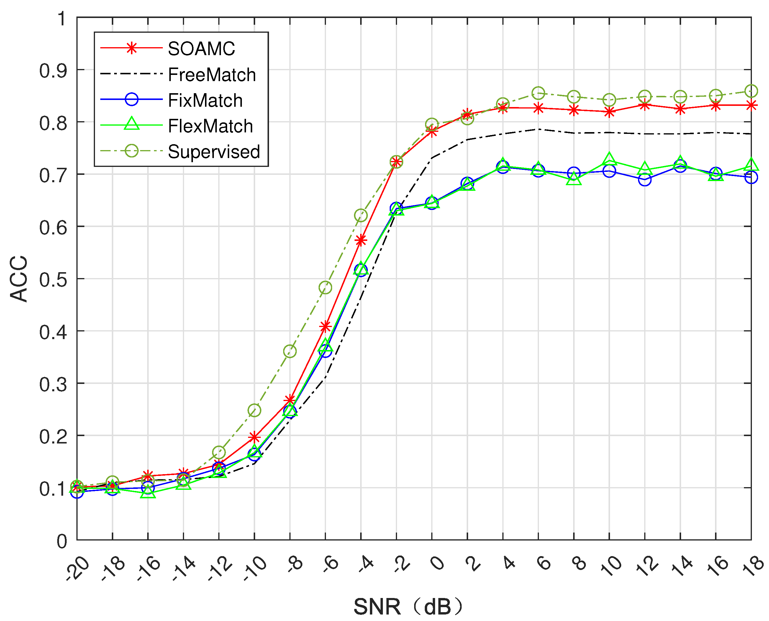
4.2.1. Public Dataset Validation

The validation of this experiment was conducted using the RML2016.10a public dataset. In their study, Javier Maroto et al. [40] identified the issue of AM-SSB signals being obscured by AWGN noise, leading to the deliberate exclusion of AM-SSB signals from the experimental dataset. The dataset comprises ten modulation types, including 8PSK, AM-DSB, BPSK, CPFSK, QFSK, 4PAM, 16QAM, 64QAM, QPSK, and WBFM, encompassing a range of 20 signal-to-noise ratios from −20 dB to 18 dB.

The accuracy curves for the fully supervised learning, FlexMatch algorithm [41], the FixMatch algorithm [16], the FreeMatch algorithm [42], and the SOAMC algorithm proposed in this study are illustrated in Figure 3. By using semi-supervised learning algorithms, a large number of unlabeled modulation signal samples can be utilized for model training, even if only a limited number of labeled samples are available. This method greatly reduces the need for labeled data and improves the efficiency and accuracy of modulation signal recognition. Figure 3 in the experiment also shows a comparison of the recognition accuracy between fully supervised learning and semi-supervised learning. Fully supervised learning is trained using 1000 labeled data in each signal-to-noise ratio of each class. Although the performance of fully supervised learning is better than that of existing semi-supervised learning, our proposed method approaches the performance of fully supervised algorithms by using only a combination of 20 labeled data and 1000 unlabeled data for each signal-to-noise ratio and class. This result demonstrates the effectiveness of the adaptive enhancement module and graph semi-supervised algorithm framework we used. The adaptive enhancement module improves the feature extraction ability of the model for a small amount of data, and can achieve high-performance modulation recognition accuracy with only a small amount of labeled data. This has certain application value for scenarios with fewer labeling costs and fewer samples in practice.

It can be seen from Figure 3 that the recognition accuracy of the FlexMatch algorithm and the FixMatch algorithm is low, especially after 0 dB, and the FlexMatch algorithm and the FixMatch algorithm show a lower recognition rate. The recognition rate of the FreeMatch algorithm is higher than that of the FlexMatch algorithm and the FixMatch algorithm. It can be seen that the FreeMatch adaptive threshold adjustment and adaptive fair regularization multiplication are effective for modulated signal data. The accuracy of the proposed SOAMC algorithm in low SNR and high SNR is significantly higher than that of the FreeMatch algorithm, and it is close to the fully supervised algorithm, which shows the effectiveness of the proposed SOAMC algorithm.

Figure 4a,b depict the recognition accuracy of each modulation mode at various signal-to-noise ratios. A comparison of the two figures reveals that SOAMC demonstrates significant enhancements for the challenging modulation types of WBFM and 16QAM.

The analysis of the confusion matrices presented in Figure 5a,b reveals that the model trained using the FreeMatch algorithm exhibits notably low WBFM recognition accuracy at 0 dB. Specifically, a significant portion of WBFMs are misclassified as AM-DSBs, while a majority of 16QAMs are misclassified as 64QAMs. This deficiency in accurately recognizing WBFMs and 16QAMs primarily contributes to the overall poor performance of the FreeMatch algorithm at 0 dB. Conversely, the model trained with the SOAMC algorithm demonstrates substantial enhancements in the recognition accuracy of WBFM and 16QAM signals at 0 dB. This improvement underscores the efficacy of the optimization scheme proposed in this study, which in turn validates the superiority of the enhanced algorithm introduced herein.

The confusion matrix depicted in Figure 5c,d illustrates that the model trained using the FreeMatch algorithm did not exhibit any enhancement in the recognition accuracy of WBFM and 16QAM signals at 8 dB and 0 dB, as shown in Figure 5a,b. Specifically, a significant portion of WBFM signals were misclassified as AM-DSB, while a considerable number of 16QAM signals were misidentified as 64QAM. This misclassification of WBFM and 16QAM signals primarily contributed to the overall poor recognition accuracy of the FreeMatch algorithm at 10 dB. In contrast, the model trained with the SOAMC algorithm demonstrated notable improvements in the recognition accuracy of WBFM and 16QAM signals at 10 dB. A comparison between Figure 5a,b indicates a substantial increase in the recognition rate of WBFM signals at 10 dB compared to 0 dB. This observation validates that the optimization strategy proposed in this study facilitates an enhanced recognition rate at higher signal-to-noise ratios, aligning more closely with the characteristics of modulated signal data. Consequently, this study affirms the efficacy of the algorithm proposed herein for processing modulated signals.

Figure 6 illustrates a comparison of the recognition rates between FreeMatch and the proposed SOAMC algorithm across varying numbers of labeled samples. When faced with severely limited labeled data, specifically five labeled samples per class per signal-to-noise ratio, the SOAMC method demonstrates a 2% increase in accuracy compared to the FreeMatch approach. Moreover, with only 10 and 20 labeled samples per class per SNR, the SOAMC algorithm exhibits enhanced recognition performance, showcasing accuracy improvements of 4% and 3% over the FreeMatch method, respectively. These results unequivocally establish the superior performance of the proposed method over the FreeMatch technique in scenarios with scarce amounts of labeled data.

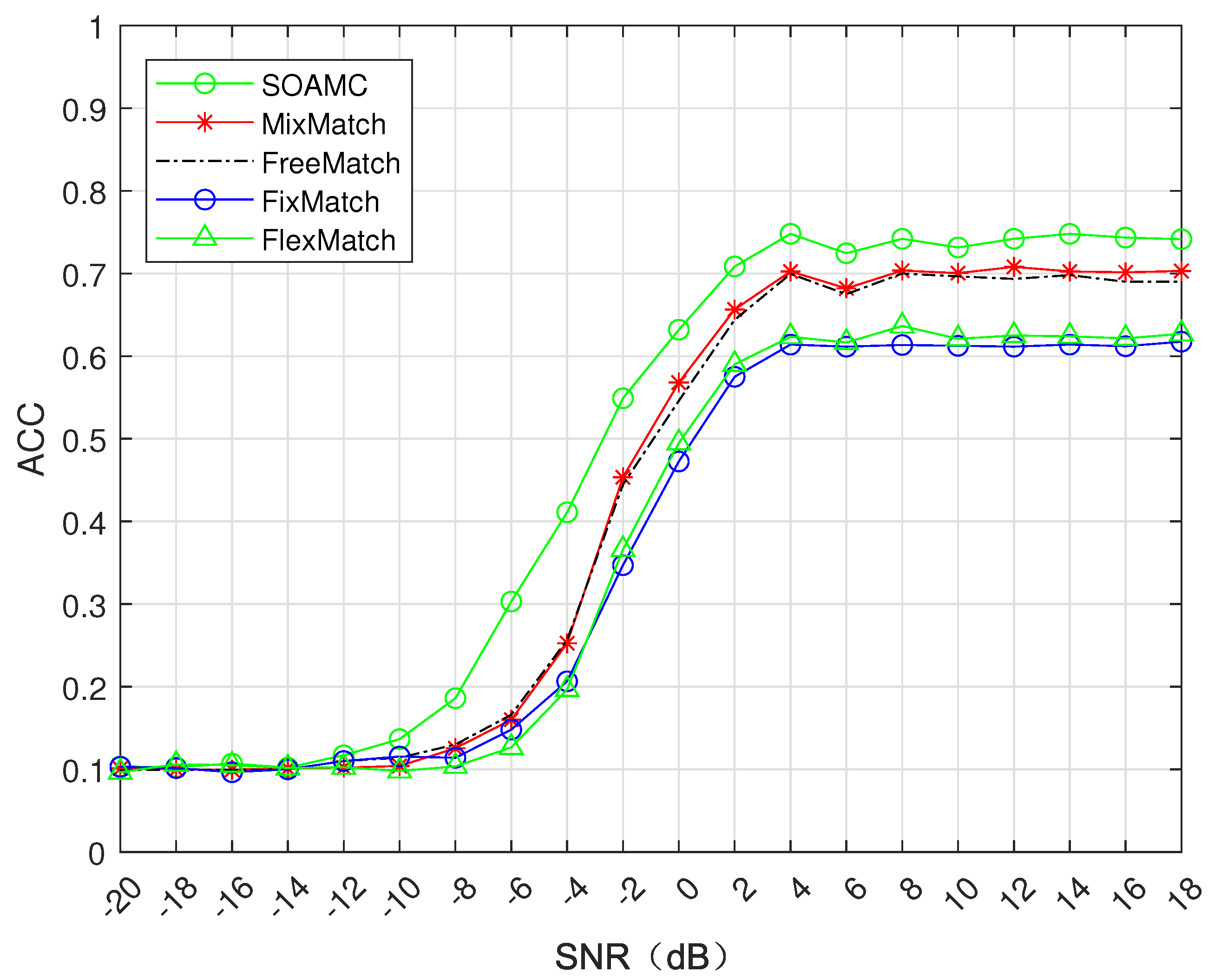
4.2.2. Self-Made Dataset Verification

The accuracy curves depicting the recognition performance of the model on the test set during the training phase of the SOAMC, MixMatch, FreeMatch, FixMatch, and FlexMatch algorithms introduced in this study are illustrated in Figure 7. The training dataset utilized in the model training consists of 30 labeled data instances per class per signal-to-noise ratio, 1000 unlabeled data instances per class per signal-to-noise ratio, and 200 test data instances per class per signal-to-noise ratio, with data distributed across ten classes. Analysis of Figure 7 reveals that the recognition accuracy curves of the FixMatch and FlexMatch algorithms exhibit lower accuracy levels compared to other algorithms. Notably, the SOAMC algorithm consistently outperforms the FreeMatch algorithm across all signal-to-noise ratios, indicating the efficacy of the proposed approach.

We perform a simulation to evaluate the performance of our proposed method under the Rayleigh fading channel. The simulation assumes the symbol rate is 1 Msps, and the maximum Doppler shift for the channel path is set to 30. The simulation results are shown in Figure 8. We can observe that the recognition accuracy of the proposed method experiences fluctuations under high signal-to-noise ratios, but its accuracy still surpasses that of the FixMatch and FlexMatch algorithms.

4.3. Complexity Analysis

In our proposed method, the computational complexity mainly comes from the convolutional neural network, whose structure is shown in

Table 2. Structure of the pre-trained model.

Layers	Output Size	Configuration
Convolution 1	$32\times 512\times 1$	Conv,32,$15\times 2$
Convolution 2	$64\times 255\times 1$	Conv,64,$7\times 1,S=2$
Residual Block 1	$64\times 128\times 1$	$\left[\begin{array}{c}\mathrm{Conv},64,1\times 1\hfill \\ \mathrm{Conv},64,3\times 1,S=2\hfill \\ \mathrm{Conv},64,1\times 1\hfill \end{array}\right]$
Residual Block 2	$64\times 128\times 1$	$\left[\begin{array}{c}\mathrm{Conv},64,1\times 1\hfill \\ \mathrm{Conv},64,3\times 1\hfill \\ \mathrm{Conv},64,1\times 1\hfill \end{array}\right]$
Residual Block 3	$128\times 64\times 1$	$\left[\begin{array}{c}\mathrm{Conv},128,1\times 1\hfill \\ \mathrm{Conv},128,3\times 1,S=2\hfill \\ \mathrm{Conv},128,1\times 1\hfill \end{array}\right]$
Residual Block 4	$128\times 64\times 1$	$\left[\begin{array}{c}\mathrm{Conv},128,1\times 1\hfill \\ \mathrm{Conv},128,3\times 1\hfill \\ \mathrm{Conv},128,1\times 1\hfill \end{array}\right]$
Residual Block 5	$256\times 32\times 1$	$\left[\begin{array}{c}\mathrm{Conv},256,1\times 1\hfill \\ \mathrm{Conv},256,3\times 1,S=2\hfill \\ \mathrm{Conv},256,1\times 1\hfill \end{array}\right]$
Residual Block 6	$256\times 32\times 1$	$\left[\begin{array}{c}\mathrm{Conv},256,1\times 1\hfill \\ \mathrm{Conv},256,3\times 1\hfill \\ \mathrm{Conv},256,1\times 1\hfill \end{array}\right]$
Pooling Layer	$256\times 1\times 1$	Global average pool
Classification	128	Fully connected layer
	64	Fully connected layer
	M	Fully connected layer

. Therefore, we consider using the number of additions and multiplications to measure the complexity of the network.

In the process of the forward propagation of samples in the network, computational complexity is generated. We assume the input of each layer is $h_{in}\times {\mathrm{w}}_{in}\times {\mathrm{w}}_{in}$, and the corresponding output is $h_{out}\times {\mathrm{w}}_{out}\times {\mathrm{w}}_{out}$, then the computational complexity of the convolutional layer is

$$C_{conv}\sim O(c_{in}\times h_{out}\times {\mathrm{w}}_{out}\times {\mathrm{c}}_{out}\times \mathrm{k})$$

where k is the size of the convolution kernel, $c_{in}$ is the channel of input, and $c_{out}$ is the channel of output, i.e., the number of convolution kernels. The computational complexity of the batch normalization layer and the ReLU layer are both

$$C_{bn}\sim O(h_{in}\times {\mathrm{w}}_{in}\times {\mathrm{c}}_{in})$$

The computational complexity of the pooling layer is:

$$C_{pooling}\sim O(h_{out}\times {\mathrm{w}}_{out}\times {\mathrm{c}}_{out}\times p)$$

where the is the kernel size of the pooling layer.

The other part of computational complexity arises in the graph construction and label propagation. We assume that there are three labeled samples corresponding to three incremental classes and one unlabeled sample. Then, the computational complexity includes 3187 multiplications (or divisions), 6184 additions (or subtractions), and 12 exponents, which is much lower than the amount of these in the forward propagation.

Table 3. Computational complexity comparison per testing sample.

Metrics	Ours	FlexMatch
Multiplication and division	38,410,112	44,308,907
Addition and subtraction	38,467,456	44,308,907
Comparator	212,864	258,145

gives out the computational complexity of the forward propagation of one sample in the pre-training model and the compared computational complexity of the FlexMatch method for testing one sample. It can be seen from Table 3 that the computational complexity of our proposed method in the process of forward propagation is lower than that of the FlexMatch method.

5. Conclusions

This paper presents an in-depth analysis of the current development trends and challenges in automatic modulation classification technologies, particularly in open-set scenarios. To address the limitations of existing open-set modulation recognition techniques, we propose a semi-supervised open-set recognition method, SOAMC. By incorporating data augmentation and adaptive adjustment techniques in the pre-training phase, the algorithm enhances its robustness. Furthermore, the designed open-set feature embedding mechanism refines the classification of unknown samples, even in cases where only a limited number of samples are manually labeled. Simulation experiments conducted on both open-source and self-constructed datasets demonstrate the effectiveness of the proposed SOAMC method, highlighting its potential for practical application in open-set modulation recognition.

With the rapid advancement of deep learning technologies, the modulation recognition of communication signals has become increasingly intelligent, fostering the integration of communication systems and deep learning. This convergence has attracted considerable attention and presents new opportunities for further exploration. In light of the research focus and objectives of this study, several promising areas for future research are identified:

•

This paper presents a novel approach to open-set recognition and semi-supervised modulation signal classification, aiming to improve the accuracy of classifying known samples while developing robust rejection mechanisms for samples from unknown classes. However, the subsequent processing and interpretability of rejected samples remain underexplored. Future work could benefit from a deeper investigation into extending open-set recognition tasks by incorporating new class discovery techniques, which would enhance the system’s ability to manage previously unseen modulation types.

•

Furthermore, while the proposed method demonstrates strong performance when a small number of unknown category samples are manually labeled, exploring alternative approaches to identify unknown data without relying on manual labeling is a compelling avenue for future research. This would involve developing fully automated mechanisms to recognize unknown categories, expanding the applicability of the method in more dynamic and real-time communication environments.

References

1. Dobre, O.A.; Abdi, A.; Bar-Ness, Y.; Su, W. Survey of automatic modulation classification techniques: Classical approaches and new trends. IET Commun. 2007, 1, 137–156. [Google Scholar] [CrossRef]
2. Xu, J.L.; Su, W.; Zhou, M. Likelihood-ratio approaches to automatic modulation classification. IEEE Trans. Syst. Man Cybern. Part C (Appl. Rev.) 2010, 41, 455–469. [Google Scholar] [CrossRef]
3. Zhang, Z.; Wang, C.; Gan, C.; Sun, S.; Wang, M. Automatic modulation classification using convolutional neural network with features fusion of SPWVD and BJD. IEEE Trans. Signal Inf. Process. Netw. 2019, 5, 469–478. [Google Scholar] [CrossRef]
4. Zheng, S.; Hu, J.; Zhang, L.; Qiu, K.; Chen, J.; Qi, P.; Zhao, Z.; Yang, X. FM-Based Positioning via Deep Learning. IEEE J. Sel. Areas Commun. 2024, 42, 2568–2584. [Google Scholar] [CrossRef]
5. Zheng, S.; Yang, Z.; Shen, F.W.; Zhang, L.; Zhu, J.; Zhao, Z.; Yang, X. Deep Learning-Based DOA Estimation. IEEE Trans. Cogn. Commun. Netw. 2024, 10, 819–835. [Google Scholar] [CrossRef]
6. Qi, P.; Jiang, T.; Xu, J.; He, J.; Zheng, S.; Li, Z. Unsupervised Spectrum Anomaly Detection with Distillation and Memory Enhanced Autoencoders. IEEE Internet Things J. 2024. [Google Scholar] [CrossRef]
7. Goodfellow, I.; Bengio, Y.; Courville, A. Deep Learning; MIT Press: Cambridge, MA, USA, 2016. [Google Scholar]
8. LeCun, Y.; Bengio, Y.; Hinton, G. Deep learning. Nature 2015, 521, 436–444. [Google Scholar] [CrossRef]
9. Van Engelen, J.E.; Hoos, H.H. A survey on semi-supervised learning. Mach. Learn. 2020, 109, 373–440. [Google Scholar] [CrossRef]
10. Zhou, Z.H.; Zhou, Z.H. Semi-supervised learning. Mach. Learn. 2021, 315–341. [Google Scholar] [CrossRef]
11. Wang, H.; Zhang, Q.; Wu, J.; Pan, S.; Chen, Y. Time series feature learning with labeled and unlabeled data. Pattern Recognit. 2019, 89, 55–66. [Google Scholar] [CrossRef]
12. Simao, M.; Mendes, N.; Gibaru, O.; Neto, P. A review on electromyography decoding and pattern recognition for human-machine interaction. IEEE Access 2019, 7, 39564–39582. [Google Scholar] [CrossRef]
13. Lee, D.H. Pseudo-label: The simple and efficient semi-supervised learning method for deep neural networks. In Workshop on Challenges in Representation Learning; ICML: San Diego, CA, USA, 2013; pp. 1–6. [Google Scholar]
14. Zou, Y.; Yu, Z.; Liu, X.; Kumar, B.; Wang, J. Confidence regularized self-training. In Proceedings of the IEEE/CVF International Conference on Computer Vision, Seoul, Republic of Korea, 27 October–2 November 2019; pp. 5982–5991. [Google Scholar]
15. Mukherjee, S.; Awadallah, A.H. Uncertainty-aware self-training for text classification with few labels. arXiv 2020, arXiv:2006.15315. [Google Scholar]
16. Sohn, K.; Berthelot, D.; Carlini, N.; Zhang, Z.; Zhang, H.; Raffel, C.A.; Cubuk, E.D.; Kurakin, A.; Li, C.L. Fixmatch: Simplifying semi-supervised learning with consistency and confidence. Adv. Neural Inf. Process. Syst. 2020, 33, 596–608. [Google Scholar]
17. Cubuk, E.D.; Zoph, B.; Shlens, J.; Le, Q.V. Randaugment: Practical automated data augmentation with a reduced search space. In Proceedings of the IEEE/CVF Conference on Computer Vision and Pattern Recognition Workshops, Seattle, WA, USA, 14–19 June 2020; pp. 702–703. [Google Scholar]
18. Xie, Q.; Dai, Z.; Hovy, E.; Luong, T.; Le, Q. Unsupervised data augmentation for consistency training. Adv. Neural Inf. Process. Syst. 2020, 33, 6256–6268. [Google Scholar]
19. Deng, L.; Yu, D. Deep learning: Methods and applications. Found. Trends® Signal Process. 2014, 7, 197–387. [Google Scholar] [CrossRef]
20. He, K.; Zhang, X.; Ren, S.; Sun, J. Deep residual learning for image recognition. In Proceedings of the IEEE Conference on Computer Vision and Pattern Recognition, Las Vegas, NV, USA, 27–30 June 2016; pp. 770–778. [Google Scholar]
21. Zhang, C.; Bengio, S.; Hardt, M.; Recht, B.; Vinyals, O. Understanding deep learning (still) requires rethinking generalization. Commun. ACM 2021, 64, 107–115. [Google Scholar] [CrossRef]
22. Gui, G.; Huang, H.; Song, Y.; Sari, H. Deep learning for an effective nonorthogonal multiple access scheme. IEEE Trans. Veh. Technol. 2018, 67, 8440–8450. [Google Scholar] [CrossRef]
23. Zhang, Y.; Doshi, A.; Liston, R.; Tan, W.t.; Zhu, X.; Andrews, J.G.; Heath, R.W. DeepWiPHY: Deep learning-based receiver design and dataset for IEEE 802.11 ax systems. IEEE Trans. Wirel. Commun. 2020, 20, 1596–1611. [Google Scholar] [CrossRef]
24. Ghasemzadeh, P.; Banerjee, S.; Hempel, M.; Sharif, H. A novel deep learning and polar transformation framework for an adaptive automatic modulation classification. IEEE Trans. Veh. Technol. 2020, 69, 13243–13258. [Google Scholar] [CrossRef]
25. Lyu, Z.; Wang, Y.; Li, W.; Guo, L.; Yang, J.; Sun, J.; Liu, M.; Gui, G. Robust automatic modulation classification based on convolutional and recurrent fusion network. Phys. Commun. 2020, 43, 101213. [Google Scholar] [CrossRef]
26. Weng, L.; He, Y.; Peng, J.; Zheng, J.; Li, X. Deep cascading network architecture for robust automatic modulation classification. Neurocomputing 2021, 455, 308–324. [Google Scholar] [CrossRef]
27. Zhang, H.; Nie, R.; Lin, M.; Wu, R.; Xian, G.; Gong, X.; Yu, Q.; Luo, R. A deep learning based algorithm with multi-level feature extraction for automatic modulation recognition. Wirel. Netw. 2021, 27, 4665–4676. [Google Scholar] [CrossRef]
28. Shang, J.; Sun, Y. Predicting the hosts of prokaryotic viruses using GCN-based semi-supervised learning. BMC Biol. 2021, 19, 250. [Google Scholar] [CrossRef]
29. Ju, Y.; Gao, Z.; Wang, H.; Liu, L.; Pei, Q.; Dong, M.; Mumtaz, S.; Leung, V.C.M. Energy-efficient cooperative secure communications in mmwave vehicular networks using deep recurrent reinforcement learning. IEEE Trans. Intell. Transp. Syst. 2024, 25, 14460–14475. [Google Scholar] [CrossRef]
30. Ju, Y.; Cao, Z.; Chen, Y.; Liu, L.; Pei, Q.; Mumtaz, S.; Dong, M.; Guizani, M. Noma-assisted secure offloading for vehicular edge computing networks with asynchronous deep reinforcement learning. IEEE Trans. Intell. Transp. Syst. 2024, 25, 2627–2640. [Google Scholar] [CrossRef]
31. Li, C.; Guan, L.; Wu, H.; Cheng, N.; Li, Z.; Shen, X.S. Dynamic spectrum control-assisted secure and efficient transmission scheme in heterogeneous cellular networks. Engineering 2022, 17, 220–231. Available online: https://www.sciencedirect.com/science/article/pii/S2095809921002666 (accessed on 17 October 2024). [CrossRef]
32. Han, H.; Ma, W.; Zhou, M.; Guo, Q.; Abusorrah, A. A novel semi-supervised learning approach to pedestrian reidentification. IEEE Internet Things J. 2020, 8, 3042–3052. [Google Scholar] [CrossRef]
33. Khonglah, B.; Madikeri, S.; Dey, S.; Bourlard, H.; Motlicek, P.; Billa, J. Incremental semi-supervised learning for multi-genre speech recognition. In Proceedings of the ICASSP 2020-2020 IEEE International Conference on Acoustics, Speech and Signal Processing (ICASSP), Barcelona, Spain, 4–8 May 2020; IEEE: Piscataway, NJ, USA, 2020; pp. 7419–7423. [Google Scholar]
34. O’Shea, T.J.; Corgan, J.; Clancy, T.C. Unsupervised representation learning of structured radio communication signals. In Proceedings of the 2016 First International Workshop on Sensing, Processing and Learning for Intelligent Machines (SPLINE), Aalborg, Denmark, 6–8 July 2016; IEEE: Piscataway, NJ, USA, 2016; pp. 1–5. [Google Scholar]
35. O’Shea, T.J.; West, N.; Vondal, M.; Clancy, T.C. Semi-supervised radio signal identification. In Proceedings of the 2017 19th International Conference on Advanced Communication Technology (ICACT), Pyeongchang, Republic of Korea, 19–22 February 2017; IEEE: Piscataway, NJ, USA, 2017; pp. 33–38. [Google Scholar]
36. O’shea, T.J.; West, N. Radio machine learning dataset generation with gnu radio. In Proceedings of the GNU Radio Conference, Boulder, CO, USA, 12–16 September 2016; Volume 1. [Google Scholar]
37. Zhang, M.; Zeng, Y.; Han, Z.; Gong, Y. Automatic modulation recognition using deep learning architectures. In Proceedings of the 2018 IEEE 19th International Workshop on Signal Processing Advances in Wireless Communications (SPAWC), Kalamata, Greece, 25–28 June 2018; IEEE: Piscataway, NJ, USA, 2018; pp. 1–5. [Google Scholar]
38. Zheng, S.; Qi, P.; Chen, S.; Yang, X. Fusion methods for CNN-based automatic modulation classification. IEEE Access 2019, 7, 66496–66504. [Google Scholar] [CrossRef]
39. Chen, S.; Zhang, Y.; He, Z.; Nie, J.; Zhang, W. A novel attention cooperative framework for automatic modulation recognition. IEEE Access 2020, 8, 15673–15686. [Google Scholar] [CrossRef]
40. Huynh-The, T.; Pham, Q.V.; Nguyen, T.V.; Nguyen, T.T.; Ruby, R.; Zeng, M.; Kim, D.S. Automatic modulation classification: A deep architecture survey. IEEE Access 2021, 9, 142950–142971. [Google Scholar] [CrossRef]
41. Zhang, B.; Wang, Y.; Hou, W.; Wu, H.; Wang, J.; Okumura, M.; Shinozaki, T. Flexmatch: Boosting semi-supervised learning with curriculum pseudo labeling. Adv. Neural Inf. Process. Syst. 2021, 34, 18408–18419. [Google Scholar]
42. Wang, Y.; Chen, H.; Heng, Q.; Hou, W.; Fan, Y.; Wu, Z.; Wang, J.; Savvides, M.; Shinozaki, T.; Raj, B.; et al. Freematch: Self-adaptive thresholding for semi-supervised learning. arXiv 2022, arXiv:2205.07246. [Google Scholar]
Figure 1. The structure of the SOAMC framework. The adaptive enhancement module utilizes data enhancement and threshold adjustment techniques to pre-train signal feature extraction networks. Open-set features are embedded in the pre-training network, then features are extracted using the fine-tuning network, and features are fed into a graph neural network for label propagation.
Electronics 13 04196 g001
Figure 2. Recognition accuracy of SOAMC algorithm in open-set scenarios.
Electronics 13 04196 g002
Figure 3. Accuracy comparison chart of 20 labeled data for each class and SNR.
Electronics 13 04196 g003
Figure 4. The recognition accuracy of each modulation at each SNR, in which SOAMC has a performance improvement over FreeMatch. (a) The SOAMC recognition accuracy chart. (b) The FreeMatch recognition accuracy chart.
Electronics 13 04196 g004
Figure 5. Comparison of results between SOAMC and FreeMatch split on 0 dB and 8 dB on the confusion matrix. (a) FreeMatch—0 dB. (b) SOAMC—0 dB. (c) FreeMatch—8 dB. (d) SOAMC—8 dB.
Electronics 13 04196 g005
Figure 6. Comparison of the recognition accuracy of different numbers of labeled data.
Electronics 13 04196 g006
Figure 7. Recognition accuracy curves of the SOAMC, MixMatch, FreeMatch, FixMatch and FlexMatch algorithms for the test set of the model during training.
Electronics 13 04196 g007
Figure 8. Recognition accuracy curves of the SOAMC, MixMatch, FreeMatch, FixMatch and FlexMatch algorithms for the test set under the Rayleigh fading channel.
Electronics 13 04196 g008