Improving Recognition of Road Users via Doppler Radar Data and Deep Learning Convolutional Networks

Abstract

This research presents findings from laboratory experiments on a novel method for identifying and differentiating objects using radar signatures and a specialized convolutional neural network architecture. Previously introduced by the authors, this method has been validated through real-world measurements in an urban environment with a 24 GHz frequency-modulated continuous-wave radar. This study describes how radar signatures, generated in the MATLAB (R2023b) environment from I and Q signals captured by the uRAD USB v1.2 radar, were processed. A database of radar signatures for pedestrians, cyclists, and vehicles was created, and a tailored convolutional neural network was trained. The developed solution achieves an accuracy of over 95% in distinguishing between various objects. The simulation results and successful tests support the application of this system across various sectors. The key innovations include distinguishing multiple objects from a single radar signature, a custom architecture for the convolutional neural network, and an application that processes radar data to produce near-real-time recognition results.

1. Introduction

The classification of people and vehicles is a key element in accident prevention in autonomous vehicle driving. Radar-sensor-based classification techniques in the automotive field have gained increased attention from researchers due to their robustness in low-light conditions and adverse weather [1].

Deep learning, as a branch of artificial intelligence, plays a key role in the development of modern automotive technologies. Examples of its applications include autonomous driving systems that rely on advanced machine learning algorithms for object recognition, real-time decision-making, and route planning [2]. Deep learning is based on multi-layered neural networks that perform two main functions [3]. The first main function of neural networks, which is generating diagnostic features, allows the model to autonomously identify relevant patterns and characteristics that may be key to solving a given problem. This makes the machine learning process less dependent on the manual definition of features by experts, which in traditional methods often requires extensive specialized knowledge and intuition. In practice, the neural network learns to detect and recognize the features that best describe the analyzed process. The second function, classification or regression, involves assigning input data to one of many categories (classification) or predicting a continuous value (regression). This approach is extremely useful in the automotive field, where neural networks can be used for recognizing objects on the road, predicting the trajectories of other vehicles, or optimizing fuel consumption. Thus, deep learning enables the automation of many complex tasks that were previously reserved for humans, such as fault diagnostics or the interpretation of sensory data [4].

The use of deep neural networks for analyzing radar data can significantly change the way they are applied, especially in complex operational environments. Automating the interpretation of radar imagery enables the faster and more efficient detection and classification of objects, reducing the need for human intervention [1]. Radars have an advantage over traditional sensors as they operate effectively in challenging atmospheric conditions, such as fog or rain, where other sensors may fail. Although radars can be easily detected by adversaries, advanced signal processing techniques can minimize the risk of detection [5]. Neural networks can achieve higher detection accuracy by learning from large datasets, which enhances their effectiveness in various terrain and atmospheric conditions. Their ability to adapt to dynamically changing environments is crucial in military applications, in which situations can evolve rapidly. Consequently, the authors suggested a solution that substitutes the complex analysis of radar images by employing deep neural networks to distinguish between various types of objects moving towards the radar [6].

The micro-Doppler effect, which occurs when an object illuminated by radar waves makes small movements, such as vibrations, rotations, or mechanical oscillations, generates characteristic radar signatures [7]. These signatures are unique to each object as they reflect the specific movements of its parts, such as the rotation of helicopter blades, the movements of human limbs while walking, or the operation of an aircraft engine components [8]. The use of these micro-Doppler signatures as input data for convolutional neural networks (CNNs) opens up new possibilities in the analysis and identification of objects.

Convolutional neural networks are exceptionally effective at pattern recognition and image analysis, allowing them to process micro-Doppler signatures as radar images, identifying features characteristic of different types of objects and their movements. The neural network learns to recognize unique patterns associated with the micro-movements of the object, enabling accurate classification and identification even in challenging conditions, such as low visibility or interference [9]. This combination of micro-Doppler data with convolutional neural networks enables the automation and acceleration of radar analysis, enhancing precision and efficiency when detecting objects with various motion characteristics.

In [6], the authors of this article introduced a novel approach based on simulated data generated in the MATLAB environment, along with an innovative method for object identification using a 77 GHz FMCW radar. The approach involves processing the acquired signals with Short-Time Fourier Transform (STFT), followed by analyzing the resulting spectrograms with a tailored deep neural network architecture.

To validate the developed method, the authors conducted a series of laboratory tests using the uRAD USB v1.2 radar with a continuous wave modulated at a frequency of 24 GHz. Furthermore, a series of simulation experiments were conducted for pedestrian, cyclist, and vehicle models within the MATLAB environment, using a radar operating at a frequency of 24 GHz, as opposed to the 77 GHz radar referenced in the study [6].

The innovative contributions in this article include the following:

• The development of an object recognition method utilizing a FMCW radar, in which the acquired signals are processed using STFT, followed by analyzing the resulting spectrograms with deep neural networks;
• The creation of a technique for generating and processing simulated radar data;
• The formulation of a method for producing spectrograms from raw FMCW radar signals;
• The development of an application that processes radar data (prepared spectrograms) and generates recognition results based on a dedicated convolutional neural network in near-real time.

This article is structured as follows: the second section reviews the current state of knowledge on the topics discussed. The third section explains the method for generating the radar data to be used as inputs for a specialized convolutional neural network, the process for creating spectrograms from raw FMCW radar signals, as well as an application for processing radar data and producing recognition results using a tailored convolutional neural network in near-real time. This section also includes a concise overview of the FMCW radar, object models, Fourier transform (STFT), and a description of the convolutional neural network architecture and parameters. The fourth section presents the experimental results, while the fifth section offers conclusions and discussions on the findings.

2. Related Works

In the process of processing radar data, micro-Doppler signatures are often represented using spectrograms—graphical representations of signal frequency changes over time. Such spectrograms contain data regarding particular motion patterns, which are subsequently analyzed by deep learning algorithms, including CNNs. Numerous instances of detecting and classifying individuals, animals, or vehicles in this way have been showcased in the authors’ previous research [6]. This paper offers additional examples to emphasize the existing gap in the literature related to the topics addressed in the authors’ scientific work in this article.

The beginnings of using neural networks as the main classifier can be traced back to 1996. In article [10], a method for classifying aircraft based on the modulation of their engine operation using radar that received signals reflected from the planes was proposed. Optical Fourier transformation was used to extract the engine modulation signatures. A semi-connected neural network with a backpropagation algorithm (BPNN) consisting of three layers was applied for classification.

More contemporary results related to this topic include the works [11,12]. Study [11] analyzes the use of neural networks in the classification of radar targets using Forward Scattering Radar (FSR). It focuses on classifying road vehicles, with features extracted from raw radar signals being manually processed and analyzed by a Multi-Layer Perceptron (MLP) neural network with a backpropagation algorithm. Two types of classification were evaluated: determining the type of vehicle and grouping vehicles by category. The results show that the proposed neural network outperforms the k-nearest neighbors classifier in terms of classification accuracy. In article [12], a neural-network-based classifier for classifying airborne radar targets is proposed. The classification relies on features extracted from RCS time series and their corresponding Intrinsic Mode Functions (IMFs). Comparisons of the results demonstrated that the proposed classifier is more effective than other methods for the same data. A common trend in these studies is the use of very small data samples (tens or hundreds) and very shallow networks (3–4 layers).

In paper [13], shallow (two- and six-layer) CNNs were used to classify objects based on their radar reflections. The authors conducted their analysis using approximately 4000 samples of signals reflected from unmanned aerial vehicles (UAVs), people, cars, and other objects, achieving classification accuracies of 32.10% for UAVs, 72.59% for people, and 43.58% for cars. The study employed a data augmentation method to increase the volume of input data.

In article [14], the authors tackled the challenges of aircraft classification and outlier removal using high-resolution radar (HRR) data and a CNN neural network architecture. This architecture comprises two primary components, a classifier and a decoder, which is employed to eliminate invalid targets. The research demonstrated that the classification accuracy is influenced by the network architecture, the quantity of training data, and hyperparameter configurations, yet in all cases, it reached a value exceeding 90%. Around 100,000 samples were utilized for training, which is considerably more than in other studies on this subject.

Hadhrami [15] introduced a novel method for classifying moving ground targets by employing pre-trained CNN models for feature extraction. The VGG16 and VGG19 models were used for this purpose, while classification was carried out using support vector machines (SVM). Radar spectrogram images provided the input data for the VGG models. The experiment incorporated all eight classes from the RadEch database. The features extracted from the 14th layer (fc6) of the VGG16 model attained the highest classification accuracy, of 96.56%.

In article [16], the results of classifying various target classes (car, single and multiple people, bicycle) using radar data from an automotive radar and different neural network architectures are presented. Fast radar algorithms for detection, tracking, and micro-Doppler extraction are proposed, working in conjunction with the TEF810X radar transceiver and the SR32R274 microcontroller unit from NXP Semiconductors (Eindhoven, Netherlands). Three types of neural networks were considered: a classical convolutional network, a residual network, and a combination of convolutional and recurrent networks. The results demonstrated high classification accuracy (nearly 100% in some cases) and low preprocessing latency (approximately 0.55 s for a 0.5 s spectrogram). Although based on a small experimental data sample, these results highlighted the benefits (high accuracy) and potential drawbacks (overfitting, lack of generalization robustness) of various network architectures. The findings suggest that collecting larger experimental datasets and improving radar architecture and radar signal processing could enhance classification results. Additionally, implementing networks in low-level languages such as C++ could speed up classification time and reduce latency.

The study [17] explores a hybrid method for classifying vehicles and pedestrians in the realm of autonomous driving, employing a combination of Support Vector Machine (SVM) and CNN. This approach addresses the class imbalance issue, wherein the number of detected vehicles considerably exceeds that of pedestrians. In the initial phase, a modified SVM technique based on physical characteristics is utilized to identify vehicles and mitigate data imbalances. The remaining unclassified images are then fed into the CNN. In the second phase, a weighted loss function is implemented to enhance classification performance for the minority class. This method capitalizes on both the localization of features in range-Doppler images and the automatic feature learning capabilities of the CNN, thereby improving classification efficiency. The experimental results indicate that the proposed approach attained high performance, achieving an F1 score of 0.90 and an AUC ROC of 0.99, outperforming other cutting-edge methods with a limited dataset from a 77 GHz radar. The experiment employed a 77 GHz automotive radar along with a Texas Instruments (TI) IRW1443 evaluation board for data acquisition.

In another example [18], an optimization of radar data preprocessing using a parametric CNN is proposed. This method is applied to classify human activities. The proposed parametric CNN uses 2D sinc or 2D wavelet filters to extract features from radar data, improving feature representation and classification results compared to traditional CNN architectures based on Doppler spectrograms or radar data. The preprocessing in the parametric CNN is adaptive and can adjust to signal disturbances. This approach exhibits improved classification accuracy, particularly when there is a limited number of training samples. The reported classification accuracy for different human activities (such as walking, standing still, hand gestures, etc.) in a controlled experimental setting exceeded 0.99, outperforming other cutting-edge methods referenced in the publication.

Table 1. Comparative summary of related works on radar data processing and classification.

Study	Methodology	Main Focus	Data Sample Size	Classification Accuracy	Key Findings
[11]	Multi-Layer Perceptron (MLP) with manual feature processing	Classifying road vehicles	Not specified	Better than k-NN	Manual feature extraction, small data samples
[12]	Neural-network-based classifier	Classifying airborne radar targets	Not specified	More effective than other methods	Uses RCS time series and IMFs
[13]	Shallow CNNs (2–6 layers)	Object classification based on radar reflections	~4000	32.10% (UAV), 72.59% (people), 43.58% (cars)	Data augmentation used to increase input volume
[14]	CNN architecture for HRR data	Aircraft classification and outlier removal	~100,000	>90%	Accuracy influenced by architecture and training data
[15]	Pre-trained CNN models (VGG16, VGG19)	Classifying moving ground targets	All eight classes from RadEch	96.56% (best accuracy)	SVM used for classification
[16]	Various neural network architectures	Classifying target classes (cars, people, bicycles)	Small sample size	Nearly 100% in some cases	Highlights overfitting risks and need for larger datasets
[17]	Hybrid SVM and CNN approach	Classifying vehicles and pedestrians	Limited dataset	F1 score of 0.90, AUC ROC of 0.99	Addresses class imbalance, high performance
[18]	Parametric CNN with 2D sinc/wavelet filters	Classifying human activities	Not specified	>0.99	Improved feature representation and classification accuracy

compares different studies regarding their methodologies, main focuses, data sample sizes, classification accuracies, and key findings, providing a clear overview of the related works on radar data processing and classification.

Taking into account the aforementioned literature review, the authors of this article introduced a novel approach based on simulated data generated in the MATLAB environment and a dataset gathered by the uRAD USB v1.2 radar operating at a frequency of 24 GHz, alongside an innovative object recognition method constructed on a specialized deep neural network architecture, where the input data comprise spectrograms acquired through STFT transformation. The key properties of the new approach are as follows:

• The detection of a broader class of objects, such as two pedestrians walking simultaneously or the concurrent movement of a pedestrian and a cyclist in open-space conditions;
• Feature extraction and the classification of images represented as spectrograms for multiple object classes through a specialized CNN;
• A specialized CNN capable of achieving very high object detection accuracy (>90%);
• A CNN that is resistant to overfitting, which is a situation in which the CNN model fits the training data too well but loses the ability to generalize to new, unseen data;
• A solution based on numerical simulations using a simulated dataset in the form of spectrograms (for radars operating at frequencies of 24 GHz and 77 GHz);
• The validation of the numerical solution based on our own dataset from an available FMCW radar operating at a frequency of 24 GHz;
• The use of data augmentation techniques to overcome the challenges and time-consuming nature of processing data from a single FMCW radar measurement.

The drawbacks of our solution include the requirement for a large input dataset and the time-consuming process of building the neural network structure to achieve the highest possible accuracy, as transfer learning techniques were not utilized.

3. System Design and Implementation

This section mainly focuses on the uRAD USB v1.2 radar, which operates at a frequency of 24 GHz, making it suitable for various applications, including short-range surveillance and target detection. This radar system is designed to provide high-resolution data, enabling accurate measurements of distance and speed.

In addition to discussing the radar’s specifications, this section elaborates on the specialized software that facilitates its operation. This software plays a crucial role in configuring the radar parameters, collecting data, and processing the received signals. It provides users with an intuitive interface for real-time monitoring and control, ensuring optimal performance during radar operations.

Furthermore, this section explains the process of transforming raw radar echo signals into spectrograms using the Short-Time Fourier Transform (STFT). This technique involves analyzing radar signals in small time windows, allowing for a detailed frequency representation of the signals over time. By applying STFT, this section illustrates how the radar can effectively visualize the frequency components of the received signals, which aids in identifying and distinguishing between different targets within the radar’s operational environment. This transformation is essential for enhancing the interpretability of radar data, ultimately leading to improved decision-making in various applications.

3.1. Frequency-Modulated Continuous-Wave Radar

Frequency-Modulated Continuous-Wave (FMCW) radar emits a continuous-wave signal with a frequency that changes over time, usually in a linear fashion (LFM). By analyzing the frequency differences between the transmitted and received signals, the radar can determine the distance and speed of objects. Continuous frequency modulation provides two main advantages for FMCW radar. The first advantage is high resolution in measuring distance and speed, allowing for precise differentiation between nearby and fast-moving objects. Second, it is less susceptible to interference from other electromagnetic sources, enhancing its reliability in challenging environmental conditions [19].

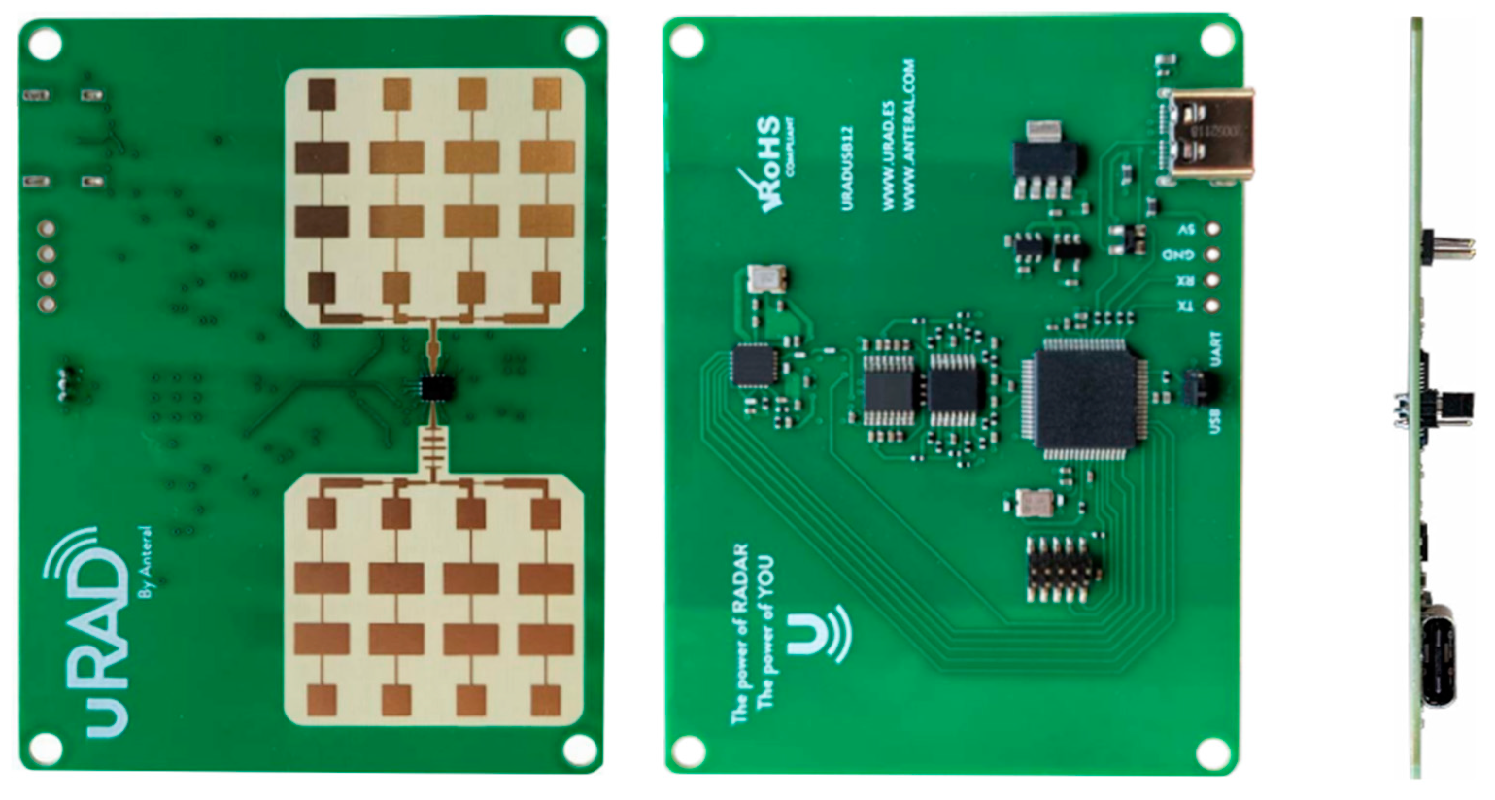
The radar used for this research is the uRAD USB v1.2, operating at a frequency of 24 GHz. The dimensions of the radar are 56 mm × 76 mm × 5 mm.

The uRAD USB v1.2 module is a fully functional microwave FMCW radar, as shown in Figure 1, operating in the 24 GHz band (24.005–24.245 GHz). The USB version allows it to be connected to any device with a USB port. With an array of 16 receiving antennas and 16 transmitting antennas, the radar has a field of view of 30° in both the horizontal and the vertical planes. The radar operates on a power supply of 5 V (USB) and can function in temperature ranges from −20 to +65 °C. The device has four operating modes, which are summarized in

Table 2. Performance characteristics of uRAD USB v1.2.

Mode	1	2	3	4
Waveform	CW (Continuous-wave)	Sawtooth	Triangular	Dual rate
Measured parameters	velocity	Distance	Velocity and distance	Velocity and distance
Distance range (m)	0.45 to 60	0.45 to 100	0.45 to 100	0.45 to 75
Distance resolution (m)	-	max. ±0.04 m or ±0.3%	Max. ±0.04 m or ±0.3%	max. ±0.04 m or ±0.3%
Velocity range (m/s)	±0.7 to ±75	-	±0.2 to ±75	±0.2 to ±75
Velocity resolution (m/s)	3	-	Different distance or 3	Different distance or 3
Update rate max. (samples/second)	103	69	39	20

.

The signal emitted by the FMCW radar is referred to as a chirp. In signals with linear frequency modulation (LFM), the frequency typically changes upward (up-chirp) or downward (down-chirp), and the range of these changes is referred to as the bandwidth [20]. A commonly used solution is to combine the up-chirp and down-chirp signals, resulting in a triangular waveform. The following Figure 2 depicts the chirp signal model produced by the FMCW radar, emphasizing its essential parameters. The subsequent Figure 3 displays the signal waveform graphs for all four operational modes of the uRAD USB v1.2 radar.

The frequencies of the emitted signal over time can be represented as follows [20]:

$$f\left(t\right)=\beta t^{\prime }$$

(1)

where $\beta ={\displaystyle \frac{B}{T}}$ is referred to as the frequency slope, T represents the duration of the chirp, B indicates the frequency bandwidth traversed, $t^{\prime }\in \left[0,T\right],$ and $k=0,\dots ,K-1$. Therefore, the signal emitted by the FMCW radar can be modeled as follows [20]:

$$s\left(t\right)=\cos \left(2\pi f_{C}t+\phi \left(t\right)\right)$$

(2)

where the time t and the phase $\phi \left(t\right)$ are given as follows [20]:

$$t=kT+t^{\prime }$$

(3)

$$\phi \left(t\right)=\pi k\beta T^2+\pi \beta t^{\prime 2}$$

(4)

The relationship for the signal reflected from an object can be expressed as follows [20]:

$$y(t)\approx \epsilon e^{-j2\pi f_B{t}^{\prime }}{e}^{-j2\pi f_{D}kT}$$

(5)

where $\epsilon$ signifies the complex coefficient dependent on gain, $f_B$ indicates the beat frequency, and $f_D$ represents the Doppler frequency. The radar’s receiving pathway is responsible for multiplying the received signal with a replica of the transmitted signal and for filtering it. Finally, knowing the values of $f_B$ and $f_D$, one can ascertain the speed and distance to the object, respectively [21]:

$$V={\displaystyle \frac{f_{D}c}{2f_c}}$$

(6)

$$R={\displaystyle \frac{f_{B}c}{2\beta }}$$

(7)

where c denotes the speed of light.

The echo signal received by the FMCW radar, known as the radio frequency (RF) signal, is quite challenging to analyze because it does not contain complete information about the object. To achieve better analysis quality, the RF signal is transformed into a complex quadrature signal (IQ). This process is called quadrature demodulation (IQ demodulation). IQ data, also known as raw data, are more useful for further analysis. The IQ signal consists of two components: the in-phase component (“I”) represents the real part of the signal, while the quadrature component (“Q”) corresponds to the imaginary part. After quadrature demodulation, the discrete complex signal Z[n] takes the form of

$$Z\left[n\right]=I\left[n\right]+jQ\left[n\right]$$

(8)

In this form, the signal contains information about the amplitude, represented by the I component, and about the phase of the signal, contained in the Q component.

The device manufacturer provides software that allows the user to visualize processed data in real time, as well as to record IQ data from the measurements taken. The view of the radar control application window is shown in the Figure 4 below.

3.2. Data Generation

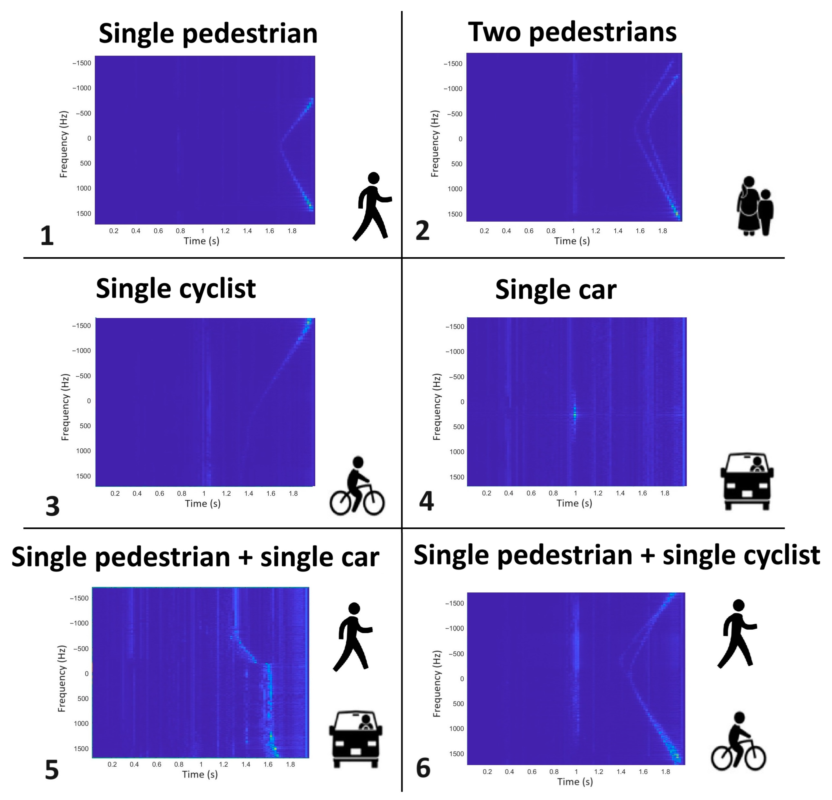
In article [6], the authors presented a method for generating radar data in the MATLAB environment for models of pedestrians, cyclists, and cars, as well as their combinations. For the purpose of research using the uRAD USB v1.2 radar, six scenarios for generating input data were adopted, which correspond to the six classes of objects that the finished system will recognize. For practical research as well as simulations, the following cases were considered when an object is located in front of the radar:

• A single pedestrian;
• Two pedestrians;
• A single cyclist;
• A single car;
• A single pedestrian and a single car;
• A single pedestrian and a single cyclist.

Raw data from the radar are saved to two text files. The first contains the I component of the echo signal, while the second contains the Q component. The structure of the text file depends on the radar’s operational parameters. The number of rows in the file depends on the duration of the measurement, while the number of columns depends on the chosen value of the number of samples taken from the echo signal. Each row in the last two columns contains information about the date and time when the echo signal was received. The value of a single sample represents the voltage received by the radar. After processing by a 12-bit analog-to-digital converter, the values stored in the file range from 0 to 4095, corresponding to voltages of −1 [V] and 1 [V].

Taking the above into consideration, software was developed in the MATLAB environment to convert raw data from text files into spectrograms using the STFT transformation. The illustration of the input data generation for the neural network is shown in the Figure 5 below.

The spectrograms obtained in this way for the 6 cases created a database for further research. Ultimately, the image database comprised 1000 images for each of the 6classes, with each image measuring 875 × 656. Examples of images representing all 6 classes are displayed in Figure 6. Due to the demanding and expensive nature of data collection and labeling, artificial additional training samples were created. For this purpose, geometric transformations, such as image shifts by a specified number of pixels and scaling, were applied in the MATLAB environment.

In addition to geometric transformations, operations on pixel values, such as adding noise, adjusting brightness, and contrast, were also performed. These methods proved to be effective techniques for increasing the training set, leading to improved performance of deep neural networks.

3.3. Short-Time Fourier Transform (STFT)

Short-Time Fourier Transform (STFT) is often used for the analysis of audio signals, speech, radar signals, and other data that change dynamically over time. Unlike the standard Fourier Transform, which provides information about frequencies present in the entire signal, STFT allows for the extraction of frequency information from short segments of the signal. STFT divides the signal into short, overlapping time windows. Each time window is subjected to the classical Fourier Transform, enabling the retrieval of frequency information at a given moment. The result of STFT is a spectrogram—a two-dimensional plot in which the time axis shows how the signal evolves, and the frequency axis presents the frequency distribution for each time window. Colors or intensities on the plot represent the amplitudes of the signal.

The definition of this transformation in the time and frequency domains is as follows [6]:

$${STFT}_x^T\left(t,f\right)=\underset{-\infty }{\overset{+\infty }{\int }}x\left(\tau \right){\gamma }^{*}\left(\tau -t\right)e^{-j2\pi ft}d\tau$$

(9)

$${STFT}_x^F\left(t,f\right)=e^{-j2\pi ft}\underset{-\infty }{\overset{+\infty }{\int }}X\left(\upsilon \right){\Gamma }^{*}\left(\upsilon -f\right)e^{j2\pi \upsilon t}d\upsilon$$

(10)

where the function $\gamma \left(t\right)$ represents the time observation window, and $\Gamma \left(f\right)$ is its Fourier spectrum. For the Short-Time Fourier Transform, the so-called spectrogram is defined as the square of its magnitude [6]:

$$S_x^{SPECTOGRAM}\left(t,f\right)={\left|{STFT}_x\left(t,f\right)\right|}^2$$

(11)

3.4. Deep Learning Network

This article discusses the use of a deep structured CNN model, which has multiple layers responsible for various stages of data processing. The initial layers of the model include convolutional connections, allowing for efficient feature extraction from the input data. The model also employs batch normalization layers, which help accelerate the learning process and stabilize the network’s performance [22]. Additionally, pooling layers are used to reduce the dimensionality of the data and increase resilience to object shifts in the input data. These features create a complex CNN architecture, enabling effective data classification, as illustrated in Figure 7.

The accompanying diagram illustrates the structure of the deep CNN employed for classifying radar data. The process begins with the input layer, which contains Doppler spectrogram images. The network then passes through several convolutional layers with ReLU activation functions and pooling layers that perform max-pooling operations, reducing the dimensionality of the data. After feature extraction, the data are passed to a flattening layer and then to fully connected layers, and the classification process occurs at the output using the softmax function, which assigns probabilities to individual classes, such as cyclist, pedestrian, or vehicle. The structure of the CNN, built from scratch in MATLAB, included four convolutional layers, defined after a series of preliminary experiments [23]:

• First layer: 16 neurons, filter with a receptive field of 5 × 5, stride of 2 × 2, batch normalization, ReLU activation function, max pooling;
• Second layer: 32 neurons, filter with a receptive field of 5 × 5, stride of 2 × 2, batch normalization, ReLU activation function, max pooling;
• Third layer: 64 neurons, filter with a receptive field of 5 × 5, stride of 2 × 2, batch normalization, ReLU activation function, max pooling;
• Fourth layer: 128 neurons, filter with a receptive field of 5 × 5, stride of 2 × 2, batch normalization, ReLU activation function, max pooling.

Following this, the network included a flattened layer and a fully connected layer with 6 neurons, representing the 6 recognized classes of images.

4. Experiments and Results

In this section, the authors analyzed the results and their interpretation in light of previous studies and working hypotheses. The findings and their implications have been discussed in the broadest possible context. Furthermore, future research directions have been highlighted.

4.1. FMCW Radar

Based on the information presented in the tables below, simulations were conducted to train a deep neural network capable of identifying six classes of objects.

Table 3. Parameters of radar FMCW.

Parameter	Value
Carrier frequency	24 GHz
Range resolution	0.4 m
Maximum detectable range	100 m
Maximum detectable speed	11.11 m/s
Sweep time	3.667 ms
Sample rate	375 MHz
Maximum beat frequency	68.18 MHz
Maximum Doppler shift	1.78 kHz

lists the parameters of the FMCW radar used for signal generation.

Table 4. Parameters of pedestrian, bicyclist and car.

Pedestrian
Parameter	Value
Initial position	$x\mathsf{ϵ}\left[0;40\right]$ $y\mathsf{ϵ}\left[-10;10\right]$ $z=0$
Height	$\left[1.5;2.0\right]\mathrm{m}$
Speed	$\left[0.1;1.5\right]\mathrm{m}/\mathrm{s}$
Heading	$\left[0;360\right]\mathrm{degree}$
Bicyclist
Parameter	Value
Initial position	$x\mathsf{ϵ}\left[0;40\right]$ $y\mathsf{ϵ}\left[-10;10\right]$ $z=0$
Number of spokes per wheel	$18$
Speed	$\left[1;5\right]\mathrm{m}/\mathrm{s}$
Heading	$\left[0;360\right]\mathrm{d}\mathrm{e}\mathrm{g}\mathrm{r}\mathrm{e}\mathrm{e}$
Ratio of wheel rotations to pedal rotations	$\left[0.5;6\right]$
Pedaling status information	True or False
Car
Parameter	Value
Initial position	$x\mathsf{ϵ}\left[0;40\right]$ $y\mathsf{ϵ}\left[-10;10\right]$ $z=0$
Height	$\left[1.5;2.0\right]\mathrm{m}$
Motion model	Constant velocity
Speed	$\left[1;10\right]\mathrm{m}/\mathrm{s}$
Radar cross section	$10$ m2

contains the parameters for the movements of pedestrians, cyclists, and vehicles.

The research experiment was carried out on 6000 images (six classes of objects with 1000 images each). The images were randomly divided into three datasets: the training data (70% of the images) used to estimate the weights of the artificial neural network, the validation data (15% of the images) used to assess the trained network, and the test data (15% of the images) used to evaluate the network’s performance post-training.

The results of the simulations presented above are the best among the various outcomes obtained. They stem from time-intensive simulations that varied across several parameters, such as the number of images for each class, the number of epochs, and different hyperparameter values for the neural network. A summary of all the simulations conducted is collectively presented in

Table 5. Overview of simulation findings.

Simulation 1
Number of Images	Accuracy
100	61.28%
500	81.33%
1000	93.89%
Simulation 2 (6 classes of 1000 images each)
Number of epochs	Accuracy
5	93.01%
7	94.35%
10	95.46%
Simulation 3 (6 classes of 1000 images each, 10 epochs)
Initial learning rate	Training time
0.00001	2119 min
0.0001	1045 min
0.001	398 min

.

Figure 8 displays the confusion matrix to illustrate how the adopted model performs concerning the target classes in the dataset. The confusion matrix shows correctly classified instances (in blue) versus misclassified instances (in orange). The image presents a confusion matrix for a classification model that recognizes six classes of objects: a single pedestrian, two pedestrians, a single cyclist, a single car, a single pedestrian and a single car, and a single pedestrian and a single cyclist. The values on the diagonal of the matrix indicate that the model achieved very high accuracy in classification, with 150 correct predictions for the classes of a single cyclist, a single car, and a single pedestrian, and 145 for the class of two pedestrians. Only five instances of the single pedestrian class were incorrectly classified as a single pedestrian and a single car, and 19 instances of the single pedestrian were mistakenly classified as a single pedestrian and a single cyclist.

Additionally, on the right side of the matrix, there are accuracy indicators for each class. The model achieved a high prediction accuracy of 100% for the classes of a single cyclist and a single car, while the single pedestrian class reached an accuracy level of 96.77%, suggesting that 3.23% of the classifications were incorrect. The class of a single pedestrian and a single car also achieved 100% accuracy, while the class of a single pedestrian and a single cyclist had an accuracy of 88.44%, indicating an 11.56% rate of misclassification. These results suggest that the model performs well in recognizing most classes, but there may be areas requiring further improvement for the classes of a single pedestrian and a single pedestrian and a single cyclist.

4.2. Experiments

The measurement setup shown in Figure 9 consists of a computer with dedicated software connected via USB to the uRAD USB v1.2 radar mounted on a tripod. The measurement subjects were people (two men of different body types), a cyclist, and a passenger car, visible in Figure 9. The objects moved at different speeds perpendicular to the positioning of the measurement setup in the six previously described cases in both directions. The tests were conducted using the radar’s second operating mode, which is distance detection to objects. In this case, the probing signal was a sawtooth waveform.

To conduct the research activities, the following equipment (hardware and software) was utilized:

• Dell 13th Gen Intel(R) Core(TM) i5-1345U 1.60 GHz, Windows 11 Pro; 16 GB RAM;
• MATLAB version 23.2.0.2365128 (R2023b);
• Frequency-Modulated Continuous-Wave radar uRAD USB v1.2.

The uRAD USB v1.2 radar is designed to operate in the frequency range of 24.005–24.245 GHz. During this research, the initial frequency of the signal was set to 24.005 GHz. The sweep bandwidth was set to 240 MHz, and the number of samples taken from the echo signal was set to 200. The radar can maximally detect up to five objects at a distance of 62.5 m. Efforts were made to ensure that the measurement duration in each case oscillated around 10 s. The data obtained during the measurements were saved to the files I_file.txt and Q_file.txt. Based on these saved data, further signal analysis and object detection were performed. The imported data are represented as a matrix with dimensions dependent on the number of samples (200) and the duration of the measurements (10 s). Information about the object’s position is contained in its spectrum. To convert the signal from the time domain to the frequency domain, it was processed using the STFT with a time window tailored to the duration of one chirp.

For each of the six cases, a series of measurements was conducted. To obtain a large number of input images for the neural networks, and considering the time-consuming process of data acquisition and labeling, artificial additional training examples were generated. For this purpose, geometric transformations were applied in the MATLAB environment, such as shifting the image by a certain number of pixels and scaling. In addition to geometric transformations, operations on pixel values were also used, such as adding noise, changing the brightness, and contrast. These techniques proved to be effective methods for increasing the training dataset.

Figure 10 displays a confusion matrix to illustrate how the implemented object recognition method, based on the STFT transformation and a specialized neural network, performs concerning the target classes in the dataset.

The confusion matrix indicates examples of correctly classified instances (blue) compared to incorrectly classified instances (orange). As can be seen, the adopted model encountered difficulties in clearly distinguishing between a single pedestrian and the situation in which two pedestrians were present in front of the radar. Additionally, the CNN model also misclassified several instances, detecting a car instead of a bicycle.

Additionally, in Figure 11, the results of the object detection accuracy when using the developed method in simulated conditions (blue) are compared to that in real conditions in open space (orange), as well as those of two similar methods described in the literature [24,25].

Specifically, the techniques outlined in [24,25] were implemented in the MATLAB environment. The first paper frames the multiuser automatic modulation classification (mAMC) of compound signals as a multi-label learning problem, which aims to identify the modulation type of each component signal in a compound signal [24]. The second paper introduces a semantic-based learning network (SLN) that simultaneously performs modulation classification and parameter regression for frequency-modulated continuous-wave (FMCW) signals [25]. Both methods were adapted to allow the recognition of six object categories. Figure 11 illustrates the performance of the three approaches in identifying pedestrians, cyclists, and vehicles. The experiment was carried out on a dataset of 6000 images (1000 images for each of the six object categories). The images were randomly split into three sets: training data (70% of the images) were used to determine the neural network’s weights, validation data (15%) were used to evaluate the trained network, and test data (15%) were employed to assess the network’s functionality after training.

The graph clearly shows that simulations do not reflect actual measurement conditions, resulting in higher detection accuracy. Nevertheless, the developed method demonstrates greater effectiveness compared to other available methods.

5. Discussion and Conclusions

Deep neural networks and related deep learning methodologies have unlocked new avenues for advancing artificial intelligence, and their innovative integration with radar technology facilitates practical applications in daily life. These neural networks, which merge the functions of generating diagnostic features and serving as final classifiers, are capable of processing data in their raw state without requiring prior manual analysis by specialists.

Following a comprehensive review of the literature, the authors of this article proposed a practical validation of the object identification method utilizing an FMCW radar operating at a frequency of 24 GHz. The radar signals are processed using STFT, and the resulting spectrograms are analyzed through a specially crafted deep neural network architecture.

In light of the above, this article presents a method for recognizing and differentiating a group of objects based on their radar signatures and a specialized convolutional neural network architecture. The proposed strategy is grounded in a database of radar signatures generated in the MATLAB environment. For the research involving the uRAD USB v1.2 radar, six scenarios for generating input data were established, corresponding to the six classes of objects that the final system would identify. The following cases were considered for the practical studies and simulations:

• A single pedestrian;
• Two pedestrians;
• A single cyclist;
• A single car;
• A single pedestrian and a single car;
• A single pedestrian and a single cyclist.

The innovative features of this study include the method for distinguishing multiple objects within a single radar signature, a dedicated architecture for the convolutional neural network, and the application of a technique for generating a custom input database.

Section 4, which showcases research experiments and results related to recognizing six classes of objects, affirms the high effectiveness of the developed method. The simulation outcomes and favorable tests establish a basis for implementing the system across various sectors and areas of the economy. Significantly, it can be utilized in traffic monitoring systems within urban environments, where radar can automatically identify pedestrians, cyclists, and vehicles in real time, aiding in traffic light management and enhancing safety at crosswalks. Furthermore, the radar can monitor zones around airports to deter unauthorized intrusions, such as animals or people. In facilities like power plants or chemical plants, the radar system could detect and differentiate between individuals, vehicles, and other objects that may pose security risks.

The authors’ future research directions will concentrate on the practical implementation of the aforementioned studies, including the acquisition of the necessary FMCW radar operating at a frequency of 77 GHz, conducting practical tests, and verifying and refining the developed convolutional neural network structure.

References

- Geng, Z.; Yan, H.; Zhang, J.; Zhu, D. Deep-Learning for Radar: A Survey. IEEE Access 2021, 9, 141800–141818. [Google Scholar] [CrossRef]
- Schmidhuber, J. Deep learning in neural networks: An overview. Neural Netw. 2015, 61, 85–117. [Google Scholar] [CrossRef] [PubMed]
- Goodfellow, I.; Bengio, Y.; Courville, A. Deep Learning; MIT Press: Cambridge, MA, USA, 2016. [Google Scholar]
- LeCun, Y.; Bengio, Y. Convolutional Networks for Images, Speech, and Time-Series. In The Handbook of Brain Theory and Neural Networks; MIT Press: Cambridge, MA, USA, 1995. [Google Scholar]
- Rypulak, A. Sensory Obrazowe Bezzałogowych Statków Powietrznych; Polish Air Force University: Dęblin, Poland, 2023. [Google Scholar]
- Ślesicki, B.; Ślesicka, A. A New Method for Traffic Participant Recognition Using Doppler Radar Signature and Convolutional Neural Networks. Sensors 2024, 24, 3832. [Google Scholar] [CrossRef] [PubMed]
- Chen, V. The Micro-Doppler Effect in Radar; Artech Hause: Norwood, MA, USA, 2019. [Google Scholar]
- Baczyk, M.K.; Samczynski, P.; Kulpa, K.; Misiurewicz, J. Micro-Doppler signatures of helicopters in multistatic passive radars. IET Radar Sonar Navig. 2015, 9, 1276–1283. [Google Scholar] [CrossRef]
- Dadon, Y.; Yamin, S.; Feintuch, S.; Permuter, H.; Bilik, I.; Taberkian, J. Moving target classification based on micro-Doppler signatures via deep learning. In Proceedings of the IEEE Radar Conference (RadarConf), Atlanta, GA, USA, 7–14 May 2021; pp. 1–6. [Google Scholar]
- Jianjun, H.; Jingxiong, H.; Xie, W. Target Classification by Conventional Radar. In Proceedings of the International Radar Conference, Beijing, China, 8–10 October 1996; pp. 204–207. [Google Scholar]
- Ibrahim, N.K.; Abdullah, R.S.A.R.; Saripan, M.I. Artificial Neural Network Approach in Radar Target Classification. J. Comput. Sci. 2009, 5, 23. [Google Scholar] [CrossRef]
- Ardon, G.; Simko, O.; Novoselsky, A. Aerial Radar Target Classification using Artificial Neural Networks. In Proceedings of the ICPRAM, Valletta, Malta, 22–24 February 2020; pp. 136–141. [Google Scholar]
- Han, H.; Kim, J.; Park, J.; Lee, Y.; Jo, H.; Park, Y.; Matson, E.; Park, S. Object classification on raw radar data using convolutional neural networks. In Proceedings of the 2019 IEEE Sensors Applications Symposium (SAS), Sophia Antipolis, Valbonne, France, 11–13 March 2019; pp. 1–6. [Google Scholar]
- Wan, J.; Chen, B.; Xu, B.; Liu, H.; Jin, L. Convolutional neural networks for radar HRRP target recognition and rejection. EURASIP J. Adv. Signal Process. 2019, 2019, 4962. [Google Scholar] [CrossRef]
- Hadhrami, E.A.; Mufti, M.A.; Taha, B.; Werghi, N. Ground moving radar targets classification based on spectrogram images using convolutional neural networks. In Proceedings of the 19th International Radar Symposium (IRS), Bonn, Germany, 20–22 June 2018; pp. 1–9. [Google Scholar]
- Angelov, A.; Robertson, A.; Murray-Smith, R.; Fioranelli, F. Practical classification of different moving targets using automotive radar and deep neural networks. IET Radar Sonar Navig. 2018, 12, 1082–1089. [Google Scholar] [CrossRef]
- Wu, Q.; Gao, T.; Lai, Z.; Li, D. Hybrid SVM-CNN Classification Technique for Human–Vehicle Targets in an Automotive LFMCW Radar. Sensors 2020, 20, 3504. [Google Scholar] [CrossRef] [PubMed]
- Stadelmayer, T.; Santra, A.; Weigel, R.; Lurz, F. Data-Driven Radar Processing Using a Parametric Convolutional Neural Network for Human Activity Classification. IEEE Sens. J. 2021, 21, 19529–19540. [Google Scholar] [CrossRef]
- Jankiraman, M. FMCW Radar Design; Artech Hause: Norwood, MA, USA, 2018. [Google Scholar]
- Skolnik, M. Radar Handbook, 3rd ed.; McGraw-Hill: New York, NY, USA, 2008. [Google Scholar]
- Budge, M.; German, S. Basic Radar Analysis, 2nd ed.; Artech Hause: Norwood, MA, USA, 2020. [Google Scholar]
- Osowski, S. Sieci Neuronowe do Przetwarzania Informacji; Oficyna Wydawnicza Politechniki Warszawskiej: Warsaw, Poland, 2020. [Google Scholar]
- Cuevas, E.; Luque, A.; Escobar, H. Computational Methods with MATLAB; Springer Nature: Cham, Switzerland, 2024. [Google Scholar]
- Mengtao, Z.; Yunjie, L.; Zesi, P.; Jian, Y. Automatic modulation recognition of compound signals using a deep multi-label classifier: A case study with radar jamming signals. Signal Process. 2020, 169, 107393. [Google Scholar]
- Chen, K.; Zhang, J.; Chen, S.; Zhang, S.; Zhao, H. Recognition and Estimation for Frequency-Modulated Continuous-Wave Radars in Unknown and Complex Spectrum Environments. IEEE Trans. Aerosp. Electron. Syst. 2023, 59, 6098–6111. [Google Scholar] [CrossRef]