A Novel Electromagnetic Sensing Generative Adversarial Network for Uniaxial Objects

Abstract

Electromagnetic imaging achieves enhanced resolution by leveraging the advanced sensing and data analysis capabilities of Internet of Things (IoT) systems. This paper introduces a novel learning approach for generative adversarial networks (GANs) to tackle significant challenges in electromagnetic sensing. The proposed method involves deploying additional transmitters and receivers to irradiate TM (transverse magnetic) and TE (transverse electric) polarization waves around uniaxial objects to capture the scattered field in free space. Subsequently, scattered field generative adversarial networks (SF-GANs) are utilized to simulate and learn the characteristics of Maxwell’s equations. Numerical simulations and experimental results demonstrate the superior performance of the SF-GANs compared to backpropagation generative adversarial networks (BP-GANs). Furthermore, it is worth noting that our method is capable of reconstructing high-dielectric-constant objects.

1. Introduction

Electromagnetic sensing technology is a powerful tool that can analyze the shapes and properties of unknown objects by studying reflected signals. It significantly enhances the capabilities of sensing, data collection, and communication systems when integrated with the Internet of Things (IoT). This collaboration between electromagnetic sensing and IoT facilitates the development of more intelligent, automated systems that find applications in a wide range of scenarios, including smart cities and industrial automation [1,2,3,4,5]. Although methods like the Born approximation [6] and backpropagation [7] offer a fast solution by using simplified linear models, they normally depend on prior information and struggle with the inherent nonlinearity and ill-posed nature of inverse scattering problems (ISPs) [8]. As a result, more robust solutions are explored in nonlinear iterative algorithms to deal with the full-wave models. Common examples include the distorted Born iterative method [9], contrast source inversion [10], and subspace-based optimization method [11]. These techniques provide high-quality reconstructions, but are generally more time-intensive due to their computational demands.

ISP algorithms are primarily developed to create a nonlinear mapping between the scattered field and the unknown constitutive parameters of the scatterers. Neural networks have shown great potential in constructing such nonlinear mappings. However, these approaches often highly depend on prior knowledge of the scatterers. Recently, the impressive representational power of deep neural networks [12,13,14] has led to their use in solving ISPs, with convolutional neural networks (CNNs) being particularly effective. Deep learning-based approaches to ISPs can generally be divided into two categories. The first seeks to replace the most complex aspects of traditional nonlinear iterative algorithms with trained neural networks [5,15]. The second approach treats ISPs as an image-to-image translation problem [4,16]. It involves refining coarse images generated from the scattered fields using non-iterative methods into high-resolution CNN reconstructions. This paper focuses on the second approach.

The second approach is promising for high-resolution CNN reconstructions, which is still in the early stages of development. Researchers have been actively working on improving imaging quality in recent years, mainly focusing on refining the objective function by adding regularization terms to enhance the accuracy and robustness of the reconstruction. In 2020, Huang introduced a new method to improve the quality and generalization capability of a trained model to reconstruct dielectric images. He combined the structural similarity (SSIM) loss function with the mean squared error (MSE) loss. The results showed that this proposal can effectively enhance imaging quality and improve the model’s ability to adapt to new information [17]. Guo introduced novel generative adversarial networks (GANs) that enhanced the resolution of initial images in 2021, surpassing traditional optimization methods in terms of computational performance and resolution [18]. Building upon these advancements, Xu proposed an end-to-end scalable cascaded CNN in 2022, utilizing scattered information to create high-resolution images for solving ISPs [19]. This method reconstructed high-resolution images in a timely manner with high performance, making it particularly useful in biomedical fields. Xu integrated a weighted loss function with GANs and a self-attention mechanism in 2023, resulting in good generalization ability and stability [20]. Finally, in 2024, a contrastive learning-based subspace optimization and semantic segmentation-assisted reconstruction scheme was proposed by Yao to significantly improve the permittivity reconstruction performance compared to existing alternatives [21]. At the same time, Yao introduced a new method called the conditional deep convolutional generative adversarial network to solve difficult image processing challenges by inputting the scattered field to the GANs. This method took into account the differences between the generated contrast images and the true images, as well as the differences between the scattered field produced by the generated contrast images and the input scattered field. The results of the analysis showed that the conditional deep convolutional generative adversarial network was able to reconstruct high-contrast scatterers effectively [22].

Table 1. Summary of papers for ISPs.

Type	Categories	Method
Algorithm	Deterministic	Distorted Born iterative method [23]
		Contrast source inversion [10]
		Subspace-based optimization method [11]
	Stochastic	Genetic optimization [24]
		Differential evolution [25]
		Particle swarm optimization [26]
Deep learning	Direct learning approach	Diagnostic of a dielectric micro-structure [27]
		Parameters extraction of dielectric cylinders [28]
		Direct inversion using U-Net [29]
		Two-step inversion [30]
	Learning-assisted objective function approach	Supervised descent method for microwave imaging [31]
		Complex mapping function from magnetic resonance images [32]
		CS-Net for the total contrast source [15]
	Physics-assisted learning approach	Backpropagation-based scheme [29,33,34,35]
		Three-dimensional reconstruction [36]
		Ultrasound-assisted contrast source inversion [37]
		Dominant contrast current method [29]
		SwitchNet with sparse connections [38]

summarizes papers relevant to ISPs that apply algorithms with deep learning techniques.

We input the measured scattered fields into the generator network of the GANs to generate the permittivity of the image by simulating Maxwell’s equations in this paper. The permittivity from the generator network is then assessed by the discriminator network. Based on the numerical findings, our proposed method is capable of effectively reconstructing uniaxial objects after repeated training.

Our contributions are summarized as follows.

(1)

Based on our current understanding, no research has used the scattered field from TE incident waves as input to GANs for the electromagnetic imaging of uniaxial objects. Briefly speaking, our results demonstrate that the introduced scheme is capable of accurately and efficiently reconstructing high-permittivity uniaxial objects in real time.

(2)

Uniaxial scatterers possess dielectric constant components oriented along different lateral directions. The nonlinearity for TE polarized waves is more severe than for TM polarized waves, making reconstruction using scattered fields in the TE case relatively challenging. Nonetheless, we are pleased to report that our numerical findings have demonstrated the effectiveness of our proposed method.

(3)

We have developed a different generation network from [22] and analyzed TE and TM waves separately. Our experimental findings indicate that in the case of TE, the x and y components of the received scattered field will couple with each other, affecting the imaging quality. Therefore, we use a more precise angle of incidence to overcome this phenomenon.

Section 2 gives the formulation. The SF-GAN architecture is explained in Section 3, followed by the analysis of numerical results in Section 4. Section 5 concludes the findings.

2. Theory and Formulation

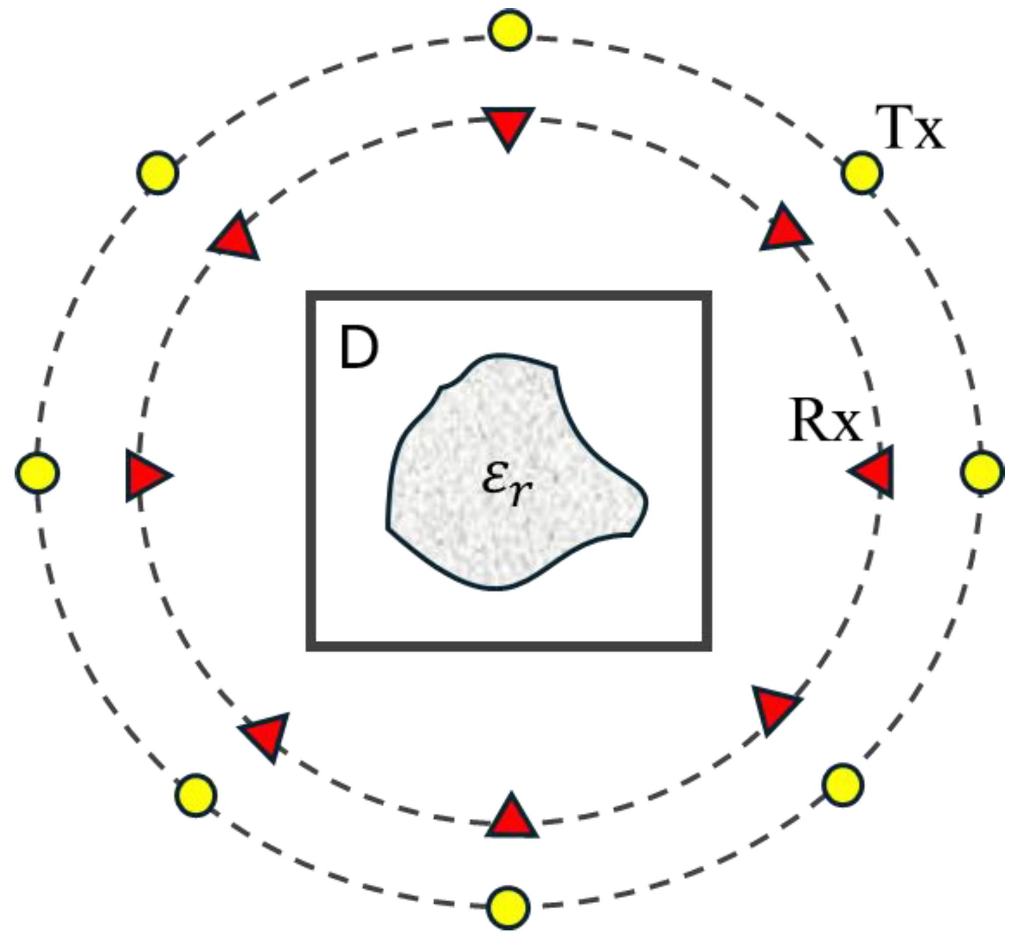
We posit that an unknown object is positioned along the z-axis in free space, as illustrated in Figure 1. ${\stackrel{̿}{\mathsf{\epsilon }}}_{\mathrm{r}}$ denotes the dielectric constant tensor of the object. ${\mathsf{\mu }}_0$ represents the magnetic permeability. The corresponding x-, y-, and z-direction diagonal components of ${\stackrel{̿}{\mathsf{\epsilon }}}_{\mathrm{r}}$ are expressed as ${\mathsf{\epsilon }}_{\mathrm{x}}(\mathrm{x},\mathrm{y})$, ${\mathsf{\epsilon }}_{\mathrm{y}}(\mathrm{x},\mathrm{y})$, and ${\mathsf{\epsilon }}_{\mathrm{z}}\left(\mathrm{x},\mathrm{y}\right)$, respectively. Tx is the transmitter antenna, Rx is the receiver antenna, and D is the domain of interest.

We focus on reconstructing uniaxial objects in free space, assuming a time dependence of $e^{j\omega t}$. We examine two distinct types of incident waves, as detailed below.

• Transverse magnetic waves

In the TM case, the formula for the incident electric field can be expressed as follows:

$${\overline{E}}^i\left(\rho \right)=E_z^i\left(\rho \right)\widehat{z}=e^{-j{k}_0(x\mathit{cos}\mathrm{\varnothing }+y\mathit{sin}\mathrm{\varnothing })}\widehat{z}$$

(1)

Let us consider an incident wave that only has a z component and a scatterer that extends infinitely in the z direction. The total and scattered electric fields can be represented as $\overline{E}=E_z\widehat{z}$ and ${\overline{E}}^s=E_z^s\widehat{z}$, respectively. The respective scalar equations for the scattered electric and total fields can be obtained as follows:

$$E_z\left(\rho \right)={\int }_{s}G\left(\rho ,\rho ’\right)\left({\epsilon }_z\left(\rho ’\right)-1\right)E_z\left(\rho ’\right)d{s}^{’}+E_z^i\left(\rho \right),\rho ,\rho ’\in D$$

(2)

$$E_z^s\left(\rho \right)={\int }_{s}G\left(\rho ,\rho ’\right)\left({\epsilon }_z\left(\rho ’\right)-1\right)E_z\left(\rho ’\right)d{s}^{’},\rho \notin D,\rho ’\in D$$

(3)

The two-dimensional free-space Green’s function is given by the equation $\mathrm{G}\left(\rho ,\rho \mathrm{’}\right)=-{\displaystyle \frac{\mathrm{j}{\mathrm{k}}_0^2}{4}}{\mathrm{H}}_0^{\left(2\right)}\left({\mathrm{k}}_0\left|\rho -\rho \mathrm{’}\right|\right)$, where ${\mathrm{H}}_0^{\left(2\right)}$ denotes the zero-order Hankel function of the second kind. D is the object domain.

2.

Transverse electric waves

In the case of TE waves, the equations given by the $E_x^i\left(\rho \right)$ and $E_y^i\left(\rho \right)$ incident waves are:

$$E_x^i\left(\rho \right)=-\mathit{sin}\varnothing e^{-j{k}_0(x\mathit{cos}\varnothing +y\mathit{sin}\varnothing )}$$

(4)

$$E_y^i\left(\rho \right)=\mathit{cos}\varnothing e^{-j{k}_0(x\mathit{cos}\varnothing +y\mathit{sin}\varnothing )}$$

(5)

$E_x$ and $E_y$ are interdependent. By applying the vector potential technique, the incident field ${\overline{E}}^i\left(\rho \right)=E_x^i\left(\rho \right)\widehat{x}+E_y^i\left(\rho \right)\widehat{y}$ is used to estimate the scattered fields. The external scattered field ${\overline{E}}^s\left(\rho \right)=E_x^s\left(\rho \right)\widehat{x}+E_y^s\left(\rho \right)\widehat{y}$ and the total field $\overline{E}\left(\rho \right)=E_x\left(\rho \right)\widehat{x}+E_y\left(\rho \right)\widehat{y}$ can be expressed by Equations (6)–(9).

$$E_x\left(\rho \right)=\left({\displaystyle \frac{{\partial }^2}{\partial x^2}}+{k_0}^2\right)\left[{\int }_{s}G\left(\rho ,\rho ’\right)\left({\epsilon }_x\left(\rho ’\right)-1\right)E_x\left(\rho ’\right)d{s}^{’}\right]+{\displaystyle \frac{{\partial }^2}{\partial x\partial y}}\left[{\int }_{s}G\left(\rho ,\rho ’\right)\left({\epsilon }_y\left(\rho ’\right)-1\right)E_y\left(\rho ’\right)d{s}^{’}\right]+{\stackrel{⃑}{E}}_x^i\left(\rho \right)$$

(6)

$$E_y\left(\rho \right)={\displaystyle \frac{{\partial }^2}{\partial x\partial y}}\left[{\int }_{s}G\left(\rho ,\rho ’\right)\left({\epsilon }_x\left(\rho ’\right)-1\right)E_x\left(\rho ’\right)d{s}^{’}\right]+\left({\displaystyle \frac{{\partial }^2}{\partial x^2}}+{k_0}^2\right)\left[{\int }_{s}G\left(\rho ,\rho ’\right)\left({\epsilon }_y\left(\rho ’\right)-1\right)E_y\left(\rho ’\right)d{s}^{’}\right]+{\stackrel{⃑}{E}}_y^i\left(\rho \right)$$

(7)

$$E_x^s\left(\rho \right)=\left({\displaystyle \frac{{\partial }^2}{\partial x^2}}+{k_0}^2\right)\left[{\int }_{s}G\left(\rho ,\rho ’\right)\left({\epsilon }_x\left(\rho ’\right)-1\right)E_x\left(\rho ’\right)d{s}^{’}\right]+{\displaystyle \frac{{\partial }^2}{\partial x\partial y}}\left[{\int }_{s}G\left(\rho ,\rho ’\right)\left({\epsilon }_y\left(\rho ’\right)-1\right)E_y\left(\rho ’\right)d{s}^{’}\right]$$

(8)

$$E_y^s\left(\rho \right)={\displaystyle \frac{{\partial }^2}{\partial x\partial y}}\left[{\int }_{s}G\left(\rho ,\rho ’\right)\left({\epsilon }_x\left(\rho ’\right)-1\right)E\widehat{x}\left(\rho ’\right)d{s}^{’}\right]+\left({\displaystyle \frac{{\partial }^2}{\partial x^2}}+{k_0}^2\right)\left[{\int }_{s}G\left(\rho ,\rho ’\right)\left({\epsilon }_y\left(\rho ’\right)-1\right)E\widehat{y}\left(\rho ’\right)d{s}^{’}\right]$$

(9)

In the case of TM for the direct problem, we assume that the distribution of the dielectric constant is known. Equations (1)–(3) can be used to determine both the scattered and total electric fields in the z axis. Likewise, for the TE case, we can employ Equations (4)–(9) to ascertain the scattered fields and total in the x and y axes.

3. Scattered Field Generative Adversarial Networks

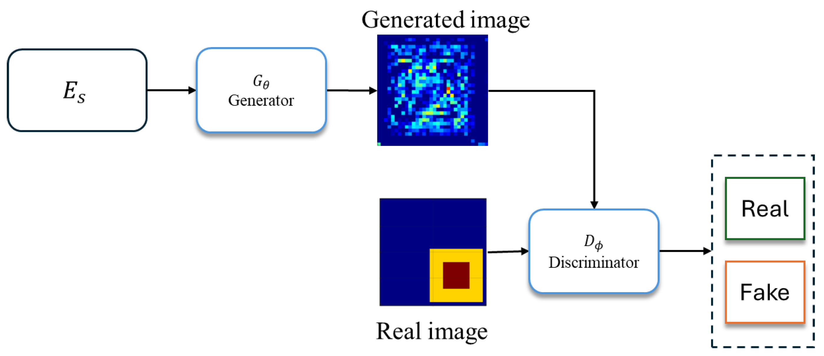
The GANs are made up of a generator and a discriminator that are trained in a mutually resisting manner. This model has shown remarkable success in various applications, such as style migration, image generation, and image-to-image translation. Despite their success, training GANs poses significant challenges caused by vanishing gradients as well as instability. To overcome these challenges, researchers have proposed various GAN models with improved stability and scalability to address a wider range of applications. The GANs illustrated in Figure 2 designate the generator as $G_{\theta }$ and the discriminator as $D_{\mathrm{\varnothing }}$. Here, θ and ∅ are used to symbolize the unknown parameters of the generator and discriminator, respectively. In this paper, we feed measured scattered fields into the training model. 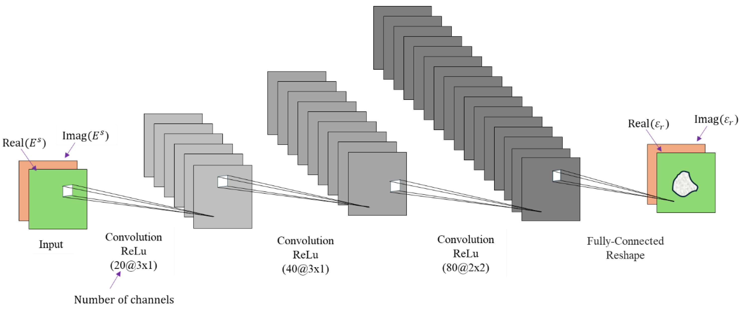Then, the generator ($G_{\theta }$) repeatedly generates images for the discriminator ($D_{\mathrm{\varnothing }}$) to determine the authenticity of the image (i.e., real and fake). Through this process, each neural parameter is trained, and accurate electromagnetic image reconstruction is achieved. We use a DRCNN (deep residual convolutional neural network) as the generation network for the SF-GANs. This network is designed to process and analyze complex, dispersed field information. The architecture of the DRCNN includes three convolutional layers, each of which is followed by a ReLu activation function. 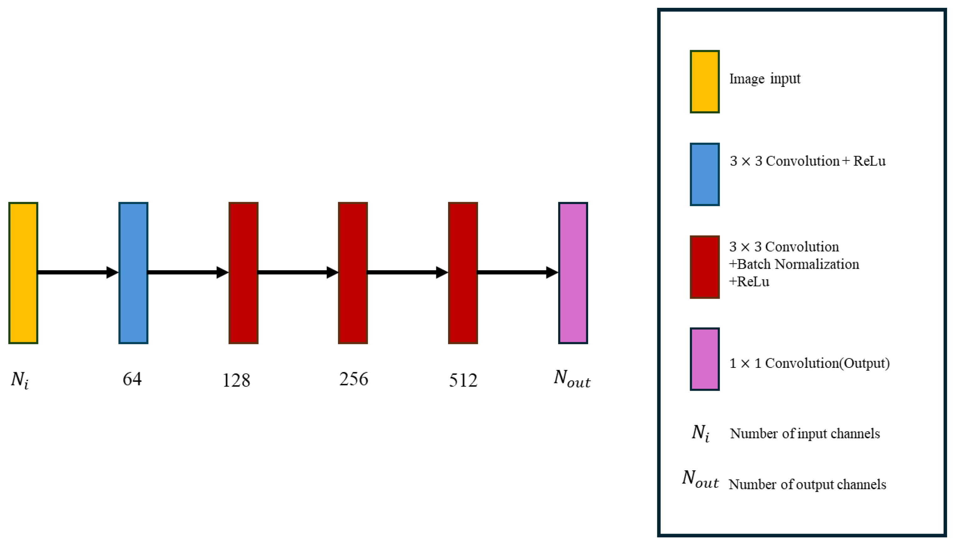Figure 3 shows the architecture of the GAN generator. The final step in the process involves accurately reconstructing the dielectric constant distribution using fully connected and reshaped layers. The architecture of the discriminator consists of repeatedly adding convolutional layers, batch normalization layers, and ReLu layers, as depicted in Figure 4. The discriminator analyzes the image generated by the generator and provides a score, thereby determining whether the generator should adjust its training weights. This iterative procedure persists until an optimal equilibrium is established.

The generator’s loss function, $L_{GAN}^G$, is expressed as follows:

$$L_{GAN}^G\left(\theta |\varnothing \right)=L_{RMSE}\left(\theta \right)+\gamma L_A\left(\theta |\varnothing \right)$$

(10)

In this context, $L_{RMSE}\left(\theta \right)$ quantifies the discrepancy between the restored image and the ground truth image. $\gamma$ is the weight of $L_A$ in the generator loss function. The root mean square error (RMSE) is defined by the following formula:

$$L_{RMSE}={\displaystyle \frac{1}{M}}\sum _{i=1}^M{\displaystyle \frac{{‖{\stackrel{̿}{\epsilon }}_r-{\stackrel{̿}{\epsilon }}_r^r‖}_F}{{‖{\stackrel{̿}{\epsilon }}_r‖}_F}}$$

(11)

Here, ${\stackrel{̿}{\epsilon }}_r$ and ${\stackrel{̿}{\epsilon }}_r^r$ denote the true and restored permittivity, respectively. F symbolizes the Frobenius norm, and M represents the number of tests conducted.

$$L_A\left(\theta |\varnothing \right)={\displaystyle \frac{1}{N}}\sum _{i=1}^N{‖D_{\varnothing }\left(G_{\theta }\left(X_i\right)\right)-1‖}_1$$

(12)

$L_A$ acts as the scoring mechanism for the discriminator, evaluating the accuracy of the entire reconstructed image. $N$ denotes the batch number, and $X_i$ denotes the trained data.

The discriminator’s loss function can be formulated as follows:

$$L_{GAN}^D\left(\theta |\varnothing \right)={\displaystyle \frac{1}{2N}}\sum _{i=1}^N\left({‖D_{\varnothing }\left(Y_i\right)-1‖}_2^2+{‖D_{\varnothing }\left(G_{\theta }\left(X_i\right)\right)‖}_2^2\right)$$

(13)

In this context, $\mathrm{\varnothing }$ represents the unknown parametric data, while $\theta$ is the weight parameter. $Y_i$ refers to the true data. The optimization process alternates between focusing on $D_{\mathrm{\varnothing }}$ and $G_{\theta }$ in an adversarial manner until a Nash equilibrium is achieved. Essentially, the process continues until the generator $G_{\theta }\left(X\right)$ produces a closely resembling image, making it indistinguishable from the authentic data by the discriminator $D_{\mathrm{\varnothing }}$.

4. Numerical Results

In our study, we place a two-dimensional uniaxial object in free space with transmitters and receivers positioned evenly around the object. We emit TM waves and TE waves from various directions to illuminate the object and collect the scattered field. The collected data are then input into the SF-GANs for training, with the aim of eventually generating precise electromagnetic images.

4.1. Configuration of the Scattering System

In our research, we divide the edge of the scatterer into segments of a constant size equal to ${\displaystyle \frac{0.2{\lambda }_0}{\sqrt{{\epsilon }_r}}}$. ${\lambda }_0$ and ${\epsilon }_r$ represent the wavelength in free space and the relative dielectric constant of the uniaxial object, respectively. The scatterer’s dielectric coefficient varies from 1 to 8, and the frequency of the incident wave is set at 3 GHz. For the simulation, we set up a uniform configuration of 32 transmitting and 32 receiving antennas. To mimic real-world conditions, we add 5% and 20% noise in our simulation.

4.2. Training Detail

During the training, we use the scattered field as input for the SF-GANs to allow the neural network to emulate Maxwell’s equations and generate electromagnetic imaging. In the realm of artificial intelligence (AI), the 80–20 principle is applied to the training and testing sets. We then use an adaptive moment estimation (ADAM) optimizer to train the neural network, with a learning rate of 0.0002, a maximum epoch of 200, and a mini-batch size of 32.

We use Equation (14) below to measure the performance of each scenario.

$$RMSE={\displaystyle \frac{1}{M_t}}{\displaystyle \frac{{\sum _{i=1}^{M_t}‖{\stackrel{̿}{\epsilon }}_r-{\stackrel{̿}{\epsilon }}_r^r‖}_F}{{‖{\stackrel{̿}{\epsilon }}_r‖}_F}}$$

(14)

${\stackrel{̿}{\epsilon }}_r$ is the true permittivity, while ${\stackrel{̿}{\epsilon }}_r^r$ is the reconstructed relative permittivity. $M_t$ denotes the number of tests conducted. F represents the Frobenius norm. The structural similarity index measure (SSIM) is then defined to compare the simulated results for different cases.

$$SSIM={\displaystyle \frac{\left(2{\mu }_{\tilde{y}}{\mu }_y+C_1\right)\left(2{\sigma }_{\tilde{y}y}+C_2\right)}{\left({\mu }_{\tilde{y}}^2+{\mu }_y^2+C_1\right)\left({\sigma }_{\tilde{y}}^2+{\sigma }_y^2+C_2\right)}},$$

(15)

Here, y and $\tilde{y}$ denote the true and reconstructed relative permittivity profiles, respectively. ${\mathsf{\mu }}_{\mathrm{y}}$ represents the mean of y. ${\sigma }_{\tilde{y}}^2$ and ${\sigma }_{\tilde{y}y}$ are the variance of y and the covariance of $\tilde{y}$ and y, respectively. Two small constraints, $C_1={\left({\mathrm{K}}_1\mathrm{D}\right)}^2$ and $C_2={\left({\mathrm{K}}_2\mathrm{D}\right)}^2$, are added to prevent a zero denominator, with ${\mathrm{K}}_1=0.01$ and ${\mathrm{K}}_2=0.03$ as the two hyperparameters. $\mathrm{D}$ is the dynamic range of pixels for image y.

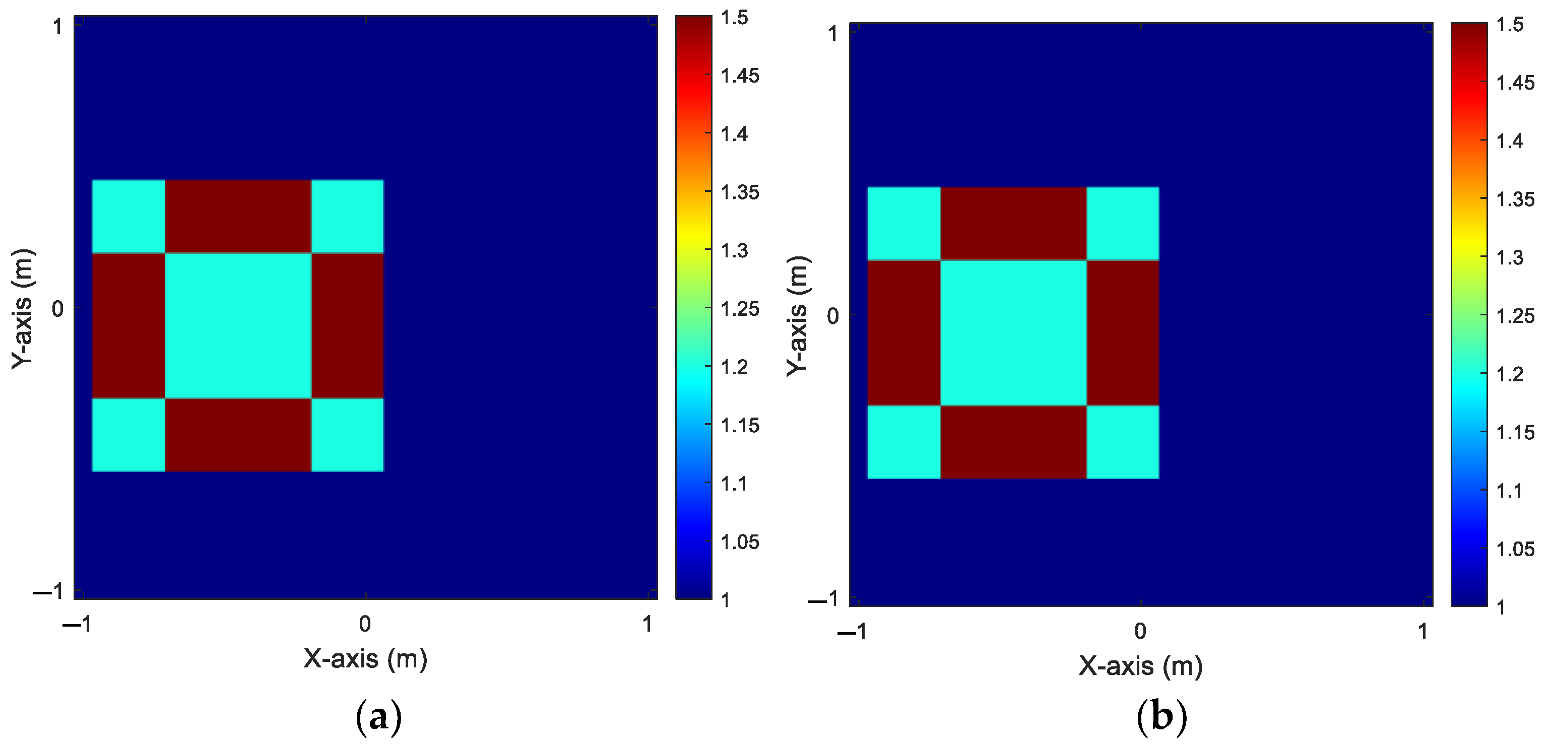
4.3. Relative Permittivity from 1 to 1.5

In this simulation, we focus on establishing a distribution of dielectric constants ranging from 1 to 1.5. Our analysis involved 10 scatterers, each characterized by a unique dielectric constant distribution. These scatterers are positioned within the measurement area, with the flexibility to move to 50 different locations. To simulate real-world conditions, we introduce 20% noise into the environment. Using the scattered field data, we employ SF-GANs to iteratively train and reconstruct accurate electromagnetic images. 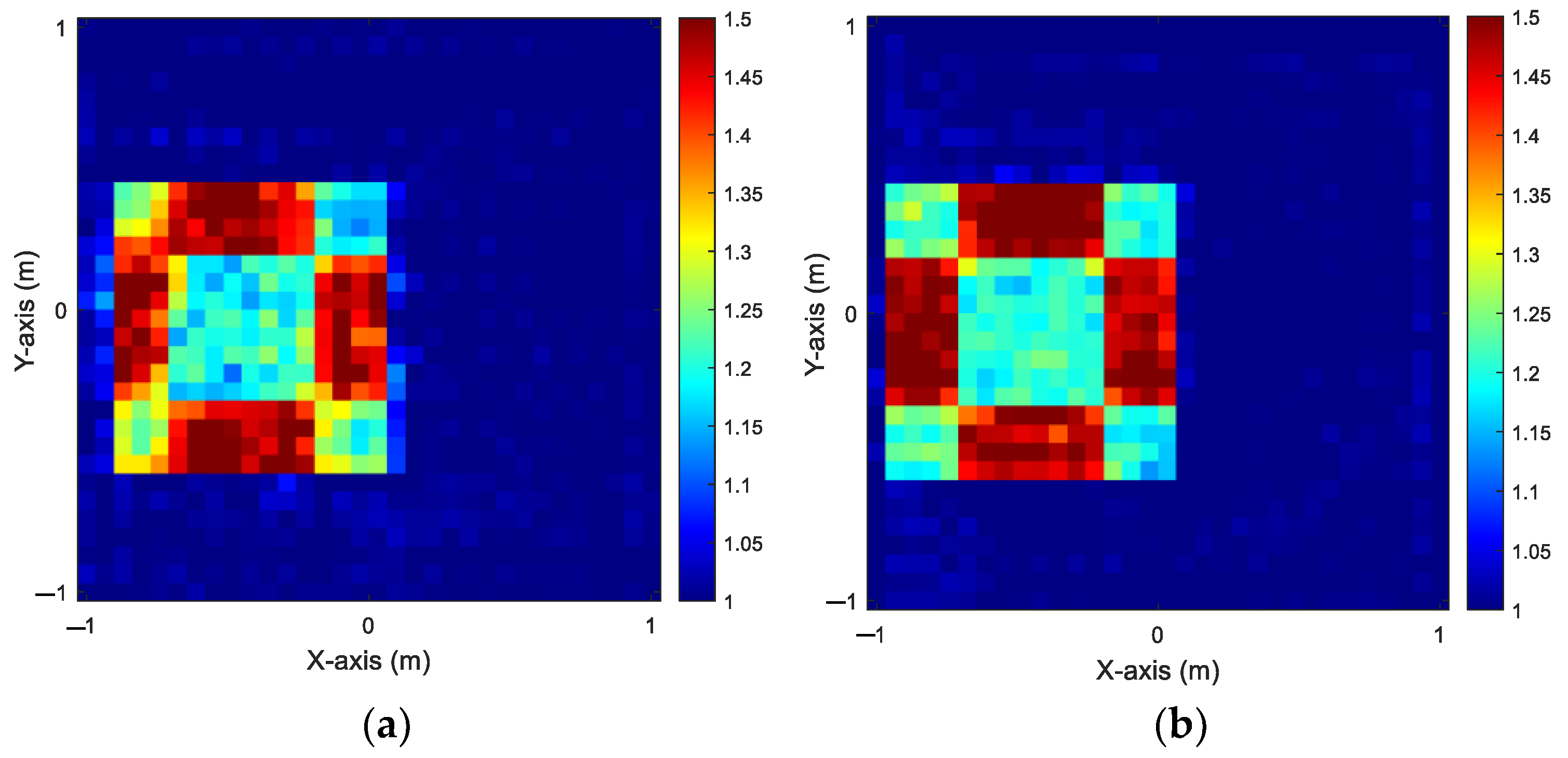The ground truth of ${\epsilon }_z$ and ${\epsilon }_x$ for relative permittivity ranges from 1 to 1.5 can be found in Figure 5. The reconstructed results of ${\epsilon }_z$ and ${\epsilon }_x$ by BP-GANs and SF-GANs can be found in Figure 6 and Figure 7, respectively.

Table 2. Reconstructed performance of case 4.3 with 20% noise.

Performance		${\mathit{\epsilon }}_{\mathit{z}}$	${\mathit{\epsilon }}_{\mathit{x}}$
BP-GANs	RMSE SSIM	3.43%	1.66%
		93.41%	97.8%
SF-GANs	RMSE SSIM	0.63%	0.65%
		99.32%	99.03%

offers an overview of the performance metrics related to the reconstruction process. When comparing BP-GANs to SF-GANs under the same noise, it is evident that the image quality of GANs with backpropagation is notably inferior in terms of clarity and sharpness.

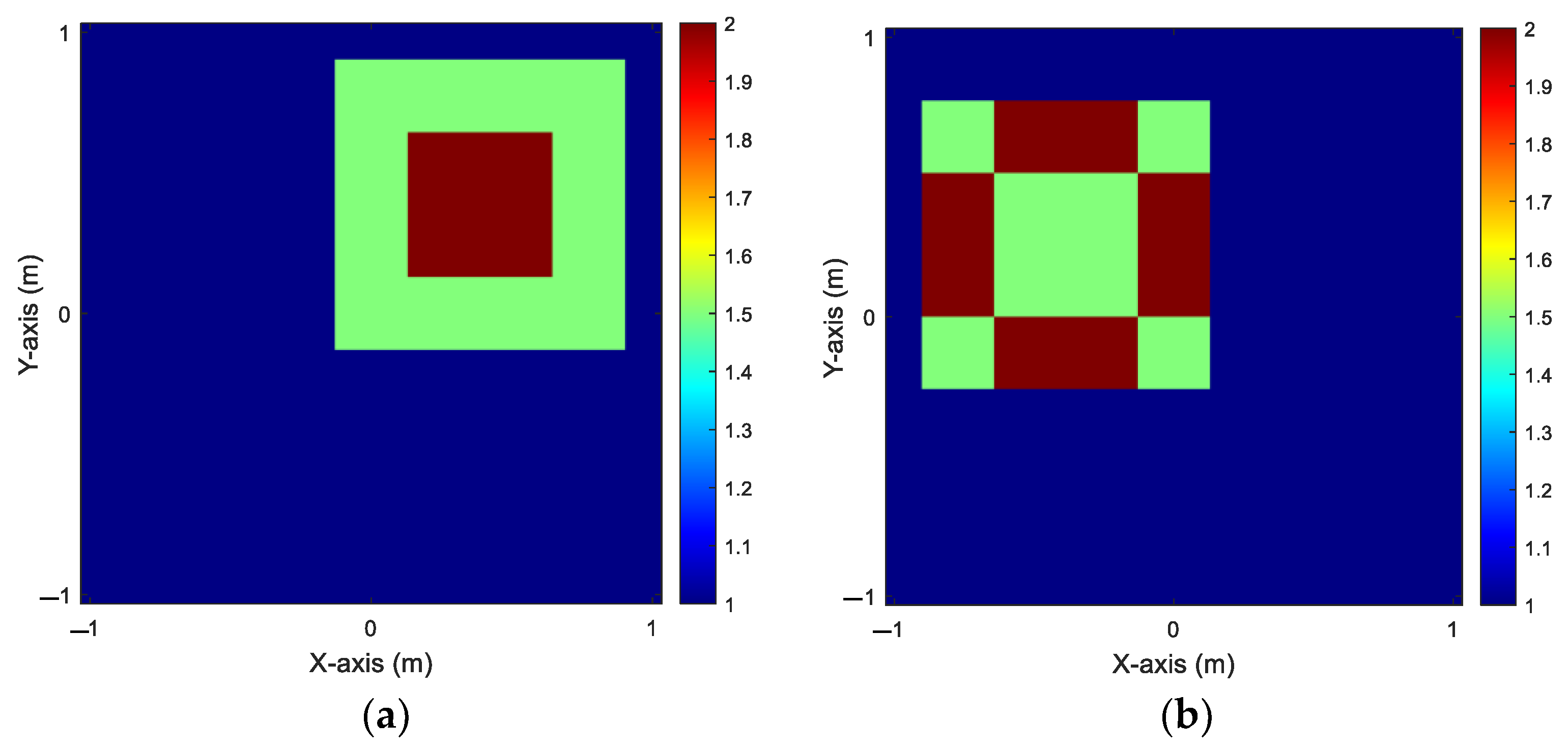
4.4. Relative Permittivity from 1.5 to 2

In this simulation, we focus on finding the range of dielectric constants from 1.5 to 2. Ten scatterers with unique dielectric constant distributions are studied. The scatterers are positioned at up to 50 different locations for measurement. To mimic real-world conditions, 5% noise is added. We apply SF-GANs to train the collected scattered fields and create accurate electromagnetic images. 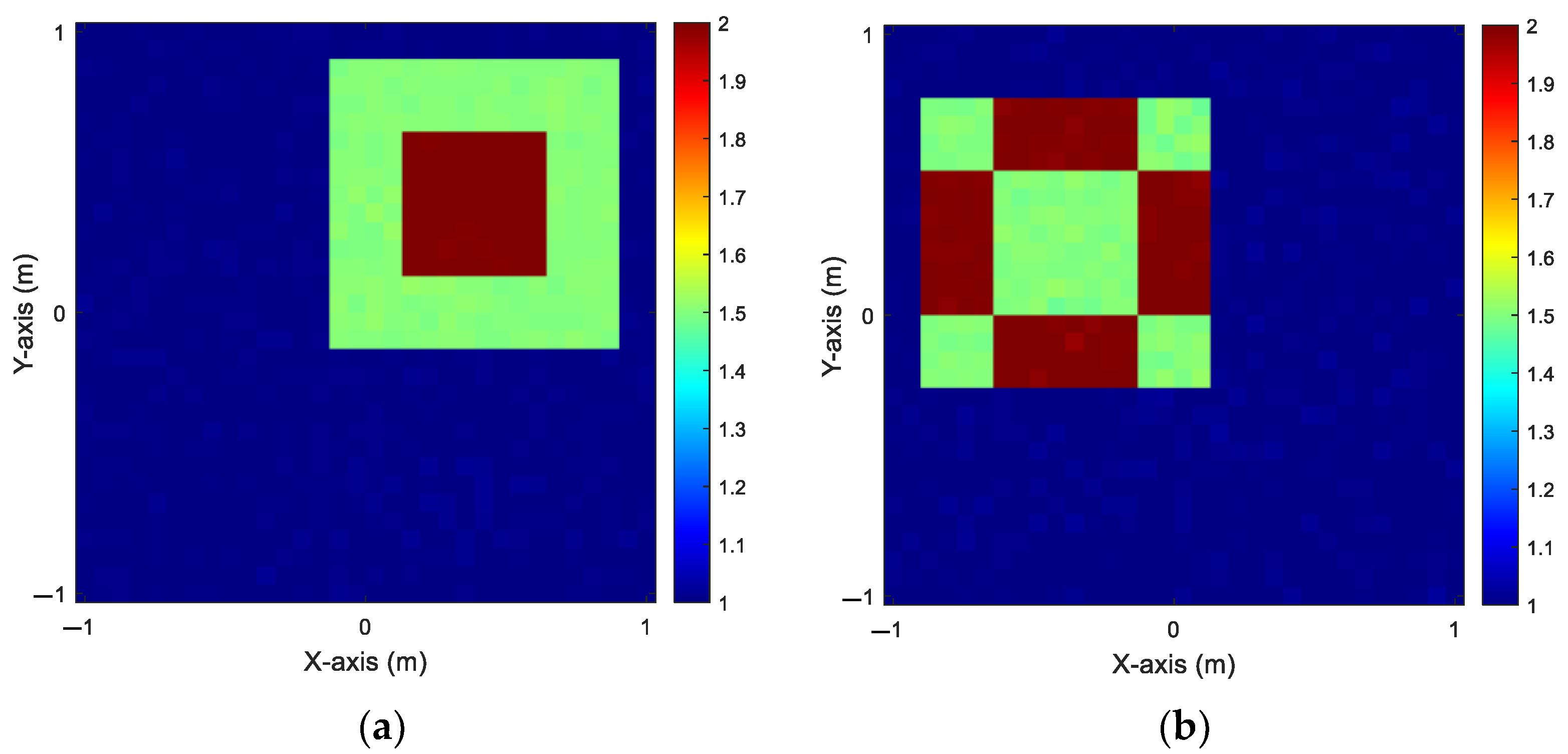The accurate permittivity values for ${\epsilon }_z$ and ${\epsilon }_x$ ranging from 1.5 to 2 are shown in Figure 8. The reconstructed results for ${\epsilon }_z$ and ${\epsilon }_x$ using BP-GANs and SF-GANs can be found in Figure 9 and Figure 10, respectively.

Table 3. Reconstructed performance of case 4.4 with 5% noise.

Performance		${\mathit{\epsilon }}_{\mathit{z}}$	${\mathit{\epsilon }}_{\mathit{x}}$
BP-GANs	RMSE SSIM	2.43%	2.19%
		98.75%	99.03%
SF-GANs	RMSE SSIM	0.76%	0.85%
		98.51%	98.95%

provides an overview of the performance metrics for the reconstruction process.

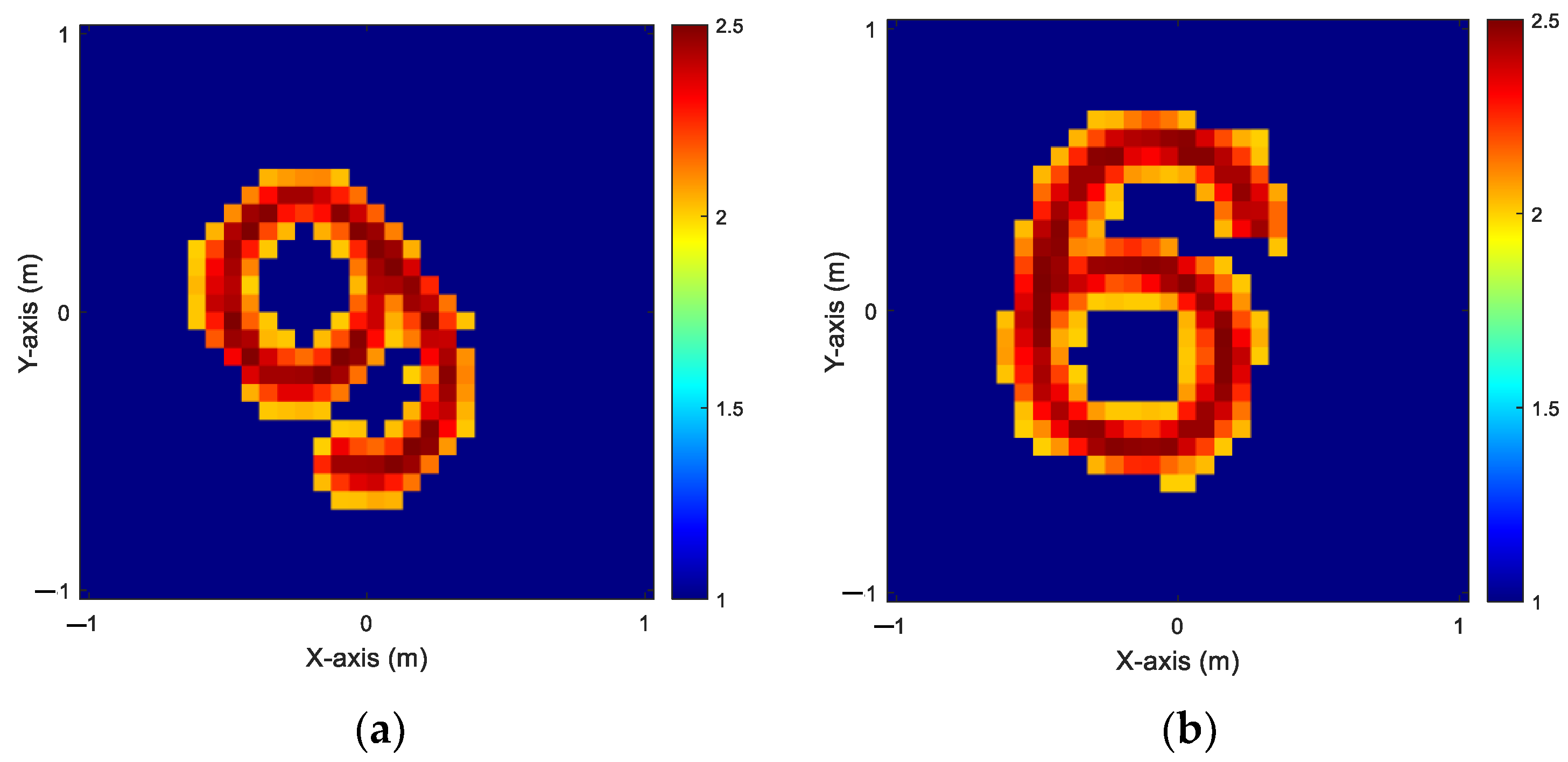
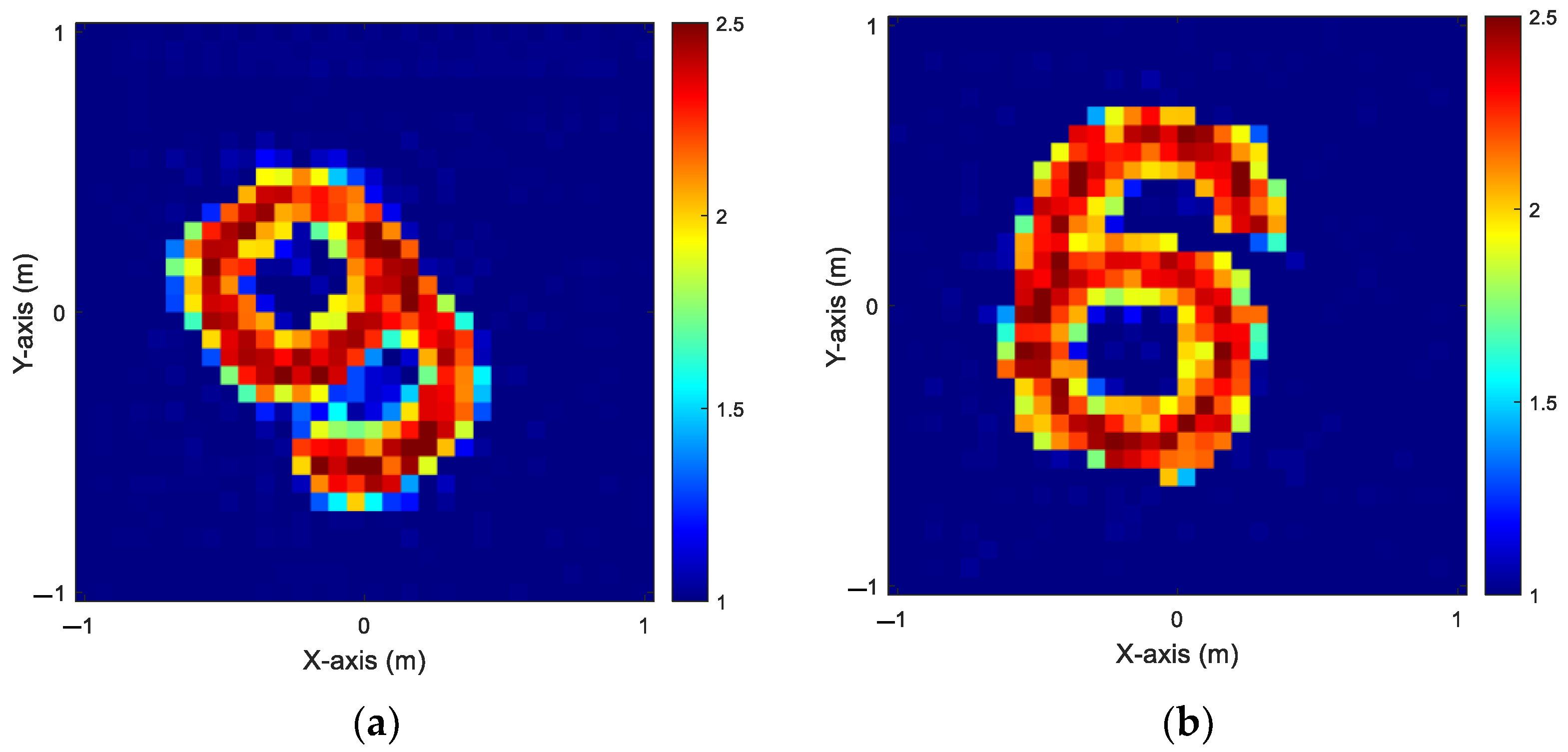
4.5. MNIST from 2 to 2.5

The Modified National Institute of Standards and Technology (MNIST) database contains a large set of handwritten digits that is commonly used for training various image processing systems. The MNIST database has 60,000 training images and 10,000 testing images, each measuring 28 × 28 pixels. The dataset is organized so that every 50 consecutive images represent a different style of handwriting, each shown at 50 different angles. The MNIST database is widely used to train neural network architectures for image processing due to its simplicity. In this case, we simulate an environment with 32 transmitters and 32 receivers and distribute the dielectric coefficient from 2 to 2.5. We add 5% noise to each transmitter–receiver pair. To create a dataset for training, we randomly select 50 images of each handwritten digit (0–9) from the MNIST dataset, resulting in a total of 500 images for each case. This dataset is then split into two subsets—80% for training and 20% for testing—to speed up the process. The relative permittivity for ${\epsilon }_z$ and ${\epsilon }_x$ ranging from 2 to 2.5 is shown in Figure 11. The reconstructed results for ${\epsilon }_z$ and ${\epsilon }_x$ using BP-GANs and SF-GANs are shown in Figure 12 and Figure 13, respectively.

Table 4. Reconstructed performance of case 4.5 with 5% noise.

Performance		${\mathit{\epsilon }}_{\mathit{z}}$	${\mathit{\epsilon }}_{\mathit{x}}$
BP-GANs	RMSE SSIM	5.96%	5.21%
		95.13%	95.39%
SF-GANs	RMSE SSIM	1.96%	3.96%
		95.43%	96.04%

provides an overview of the performance metrics for the reconstruction process.

Nonlinear phenomena in electromagnetic imaging have long been an unsolved challenge that has garnered significant attention. Unlike the TM case, the TE case is influenced by both x and y components, making the nonlinear situation more intricate and leading to a substantial impact on image resolution. Our numerical findings indicate that our proposed method can effectively address the nonlinear problem in electromagnetic imaging. In this research, though we do observe that the nonlinearity will become significant as the dielectric coefficient distribution grows larger, satisfactory reconstruction results may still be achieved. In our simulation, we utilized a personal computer equipped with a 3.4 GHz Intel Core i7 processor, 64 GB of RAM, and an NVIDIA GeForce RTX 40 series GPU. Training the SF-GANs on this setup takes approximately 26 min, while testing with the proposed SF-GANs takes less than one second.

5. Conclusions

We propose SF-GANs to solve ISPs for uniaxial objects in this research. Because the dielectric constant components will propagate in different directions, the nonlinear phenomenon of TE waves will be more pronounced than that of TM waves. This makes the reconstruction using the scattered fields challenging. Numerical simulations and experimental results show that SF-GANs have overwhelming advantages in reconstructing uniaxial objects. Our investigation concludes that the proposed SF-GANs architecture eligibly handles complex TE scenarios and successfully overcomes the diverse challenges encountered in ISPs. In the future, we plan to focus on integrating attention-based neural network architectures into the SF-GAN framework and implementing them in more intricate situations, such as the reconstruction of buried objects in half-space. Furthermore, we will also explore the possibility of combining the SF-GAN architecture with the switch transformer model to further enhance the quality of reconstructed images.

References

- Uecker, M.; Hohage, T.; Block, K.T.; Frahm, J. Image reconstruction by regularized nonlinear inversion-joint estimation of coil sensitivities and image content. Magn. Reson. Med. 2008, 60, 674–682. [Google Scholar] [CrossRef] [PubMed]
- Deisboeck, T.; Kresh, J.Y. Complex Systems Science in Biomedicine; Springer Science & Business Media: New York, NY, USA, 2007. [Google Scholar]
- Song, L.-P.; Yu, C.; Liu, Q.H. Through-wall imaging (TWI) by radar: 2-D tomographic results and analyses. IEEE Trans. Geosci. Remote Sens. 2005, 43, 2793–2798. [Google Scholar] [CrossRef]
- Chen, X.; Wei, Z.; Li, M.; Rocca, P. A review of deep learning approaches for inverse scattering problems. Prog. Electromagn. Res. 2020, 167, 67–81. [Google Scholar] [CrossRef]
- Sanghvi, Y.; Kalepu, Y.; Khankhoje, U.K. Embedding deep learning in inverse scattering problems. IEEE Trans. Comput. Imaging 2019, 6, 46–56. [Google Scholar] [CrossRef]
- Habashy, T.M.; Groom, R.W.; Spies, B.R. Beyond the Born and Rytov approximations: A nonlinear approach to electromagnetic scattering. J. Geophys. Res. Solid Earth 1993, 98, 1759–1775. [Google Scholar] [CrossRef]
- Belkebir, K.; Chaumet, P.C.; Sentenac, A. Super resolution in total internal reflection tomography. J. Opt. Soc. Am. A 2005, 22, 1889–1897. [Google Scholar] [CrossRef]
- Chen, X. Computational Methods for Electromagnetic Inverse Scattering; Wiley-IEEE Press: New York, NY, USA, 2018. [Google Scholar]
- Chew, W.C.; Wang, Y.-M. Reconstruction of two-dimensional permittivity distribution using the distorted Born iterative method. IEEE Trans. Med. Imaging 1990, 9, 218–225. [Google Scholar] [CrossRef]
- Van den Berg, P.M.; Kleinman, R.E. A contrast source inversion method. Inverse Probl. 1997, 13, 1607. [Google Scholar] [CrossRef]
- Chen, X. Subspace-based optimization method for solving inverse scattering problems. IEEE Trans. Geosci. Remote Sens. 2010, 48, 42–49. [Google Scholar] [CrossRef]
- Krizhevsky, A.; Sutskever, I.; Hinton, G.E. Imagenet classification with deep convolutional neural networks. Proc. Adv. Neural Inf. Process. Syst. 2012, 25, 1097–1105. [Google Scholar] [CrossRef]
- Simonyan, K.; Zisserman, A. Very deep convolutional networks for large-scale image recognition. arXiv 2014. [Google Scholar] [CrossRef]
- Du, J.; Xu, Y. Hierarchical deep neural network for multivariate regression. Pattern Recognit. 2017, 63, 149–157. [Google Scholar] [CrossRef]
- Guo, R.; Jia, Z.; Song, X.; Li, M.; Yang, F.; Xu, S.; Abubakar, A. Pixel-and model-based microwave inversion with supervised descent method for dielectric targets. IEEE Trans. Antennas Propag. 2020, 68, 8114–8126. [Google Scholar] [CrossRef]
- Song, T.; Kuang, L.; Han, L.; Wang, Y.; Liu, Q.H. Inversion of rough surface parameters from SAR images using simulation-trained convolutional neural networks. IEEE Geosci. Remote Sens. Lett. 2018, 15, 1130–1134. [Google Scholar] [CrossRef]
- Huang, Y.; Song, R.; Xu, K.; Ye, X.; Li, C.; Chen, X. Deep Learning-Based Inverse Scattering with Structural Similarity Loss Functions. IEEE Sens. J. 2021, 21, 4900–4907. [Google Scholar] [CrossRef]
- Guo, L.; Song, G.; Wu, H. Complex-Valued Pix2pix—Deep Neural Network for Nonlinear Electromagnetic Inverse Scattering. Electronics 2021, 10, 752. [Google Scholar] [CrossRef]
- Xu, K.; Zhang, C.; Ye, X.; Song, R. Fast Full-Wave Electromagnetic Inverse Scattering Based on Scalable Cascaded Convolutional Neural Networks. IEEE Trans. Geosci. Remote Sens. 2022, 60, 1–11. [Google Scholar] [CrossRef]
- Xu, K.; Qian, Z.; Zhong, Y.; Su, J.; Gao, H.; Li, W. Learning-Assisted Inversion for Solving Nonlinear Inverse Scattering Problem. IEEE Trans. Microw. Theory Tech. 2023, 71, 2384–2395. [Google Scholar] [CrossRef]
- Wu, Z.; Peng, Y.; Wang, P.; Wang, W.; Xiang, W. A Physics-Induced Deep Learning Scheme for Electromagnetic Inverse Scattering. IEEE Trans. Microw. Theory Tech. 2024, 72, 927–947. [Google Scholar] [CrossRef]
- Yao, H.M.; Jiang, L.; Ng, M. Enhanced Deep Learning Approach Based on the Conditional Generative Adversarial Network for Electromagnetic Inverse Scattering Problems. IEEE Trans. Antennas Propag. 2024, 72, 6133–6138. [Google Scholar] [CrossRef]
- Wang, Y.M.; Chew, W.C. An iterative solution of the two-dimensional electromagnetic inverse scattering problem. Int. J. Imaging Syst. Technol. 1989, 1, 100–108. [Google Scholar] [CrossRef]
- Pastorino, M.; Massa, A.; Caorsi, S. A microwave inverse scattering technique for image reconstruction based on a genetic algorithm. IEEE Trans. Instrum. Meas. 2000, 49, 573–578. [Google Scholar] [CrossRef]
- Agarwal, K.; Chen, X. Application of Differential Evolution in 2- Dimensional Electromagnetic Inverse Problems. In Proceedings of the IEEE Congress on Evolutionary Computation, Singapore, 25–28 September 2007; pp. 4305–4312. [Google Scholar]
- Pastorino, M. Stochastic optimization methods applied to microwave imaging: A review. IEEE Trans. Antennas Propag. 2007, 55, 538–548. [Google Scholar] [CrossRef]
- Ran, P.; Qin, Y.; Lesselier, D. Electromagnetic imaging of a dielectric micro-structure via convolutional neural networks. In Proceedings of the IEEE 2019 27th European Signal Processing Conference (EUSIPCO), Coruña, Spain, 1–5 September 2019. [Google Scholar]
- Fajardo, J.E.; Galván, J.; Vericat, F.; Carlevaro, C.M.; Irastorza, R.M. Phaseless microwave imaging of dielectric cylinders: An artificial neural networks-based approach. Prog. Electromagn. Res. 2019, 166, 95–105. [Google Scholar] [CrossRef]
- Wei, Z.; Chen, X. Deep-learning schemes for full-wave nonlinear inverse scattering problems. IEEE Trans. Geosci. Remote Sens. 2019, 57, 1849–1860. [Google Scholar] [CrossRef]
- Yao, H.M.; Wei, E.I.; Jiang, L. Two-step enhanced deep learning approach for electromagnetic inverse scattering problems. IEEE Antennas Wirel. Propag. Lett. 2019, 18, 2254–2258. [Google Scholar] [CrossRef]
- Guo, R.; Song, X.; Li, M.; Yang, F.; Xu, S.; Abubakar, A. Supervised descent learning technique for 2-D microwave imaging. IEEE Trans. Antennas Propag. 2019, 67, 3550–3554. [Google Scholar] [CrossRef]
- Chen, G.; Shah, P.; Stang, J.; Moghaddam, M. Learning-assisted multi-modality dielectric imaging. IEEE Trans. Antennas Propag. 2019, 68, 2356–2369. [Google Scholar] [CrossRef]
- Sun, Y.; Xia, Z.; Kamilov, U.S. Efficient and accurate inversion of multiple scattering with deep learning. Opt. Express 2018, 26, 14678–14688. [Google Scholar] [CrossRef]
- Li, L.; Wang, L.G.; Teixeira, F.L.; Liu, C.; Nehorai, A.; Cui, T.J. DeepNIS: Deep neural network for nonlinear electromagnetic inverse scattering. IEEE Trans. Antennas Propag. 2019, 67, 1819–1825. [Google Scholar] [CrossRef]
- Li, L.; Wang, L.G.; Teixeira, F.L. Performance analysis and dynamic evolution of deep convolutional neural network for electromagnetic inverse scattering. IEEE Antennas Wirel. Propag. Lett. 2019, 18, 2259–2263. [Google Scholar] [CrossRef]
- Xiao, J.; Li, J.; Chen, Y.; Han, F.; Liu, Q.H. Fast electromagnetic inversion of inhomogeneous scatterers embedded in layered media by born approximation and 3-D U-Net. IEEE Geosci. Remote Sens. Lett. 2019, 17, 1677–1681. [Google Scholar] [CrossRef]
- Khoshdel, V.; Ashraf, A.; LoVetri, J. Enhancement of multimodal microwave-ultrasound breast imaging using a deep-learning technique. Sensors 2019, 19, 4050. [Google Scholar] [CrossRef] [PubMed]
- Khoo, Y.; Ying, L. SwitchNet: A neural network model for forward and inverse scattering problems. SIAM J. Sci. Comput. 2019, 41, A3182–A3201. [Google Scholar] [CrossRef]